Article

The Spatial Optimization and Evaluation of the Economic, Ecological, and Social Value of Urban Green Space in Shenzhen

1
Key Laboratory of Urban Land Resources Monitoring and Simulation, MNR, Shenzhen 518034, China
2
Shenzhen Urban Planning and Land Resource Research Center, Shenzhen 518034, China
3
College of Resources and Environment, Huazhong Agricultural University, Wuhan 430070, China
4
School of Information Systems, Singapore Management University, Singapore 178902, Singapore
*
Authors to whom correspondence should be addressed.
Sustainability 2020, 12(5), 1844; https://doi.org/10.3390/su12051844
Submission received: 25 January 2020 / Revised: 20 February 2020 / Accepted: 26 February 2020 / Published: 1 March 2020

Abstract

:
Urban green space (UGS) is important in urban systems, as it benefits economic development, ecological conservation, and living conditions. Many studies have evaluated the economic, ecological, and social value of UGS worldwide, and spatial optimization for UGS has been carried out to maximize its value. However, few studies have simultaneously examined these three values of UGS in one optimization system. To fill this gap, this study evaluated the economic value of UGS in terms of promoting housing prices, its ecological value through the relief of high land surface temperature (LST), and its social value through the provision of recreation spaces for residents within a 255 m distance. Subsequently, these three values were set as objectives in a genetic algorithm (GA)-based multi-objective optimization (MOP) system. Shenzhen was taken as the case study area. The results showed that the influencing distance of UGS in Shenzhen for house prices was 345 m, and the influencing distance of UGS for LST was 135 m. Using MOP, the Pareto solutions for increasing UGS were identified and presented. The results indicate that MOP can simultaneously optimize UGS’s economic, ecological, and social value.

1. Introduction

Urban residents are expected to constitute two-thirds of the world’s population by the year 2050. This is a significant increase from the current figure, as more than half of the global population now lives in cities [1]. Within this context, it is of key importance to provide urban residents with favorable living conditions. Urban green space (UGS) is an essential part of urban systems [2] and offers a diversity of social, economic, and ecological benefits to urban residents [3,4,5].
A large body of literature has shown that UGS has high social value, as it improves urban residents’ quality of life [6,7]. It has a beneficial impact on the physical and mental health of human beings by providing spaces for leisure and physical activity [3,5,8,9,10]. Moreover, UGS can facilitate social cohesion, interaction, and democracy, and may reduce crime rates [11], thereby enhancing urban residents’ quality of life [12].
In addition to its profound social value, UGS also provides significant value for urban residents [13,14]. A large body of literature has shown that UGS can considerably mitigate urban problems [15] through actions such as regulating urban climates, alleviating urban heat island (UHI) effects [16,17], absorbing particle air pollutants, improving air quality, infiltrating storms [18,19,20], reducing noise levels [13], and sequestering carbon [21].
The social and ecological value of UGS is widely accepted, while its economic value is not as immediately recognizable, because the services it provides are public goods without market prices [22]. However, real estate markets in developed countries and regions with good environmental quality indicate that many people are willing to pay more for urban properties that are close to UGS [23,24]. Many studies have estimated the economic value or amenity benefits of urban parks and public open spaces [22,25,26].
In summary, UGS has high social, ecological, and economic value. A comparative plan for UGS is essential for increasing the ecological and socioeconomic benefits of urban development [27]. To date, many studies have examined the spatial optimization of UGS to maximize its value. Huang et al. [27] used a space optimization strategy to improve the quality and accessibility of green spaces and proposed that this optimization method should be used in UGS planning and management. Zhang et al. [28] developed a multi-objective model to evaluate the diurnal cooling of UGS and identify the best locations and configurations for new UGSs. Unal and Uslu [29] attempted to minimize the distances between people and UGS service areas to optimize UGS. Yoon [30] used a multi-objective model to maximize the cooling effect and connectivity of UGS.
Even though the spatial optimization of UGS has often been considered in urban planning research, existing studies typically consider only one function of UGS in their spatial optimization processes, such as its social function (through maximizing accessibility) or ecological function (through maximizing cooling or UHI relief). Few studies have considered the full value of UGS in social, economic, and ecological terms simultaneously in the optimization process. To fill this gap, this study evaluates the social, economic, and ecological value of UGS in Shenzhen and uses the most popular genetic algorithm (GA)-based multi-objective optimization (MOP) model to optimize the spatial distribution of UGS, to simultaneously maximize its social, economic, and ecological value. The GA-based MOP method can seek a set of Pareto solutions for multi-objective problems [31] and has been widely used in land-use optimization [32,33]. Pareto solutions imply that an improvement in one objective must be achieved at the expense of at least one of the other objectives [34,35,36]. Pareto solutions do not provide “one” best solution but a set of non-dominated solutions that can reflect tradeoffs between multiple objectives. The MOP method is popular in the field of land-use optimization, since the traditional linear programming method cannot handle more than one objective. Moreover, the heuristic method GA can address nonlinear and unstructured issues in spatial problems. Therefore, GA-based MOP is used to carry out the optimization for UGS to simultaneously maximize its economic, social, and ecological value. Meanwhile, the widely used hedonic price models [37] are used to evaluate the economic value of UGS-based housing rental prices. The ecological value of UGS is assessed by its relief on UHI in urban areas. Finally, its social value is presented by its accessibility for residents. Shenzhen is chosen as the case study area because of its rapid urbanization and the importance of UGS in its urban system. The UGS considered in this study comprises urban parks and green vegetation, including urban parks, wetlands, grasslands, and forests. According to existing studies, green spaces can be categorized into private green spaces and public green spaces, based on ownership [38]. In this study, only the public UGS is considered. The remainder of this paper is organized as follows. The second section introduces the study area and data sources; the third section details the methods used in this study; and the fourth and fifth sections present the results, conclusions, and discussion.

2. Study Area and Data Sources

2.1. Study Area

Shenzhen (22°27′ N to 22°52′ N, 113°46′ N to 114°37′ N) is a coastal city in southern China, located in the Pearl River Delta Region (Figure 1). The city forms a passageway from mainland China to Hong Kong. Because of the policy of “reform and opening”, Shenzhen has evolved from a small town to one of the most highly developed cities in China. The gross domestic product for Shenzhen increased to 2,249,005.86 million yuan in 2017, which is almost equivalent to that of Hong Kong. The city’s permanent population at the end of 2017 was 12.53 million—a significant increase from that of 1.6779 million in 1990. Along with its drastic economic development and population increase, the city has experienced rapid urbanization. Li et al. [39] reported that urban land use in Shenzhen has increased by 630% since 1990, and other research pointed out that the urban land of Shenzhen’s special economic zone increased from 310.9 ha in 1979 to 11,093.8 ha in 2005 [40]; forests [41], grasslands, and unused lands [42] were converted to urban land. The shrinking of vegetation in Shenzhen has caused various ecological problems, including UHI [43], decline in air quality [44], and soil deterioration [31]. Within this context, local governments have made efforts to preserve UGS and have developed many urban parks in Shenzhen. Shenzhen was the first city in China to win the award for livable communities in 2000 [45].

2.2. Data Sources and Processing

2.2.1. Land-use Datasets and UGS in China

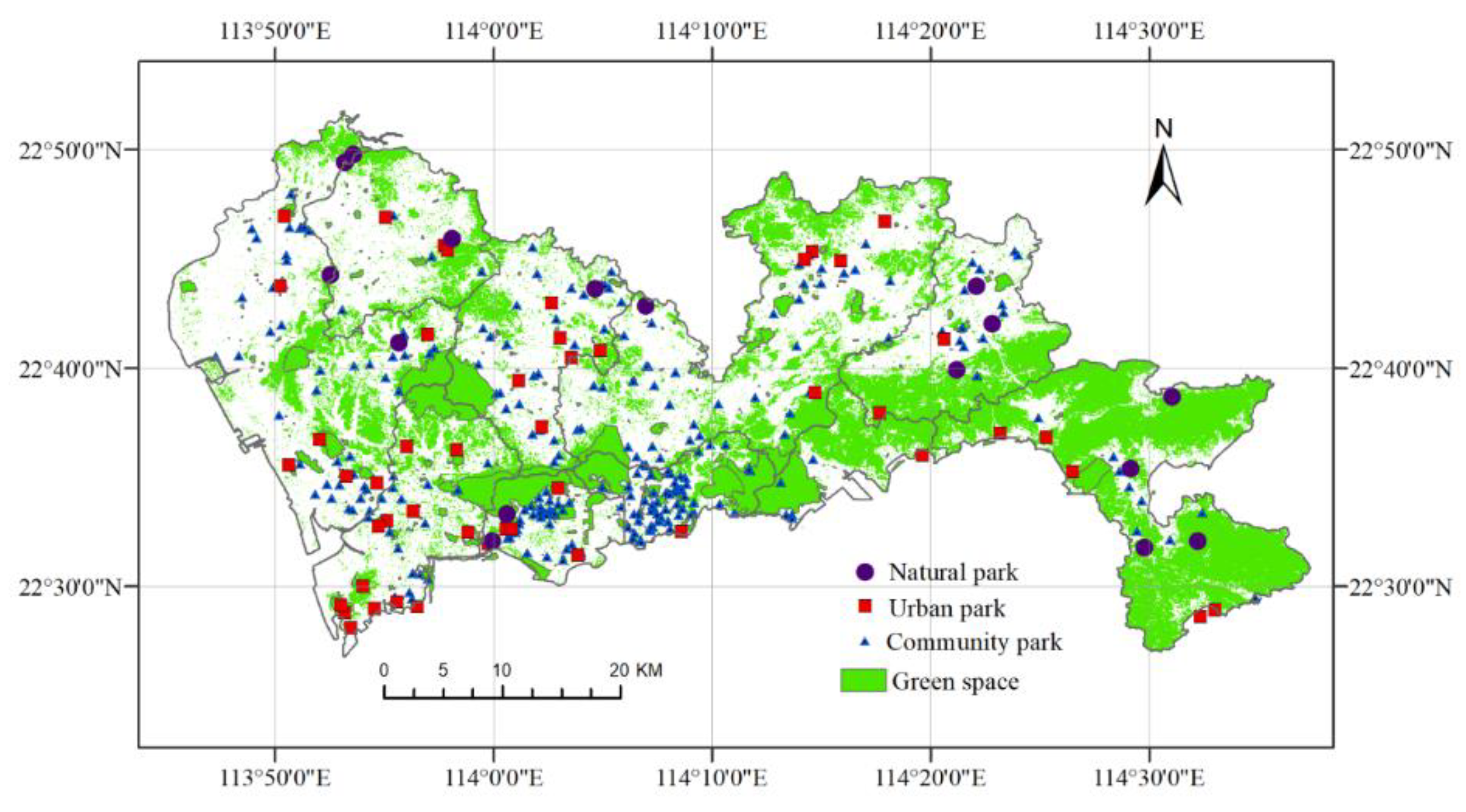
Land-use data for Shenzhen in 2017 were provided by The Global Ecosystems and Environment Observation Analysis Research Cooperation [46]. The land-use dataset was generated via remote sensing with high-resolution digital elevation models and night light data. The resolution was 30 m, with 10 land-use types. Eight types of land use in Shenzhen were identified: cropland, forest, grassland, shrubland, wetland, water, impervious surface, and bareland. Urban public green space includes parks and reserves, sporting fields, riparian areas such as streams and river banks, greenways and trails, community gardens, street trees, and nature conservation areas, as well as less conventional spaces such as green walls, green alleyways, and cemeteries [47]. In this study, UGS is defined as parks, wetlands, grasslands, and forests in Shenzhen. After identifying green spaces in Shenzhen with the land-use data, the Statistic Book for Green Parks in Shenzhen (May 2018 version; http://cgj.sz.gov.cn/zwgk/tjsj/zxtjxx/201805/t20180525_11941634.htm) was examined to extract the names, areas, and addresses of green parks [48]. Finally, the spatial boundaries or locations of listed green parks were drawn from OpenStreetMap (OSM) (https://www.openstreetmap.org/#map) and Amap (https://ditu.amap.com/). We searched for green parks listed in the Statistic Book for Green Parks in Shenzhen using OSM and Amap and identified their boundaries by altitude and longitude. The boundaries for each green park were converted to points using ArcGIS, after which they were converted to polygons. Only some of the green parks maintained boundary information in OSM and Amap, while other green parks were presented as points to reflect their locations. UGS in Shenzhen, comprising wetlands, grasslands, and forests, is presented in Figure 2.

2.2.2. Land Surface Temperature (LST) Retrieval

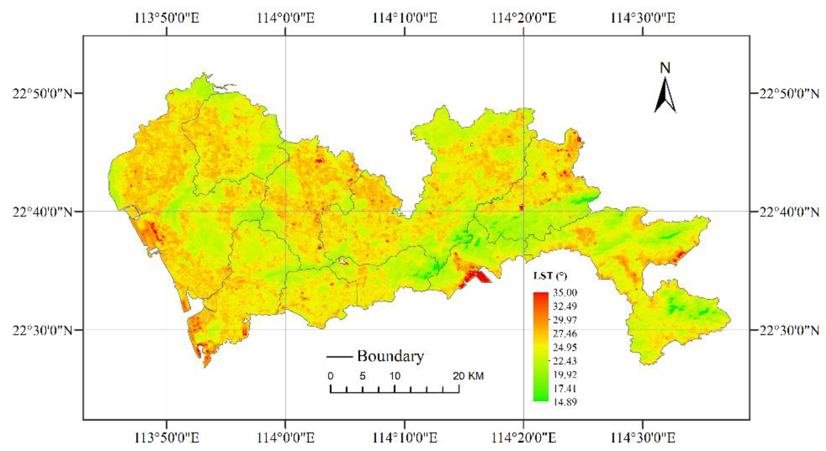
The Landsat 8 Thermal Infrared Sensor (TIRS) data were downloaded from the USGS Global Visualization Viewer (http://glovis.usgs.gov/), with a resolution of 30 m (on 1 and 23 October 2017) and a cloud cover of less than 1%. There are four commonly used methods for retrieving LST from thermal bands: (1) the multi-channel or split-window algorithm, (2) the multi-angle method, (3) the single-channel method, and (4) the radiative transfer equation [49]. In this study, the radiative transfer equation was used for Landsat 8 TIRS-10/11 to retrieve LSTs for Shenzhen. The main processes were defined with reference to Garcia-Santos [50]. The retrieved mean LSTs of Shenzhen on 1 and 23 October 2017 are displayed in Figure 3. Moreover, abnormal LST (higher than 45 degrees) occurred at the location of a waste incineration plant. This value was deleted and set as “no data”.

2.2.3. Point of Interest Retrieval

Points of interest (POIs) were retrieved from Amap, which is one of the largest desktop and mobile map service providers in China. Using Amap’s application programming interface, 9490 POI records were gathered on 23 December 2018. Data on train stations, subway stations, bus stations, scenery, schools, hospitals, and swimming pools were retrieved for economic value evaluation. Table 1 presents the categories and the number of POI records per category, and Figure 4 illustrates the spatial distribution of POI density.

2.2.4. Housing Rental Price Retrieval

In this study, the rental prices for residential houses were extracted from several real estate portals in China, including sz.fang.com, sz.zu.anjuke.com, www.sofang.com, sz.lianjia.com/zufang/, sz.ganji.com/wblist/zufang/, and sz.58.com/chuzu/, all of which had a large number of page views and visitors. We trawled 12,792 housing rental samples on 18 December 2018 and extracted the ID, location, rent price, area, number of bedrooms and halls, and whether the whole house or only a bedroom was being rented for each sample. To prepare the data for use, first, repeated samples from different portals were filtered to one record. Then, samples that were located outside of Shenzhen or that had nine or more bedrooms and halls were deleted. Third, samples with abnormal rent prices or with rent prices larger than or smaller than the mean ± 3 std . of the total rent prices were deleted. Finally, samples with the same community name and type were combined into one sample by determining the average rent price per unit area (yuan/sq. m) and average area. After this process, 5192 samples remained. The remaining samples were converted to points according to their location information (see Figure 5).

3. Methods

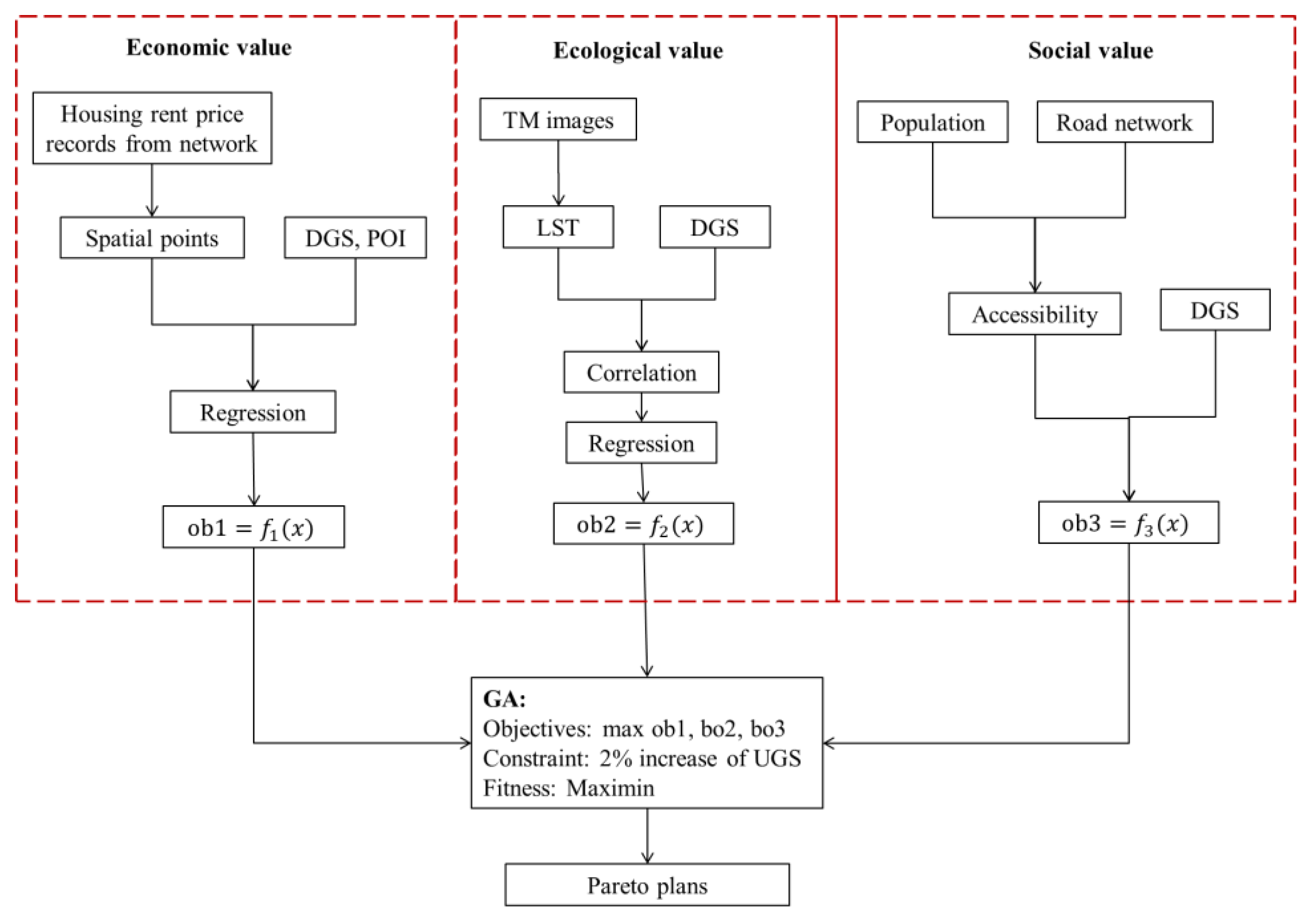
The framework of this study is presented in Figure 6. The economic value evaluation, ecological value evaluation, social value evaluation, and optimization model are presented in this section. Multi-objective optimization was carried out using a genetic algorithm.

3.1. Economic Value Evaluation

3.1.1. Evaluating Model

The hedonic prices model can be written as Equation (1) below:
P = f ( x 1 , x 2 , , x n ) ,
where P is housing rental prices or house prices, and x 1 , x 2 , …, x n are the factors that impact P . In Equation (1), f is the relationship between x and P , where the linear model, semi-log model, and double-log model were in existing studies. The linear model was used [37,51,52,53] in this study to evaluate the economic value of green spaces in Shenzhen.

3.1.2. Dependent and Independent Variables

The average rent prices of the 5191 house samples were set as the dependent variables. Then, the characteristics of the house, including its type and area, were set as two independent variables ( x 1 and x 2 , respectively). Specifically, the independent variables, the type of samples, were assigned positive integer values according to the number of bedrooms and halls of the sample (see Table 2).
Following the work of previous studies [37,54], each sample’s distance from a train station, distance from a subway station, density of schools, distance from a hospital, density of swimming pools, distance from scenery, distance from a river, distance from an urban park, rate of green space, and distance to a bus station were also selected as potential independent variables. All independent variables are listed in Table 3.
The buffering tool in ArcGIS was used to extract the distance-independent variables, including x 3 , x 4 , x 6 , x 8 , x 9 , x 10 , and x 12 (see Figure 7). On the other hand, density-independent variables, including x 5 , x 7 , and x 11 , were calculated with MATLAB. Specifically, the density of schools and density of swimming pools were indicated according to the number of schools or swimming pools in a circle scale, which were calculated with a radius of 200 m, 500 m, and 1000 m. The correlation analysis suggested that a radius of 1000 m was reasonable for reflecting the impact of schools and swimming pools on housing rental prices. The spatial distributions of x 3 to x 10 and x 12 are presented in Figure 7.
To determine the influence of distance of green space on rent prices, the density of green space (DGS) was calculated for square areas with a side length of 90 m, 150 m, …, and 1230 m. DGS was calculated according to Equation (2) below:
DGS d x = A r e a G S d x A r e a s q u a r e   d x ,
where A r e a G S d x is the area of green space in a square area and A r e a s q u a r e   d x is the area of the square area. Consequently, 20 regression models were built with different densities of green space, calculated using Equation (2) to determine a suitable length for calculating DGS. Several typical DGSs calculated with different square-area lengths (90 m, 390 m, 690 m, 990 m, and 1230 m) are presented in Figure 8.

3.2. Ecological Value Evaluation

The ability of green space to relieve LST or UHIs has been widely proven in existing studies [2,16,17,49]. In this study, we attempted to identify the impact of green space on LST and its impact distance for use in the UGS optimization system. First, correlation analysis between DGSs that were calculated at different scales and LST was carried out to determine the impact distance of green space on LST. The linear regression model was then built-up to quantize the relationship between DGS and LST.

3.2.1. Correlation Analysis

Correlation analysis between DGSs with different lengths and LST was carried out to identify the highest correlation and the impact distance as the length of DGS. Since LST is lower on mountains, the correlation analysis was carried out only for areas with elevations of lower than 300 m [55].

3.2.2. Evaluating Model

After the correlation analysis, we selected the DGSs with the highest R coefficient, with LST as the independent variable, to determine the relationship between green space and LST, as in Equation (3):
LST = f ( DGS d x ) .
In this study, the linear regression model was used as f in Equation (3).

3.3. Social Value Evaluation

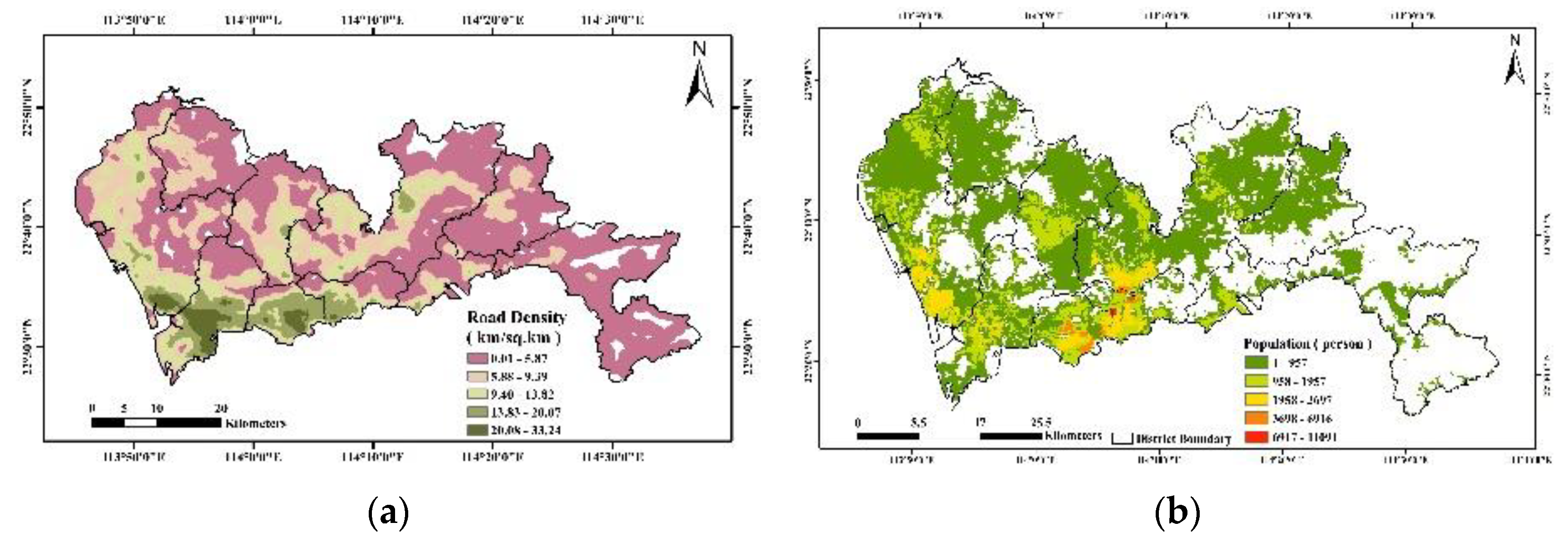
The social value of green space is determined by the amount of green space, the accessibility of such space, and the demand for green space. Therefore, the density of green space was used to indicate the amount of green space, the density of road networks was used to indicate accessibility, and the spatial distribution of the population was used to indicate the demand for green space. The social value of green space was calculated by Equation (4):
SO = DGS d x Density r o a d P o p ,
where Density r o a d is the density of road networks, and P o p is the population. Specifically, in calculating Density r o a d , high-speed roads, urban high-speed roads, railways, national roads, provincial roads, and other urban road networks were considered. The unit of Density r o a d is km per sq. km, and the density of road networks was calculated within 5 km (see Figure 9a). The spatial distribution of the population in Shenzhen in 2015 was gathered from the Global Human Settlement Layer (GHSL) data center with a resolution of 250 m by 250 m (see Figure 9b). The DGS was calculated with the length of one side at 510 m with reference to existing studies of green space accessibility calculations [13].

Multi-Objective Optimization

Three objectives were set to guide green space optimization. First, the distribution of green space should maximize the economic value by increasing local rent prices. Second, the distribution of green space should regulate the local climate in Shenzhen by relieving high LST. Third, green space should be located in places with high accessibility and high population density to maximize its social value. Meanwhile, the increasing amount of green space was set as the constraint. The objectives and constraints are shown below.
Ob1: Maximizing economic value of green space
Ob 1 = ( N D G S 690 DGS 690 ) a 1 HD
Ob2: Maximizing ecological value of green space
Ob 2 = ( DGS 270 N D G S 270 ) a 2 LST
Ob3: Maximizing social value of green space
Ob 3 = ( N D G S 510 DGS 510 ) AccMap
Constraint: Total increased green space must be less than ConP A r e a U G S , where N D G S d x is the density of UGS after optimization, and   a 1 and a 2 are the coefficients determined by Equation (1) and Equation (2). HD is the density of housing rental price sample points; LST is the land surface temperature of Shenzhen; and AccMap is the spatial distribution of accessibility. ConP is the ratio, and A r e a U G S is the area of UGS in Shenzhen.
Multi-objective optimization was carried out using GA. Built-up land in Shenzhen was coded as genes in the GA, which can be assigned a value of 0 or 1. An assignment of 0 indicates that the gene will not change into UGS, while 1 indicates that it will. All the coded genes constituted one chromosome, which can be thought of as one solution. One generation was represented by 100 chromosomes, presenting 100 alternative solutions, all of which satisfied the constraints. The values of the objectives were calculated. Then, selection, crossover, and mutation in the GA were carried out. In the selection process, the maximin fitness function [56] was used to calculate the fitness of one alternative solution. Two solutions that were randomly selected from the top ten solutions were set as parents in the GA. Then, crossover was carried out between genes in the GA to generate 100 new solutions. Moreover, a 0.05 probability of mutation was carried out to avoid local optimization. This means that there was a 0.05 probability that the newly generated genes would randomly covert to 0 or 1. The new 100 solutions were generated through a process of selection, crossover, and mutation until the iteration reached the threshold, which was set at 200. Moreover, new UGS should not exceed 2% of existing UGS in Shenzhen, meaning that ConP should be 0.02.

4. Results

4.1. The Economic Value of Green Space

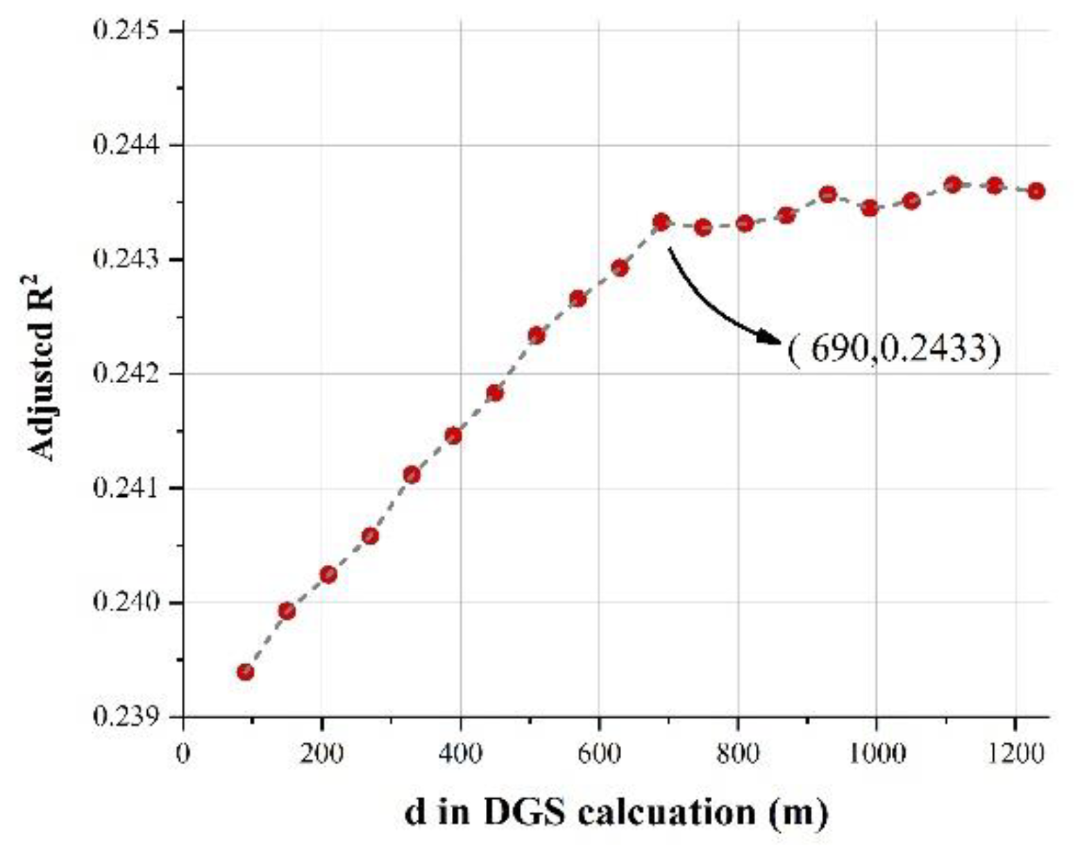
The results of regressions with different DGSs are presented in Table 4. The distance from a bus station ( x 12 ) was removed from some regression models, since its significance did not satisfy the requirements. As the results show, change in DGSs leads to variation in R-squared for models. Figure 10 illustrates the variation in R-squared along with different DGSs. It was found that when the DGS covered the square scale with one side length longer than 690 m, the impact of DGS on rent prices became stable at a high range (with an adjusted R-squared around 0.243). Therefore, in the process of optimizing green space, when economic objectives are considered, the optimization model should consider the impact of green spaces in a square scale with a side length of 690 m.
After identifying the influence scale, a univariate linear regression was built up to identify the impact of UGS on housing rental prices, as shown in Equation (8):
y = 24.9540 U G S 690 + 72.11 ,
where y is the dependent variable, housing rental prices, and UGS 690 is the rate of UGS in a square scale with a side length of 690 m. The R-squared is 0.0164, and p is 0. This suggests that the UGS can explain a 1.64% variation in housing rental prices, and the regression is significant.

4.2. The Ecological Value of Green Space

The correlation between DGSs and LST is illustrated in Figure 11. The results indicate that there was a negative relationship between green space and LST. This negative relationship became clearer (with an R of −0.74714) when the DGS considered the green space in a square area with a side length of 270 m.
According to the results presented in Figure 11, the selected DGS was used to build a univariate linear regression was built up to identify the impact of UGS on LST, as Equation (9) shows:
y = 3.3806 U G S 270 + 25.8474 ,
where y is the dependent variable, LST, and UGS 270 is the rate of UGS in a square scale with a side length of 270 m. The R-squared is 0.2321, and p is 0. This suggests that the UGS can explain a 23.21% variation in LST, and the regression is significant.

4.3. The Social Value of Green Space

The spatial distribution of accessibility was calculated on the basis of density of the road network and spatial distribution of the population (see Figure 9). The social value can be calculated as shown in Equation (10):
y = A c c D G S 510 ,
where y is social value; Acc is spatial distribution of accessibility; and DGS 510 is the spatial distribution of green space rate with a side of length 510 m.

4.4. Green Space Optimization for Shenzhen

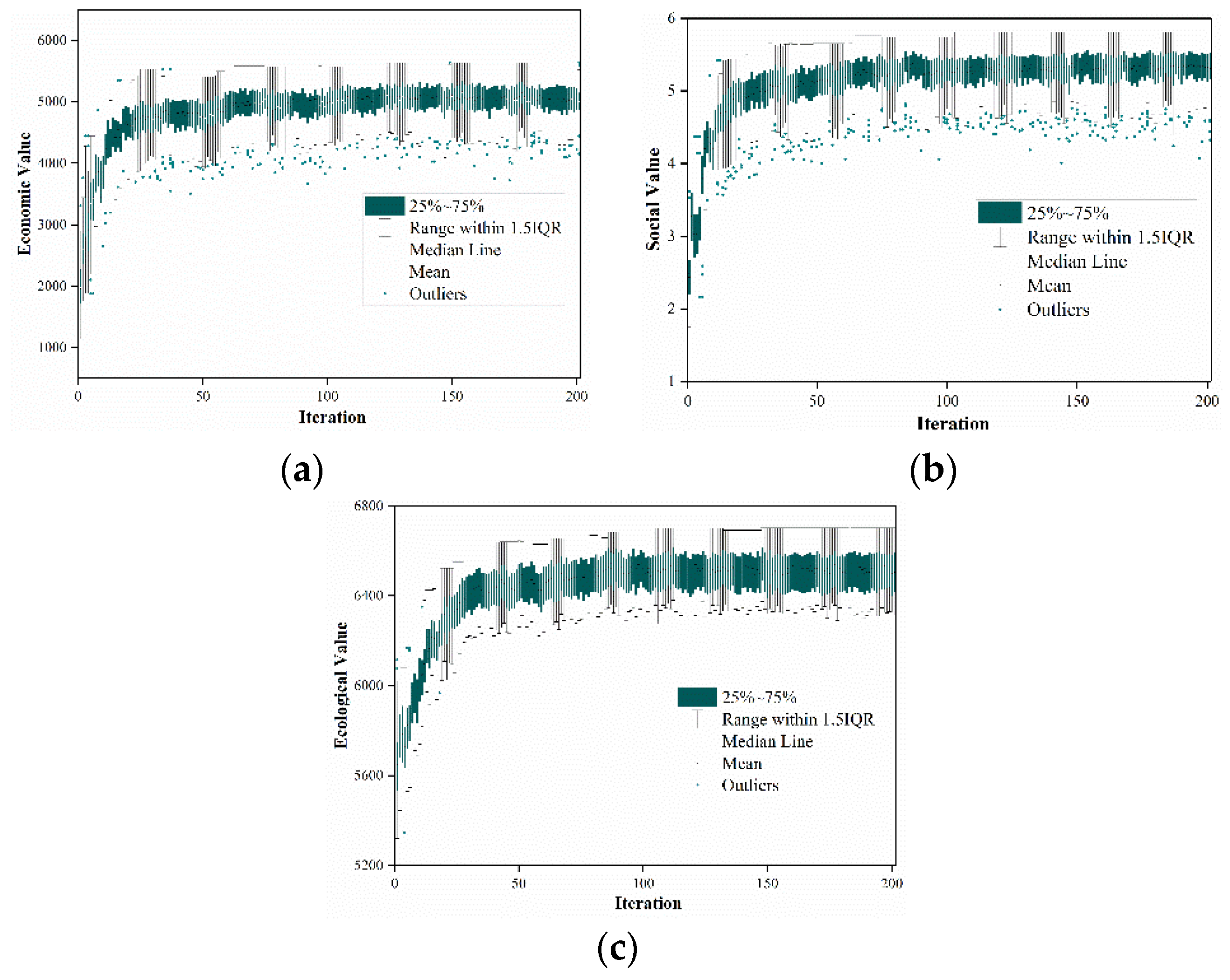
Optimization was based on the evaluations of economic, ecological, and social values of UGS. The variations of objective value with mean, median line, outliers, and 1.5* interquartile range (range within 1.5IQR) are presented in Figure 12 from the first generation to the last generation in the GA. The optimization showed that from the first generation to the last generation, economic value and ecological value clearly increased from the 1st to the 20th iteration. Thereafter, the objective value became stable, as shown in Figure 12a,b. The social value increased from the first generation to the 10th, and from then on the objective value became stable (see Figure 12c). The variations in objective value suggest that allocating green space in Shenzhen can improve economic, ecological, and social value.
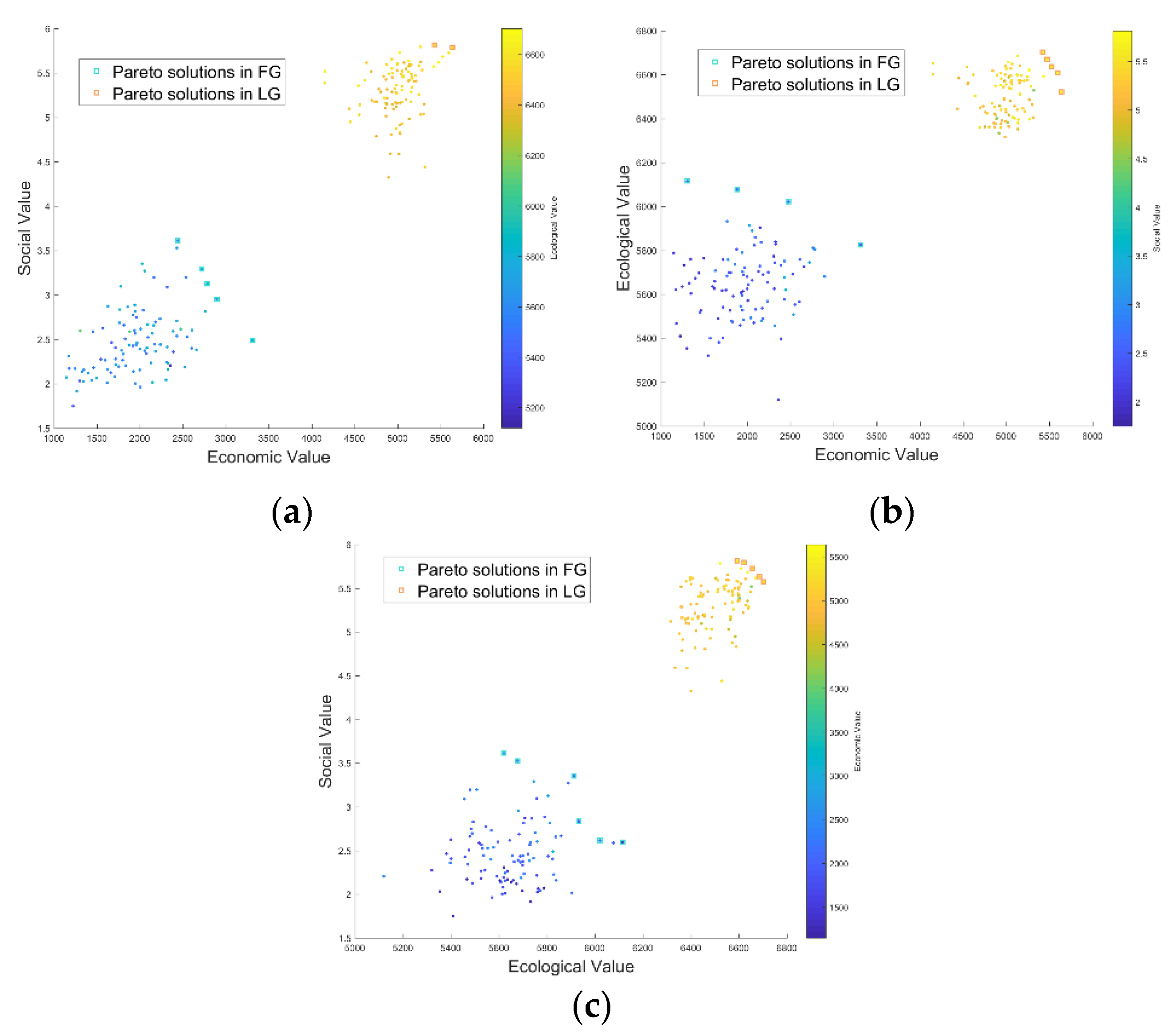
In addition to the variations in objective value, the Pareto solutions in the first and last generations are presented in Figure 13. We found that the solutions moved further away from the origin, indicating increases in objective value. The Pareto solutions dominated the other solutions.
Finally, the probability of optimized new UGS is presented in Figure 14. In the first generation, new increased UGSs were randomly spread around Shenzhen, with a relatively low probability (see Figure 14a). After optimization, the new increased UGSs were explicitly located with relatively high probability (see Figure 14b). As Figure 14b shows, the optimal UGS was often located in highly developed urban areas.

5. Discussion

In this paper, we estimated the economic, social, and ecological value of UGS in Shenzhen. Furthermore, we suggested a spatial planning method for UGS that satisfies the multiple requirements of simultaneously maximizing economic, social, and ecological value. The results indicate that MOP is a viable method for solving spatial problems in the establishment of UGS. Using MOP, Pareto solutions were detected, and the objectives were optimized. To identify the means of objective evaluation in MOP, the relationship between spatial distribution of UGS and its economic, social, and ecological value was analyzed. Specifically, the economic value of UGS was estimated using 5192 rent-price samples extracted from several major real estate portals in China. This method was cheaper and made it easier to maintain spatial information compared with traditional methods such as questionnaire surveys or field surveys. The ecological value of UGS was indicated by its relief of LST in urban areas. The social value of UGS was calculated on the basis of density of road network and spatial distribution of the population. The results suggest that UGS does affect housing rental prices in Shenzhen at a scale of 345 m. The relief of LST was a combined effect of UGS within 135 m. As for social value, a 255 m distance to enable travel by foot was selected to evaluate the accessibility of UGS in Shenzhen. Various affect distances of UGS for different values were identified. The affect distance of UGS should be clarified, and optimization carried out by considering affect distance.
After estimating the relationship between UGS and economic, ecological, and social value, MOP was carried out. The identified affect distances were put into the GA method to carry out the MOP for UGS in Shenzhen. The results indicate that MOP is a viable method for solving spatial problems in the establishment of UGS. From the first to the last generation, the economic value, ecological value, and social value of Shenzhen increased. However, there was no solution that simultaneously maintained the largest economic, ecological, and social value, which suggests that these three UGS values for Shenzhen may be conflicting. This is probably because maximizing economic value trends locate UGS in places with residential buildings, while maximizing ecological value and social value trends locate UGS in places with high urban heat island and population, respectively.
To date, MOP has been widely used in the field of land-use optimization where all land-use types are included. In this paper, merely one land-use type, UGS, was considered. This makes the optimization more explicit; the functions of green space can be fully estimated and the tradeoffs among different values can be considered. Because of the high economic, social, and ecological value of green space in urban areas, UGS planning or optimization has become popular in urban planning. This study proposed an optimization method that facilitates the Government’s management of UGS. The method proposed here also benefits residents by improving the value of UGS.
Several limitations exist in this study, which should be considered in future work. In urban systems, green spaces have various functions, including cooling, runoff reduction, and serving as ecological corridors; this study only considered three typical and popular functions of UGS. Future studies should consider more functions to reflect the full value of such spaces. Furthermore, in this study, we assumed that other land-use types were constant and that new green spaces would only be located in built-up areas. This is reasonable and reduces optimization costs; however, in future studies, optimization should be carried out by assuming that green space can be located on or close to built-up land. Working with this assumption, the system will generate more possible solutions for decision-makers.

Author Contributions

Data curation, Y.Y. and W.Z.; formal analysis, K.L.; investigation, P.F. and K.C.; resources, W.Z.; software, W.H.; validation, W.H. All authors have read and agreed to the published version of the manuscript.

Funding

Financial support was provided by the Open Fund of Key Laboratory of Urban Land Resources Monitoring and Simulation, MNR (Grant No. KF-2018-03-028); National Science Foundation of China (Grant No. 41601415 and 41877001); the Fundamental Research Funds For The Central Universities Grant No. 2662019PY074.

Conflicts of Interest

The authors declare no conflict of interest.

References

  1. Zhao, L.; Lee, X.; Smith, R.B.; Oleson, K. Strong contributions of local background climate to urban heat islands. Nature 2014, 511, 216–219. [Google Scholar] [CrossRef]
  2. Bao, T.; Li, X.; Zhang, J.; Zhang, Y.; Tian, S. Assessing the distribution of urban green spaces and its anisotropic cooling distance on urban heat island pattern in Baotou, China. ISPRS Int. J. Geo inf. 2016, 5, 12. [Google Scholar] [CrossRef]
  3. van den Berg, A.E.; Maas, J.; Verheij, R.A.; Groenewegen, P.P. Green space as a buffer between stressful life events and health. Soc. Sci. Med. 2010, 70, 1203–1210. [Google Scholar] [CrossRef] [PubMed] [Green Version]
  4. Chen, Y.Y.; Liu, X.P.; Gao, W.X.; Wang, R.Y.; Li, Y.; Tu, W. Emerging social media data on measuring urban park use. Urban. For. Urban. Green. 2018, 31, 130–141. [Google Scholar] [CrossRef]
  5. Xu, M.; Xin, J.; Su, S.; Weng, M.; Cai, Z. Social inequalities of park accessibility in Shenzhen, China: The role of park quality, transport modes, and hierarchical socioeconomic characteristics. J. Transp. Geogr. 2017, 62, 38–50. [Google Scholar] [CrossRef]
  6. Pearce, D. Nature’s services. Societal dependence on natural ecosystems—Daily, GC. Science 1997, 277, 1783. [Google Scholar] [CrossRef]
  7. Hong, W.; Guo, R. Indicators for quantitative evaluation of the social services function of urban greenbelt systems: A case study of Shenzhen, China. Ecol. Indic. 2017, 75, 259–267. [Google Scholar] [CrossRef]
  8. Maas, J.; Verheij, R.A.; de Vries, S.; Spreeuwenberg, P.; Schellevis, F.G.; Groenewegen, P.P. Morbidity is related to a green living environment. J. Epidemiol. Commun. H 2009, 63, 967–973. [Google Scholar] [CrossRef] [Green Version]
  9. Villeneuve, P.J.; Jerrett, M.; Su, J.G.; Burnett, R.T.; Chen, H.; Wheeler, A.J.; Goldberg, M.S. A cohort study relating urban green space with mortality in Ontario, Canada. Environ. Res. 2010, 115, 51–58. [Google Scholar] [CrossRef]
  10. Alexander, D.S.; Huber, R.L.; Piper, C.R.; Tanner, A.E. The association between recreational parks, facilities, and childhood obesity: A cross-sectional study of the 2007 National Survey of Children’s Health. J. Epidemiol. Community Health 2013, 67, 427–431. [Google Scholar] [CrossRef] [Green Version]
  11. Troy, A.R.; Grove, J.M.; O’Neill-Dunne, J.P.M.; Pickett, S.T.A.; Cadenasso, M.L. Predicting opportunities for greening and patterns of vegetation on private urban lands. J. Environ. Manag. 2007, 40, 394–412. [Google Scholar] [CrossRef] [PubMed]
  12. Wang, Q.; Zhang, Z. Examining social inequalities in urban public leisure spaces provision using principal component analysis. Qual. Quant. 2017, 51, 2409–2420. [Google Scholar] [CrossRef]
  13. Song, Y.; Huang, B.; Cai, J.; Chen, B. Dynamic assessments of population exposure to urban greenspace using multi-source big data. Sci. Total Environ. 2018, 634, 1315–1325. [Google Scholar] [CrossRef] [PubMed]
  14. Nesbitt, L.; Meitner, M.J.; Girling, C.; Sheppard, S.R.J.; Lu, Y. Who has access to urban vegetation? A spatial analysis of distributional green equity in 10 US cities. Landsc. Urban. Plan. 2019, 181, 51–79. [Google Scholar] [CrossRef]
  15. Li, W.; Saphores, J.M.; Gillespie, T.W. A comparison of the economic benefits of urban green spaces estimated with NDVI and with high-resolution land cover data. Landsc. Urban. Plan. 2015, 133, 105–117. [Google Scholar] [CrossRef]
  16. Qiu, G.Y.; Zou, Z.; Li, X.; Li, H.; Guo, Q.; Yan, C.; Tan, S. Experimental studies on the effects of green space and evapotranspiration on urban heat island in a subtropical megacity in China. Habitat Int. 2017, 68, 30–42. [Google Scholar] [CrossRef]
  17. Xiao, X.D.; Dong, L.; Yan, H.; Yang, N.; Xiong, Y. The influence of the spatial characteristics of urban green space on the urban heat island effect in Suzhou Industrial Park. Sustain. Cities. Soc. 2018, 40, 428–439. [Google Scholar] [CrossRef]
  18. Nowak, D.J.; Civerolo, K.L.; Rao, S.T.; Sistla, G.; Luly, C.J.; Crane, D.E. A modeling study of the impact of urban trees on ozone. Atmos. Environ. 2000, 34, 1601–1613. [Google Scholar] [CrossRef]
  19. Nowak, D.J.; Crane, D.E.; Stevens, J.C. Air pollution removal by urban trees and shrubs in the United States. Urban. For. Urban. Green. 2006, 4, 115–123. [Google Scholar] [CrossRef]
  20. Escobedo, F.J.; Nowak, D.J. Spatial heterogeneity and air pollution removal by an urban forest. Landsc. Urban. Plan. 2009, 90, 102–110. [Google Scholar] [CrossRef]
  21. Nowak, D.J.; Crane, D.E. Carbon storage and sequestration by urban trees in the USA. Environ. Pollut. 2002, 116, 381–389. [Google Scholar] [CrossRef]
  22. Morancho, A.B. A hedonic valuation of urban green areas. Landsc. Urban. Plan. 2003, 66, 35–41. [Google Scholar] [CrossRef]
  23. Luttik, J. The value of trees, water, and open space as reflected by house prices in the Netherlands. Landsc Urban. Plan. 2000, 48, 161–167. [Google Scholar] [CrossRef]
  24. Jim, C.Y.; Chen, W.Y. External effects of neighborhood parks and landscape elements on high-rise residential value. Land Use Policy 2010, 27, 662–670. [Google Scholar] [CrossRef]
  25. Bolitzer, B.; Netusil, N.R. The impact of open spaces on property values in Portland, Oregon. J. Environ. Manag. 2000, 59, 185–193. [Google Scholar] [CrossRef]
  26. Poudyal, N.C.; Hodges, D.G.; Merrett, C.D. A hedonic analysis of the demand for and benefits of urban recreation parks. Land Use Policy 2009, 26, 975–983. [Google Scholar] [CrossRef]
  27. Huang, C.; Huang, P.; Wang, X.; Zhou, Z. Assessment and optimization of green space for urban transformation in resources-based city—A case study of Lengshuijiang city, China. Urban. For. Urban. Green. 2018, 30, 295–306. [Google Scholar] [CrossRef]
  28. Zhang, Y.J.; Murray, A.T.; Murray, B.L. Optimizing green space locations to reduce daytime and nighttime urban heat island effects in Phoenix, Arizona. Landsc. Urban. Plan. 2017, 165, 162–171. [Google Scholar] [CrossRef]
  29. Unal, M.; Uslu, C. Evaluating and optimizing urban green spaces for compact urban areas: Cukurova District in Adana, Turkey. ISPRS Int. J. Geoinf. 2018, 7, 70. [Google Scholar] [CrossRef] [Green Version]
  30. Yoon, E.J.; Kim, B.; Lee, D.K. Multi-objective planning model for urban greening based on optimization algorithms. Urban. For. Urban. Green. 2019, 40, 183–194. [Google Scholar] [CrossRef]
  31. Zhang, W.; Huang, B. Soil erosion evaluation in a rapidly urbanizing city (Shenzhen, China) and implementation of spatial land-use optimization. Environ. Sci. Pollut. Res. 2014, 22, 4475–4490. [Google Scholar] [CrossRef] [PubMed]
  32. Cao, K.; Huang, B.; Wang, S.; Lin, H. Sustainable Land Use Optimization Using Boundary-based Fast Genetic Algorithm. Comput. Environ. Urban Syst. 2012, 36, 257–269. [Google Scholar] [CrossRef]
  33. Cao, K.; Batty, M.; Huang, B.; Liu, Y.; Yu, L.; Chen, J. Spatial Multi-objective Land Use Optimization: Extensions to the Non-dominated Sorting Genetic Algorithm-II. Inter. J. Geogr. Inf. Sci. 2011, 25, 1949–1969. [Google Scholar] [CrossRef]
  34. Steuer, R.E. Multiple Criteria Optimization: Theory, Computation, and Application; Wiley: Hoboken, NJ, USA, 1989. [Google Scholar]
  35. Miettinen, K. Nonlinear Multiobjective Optimization; Springer: Berlin/Heidelberg, Germany, 1999. [Google Scholar]
  36. Cao, K.; Zhang, W.; Liu, S.; Huang, B.; Huang, W. Pareto law-based regional inequality analysis of PM2.5 air pollution and economic development in China. J. Environ. Manag. 2019, 252, 109635. [Google Scholar] [CrossRef]
  37. Kong, F.; Yin, H.; Nakagoshi, N. Using GIS and landscape metrics in the hedonic price modeling of the amenity value of urban green space: A case study in Jinan City, China. Landsc. Urban. Plan. 2007, 79, 240–252. [Google Scholar] [CrossRef]
  38. You, H. Characterizing the inequalities in urban public green space provision in Shenzhen, China. Habitat Int. 2016, 56, 176–180. [Google Scholar] [CrossRef]
  39. Li, Q.; Yu, Y.; Jiang, X.; Guan, Y. Multifactor-based environmental risk assessment for sustainable use planning in Shenzhen, China. Sci. Total Environ. 2019, 657, 1051–1063. [Google Scholar] [CrossRef] [PubMed]
  40. Gong, C.; Yu, S.; Chen, J. Spatiotemporal dynamics of urban forest conversion through model urbanization in Shenzhen, China. Int. J. Remote Sens. 2011, 32, 9071–9092. [Google Scholar] [CrossRef]
  41. Gong, C.; Chen, J.; Yu, S. Biotic homogenization and differentiation of the flora in artificial and near-natural habitats across urban green spaces. Landsc. Urban. Plan. 2013, 120, 158–169. [Google Scholar] [CrossRef]
  42. Zheng, C.; Cao, C.; Cheng, J.; Wu, Y.; Xie, X.; Xu, M. A study on land use and land cover change during urbanization in Shenzhen using data from Chinese satellites. Sci. Sin. 2011, 41, 140–152. [Google Scholar] [CrossRef]
  43. Chen, Z.; Gong, C.; Wu, J.; Yu, S. The influence of socioeconomic and topographic factors on nocturnal urban heat islands: A case study in Shenzhen, China. Int. J. Remote Sens. 2012, 33, 3834–3849. [Google Scholar] [CrossRef]
  44. Burak, G.; Seto, K.C. Environmental impacts of urban growth from an integrated dynamic perspective: A case study of Shenzhen, South China. Glob. Environ. Chang. 2008, 18, 0–735. [Google Scholar]
  45. Li, L.; Du, Q.; Ren, F.; Ma, X. Assessing spatial accessibility to hierarchical urban parks by multi-types of travel distance in Shenzhen, China. Int. J. Environ. Res. Public Health 2019, 16, 1038. [Google Scholar] [CrossRef] [PubMed] [Green Version]
  46. The Global Ecosystems and Environment Observation Analysis Research Cooperation. Available online: http://data.ess.tsinghua.edu.cn/ISLandCoverAfrica.html (accessed on 12 December 2018).
  47. Wolch, J.R.; Byrne, J.; Newell, J.P. Urban green space, public health, and environmental justice: The challenge of making cities “just green enough”. Landsc. Urban. Plan. 2014, 125, 234–244. [Google Scholar] [CrossRef] [Green Version]
  48. Urban Management and Comprehensive Law Enforcement Bureau of Shenzhen. Statistic Book for Green Parks in Shenzhen. 2018. Available online: http://cgj.sz.gov.cn/zwgk/tjsj/zxtjxx/201805/t20180525_11941634.htm (accessed on 25 December 2018).
  49. Naeem, S.; Cao, C.; Qazi, W.A.; Zamani, M.; Wei, C.; Acharya, B.K.; Rehman, A.U. Studying the association between green space characteristics and land surface temperature for sustainable urban environments: An analysis of Beijing and Islamabad. ISPRS Int. J. Geo Inf. 2018, 7, 38. [Google Scholar] [CrossRef] [Green Version]
  50. Garcia-Santos, V.; Cuxart, J.; Martinez-Villagrasa, D.; Jimenez, M.A.; Simo, G. Comparison of three methods for estimating land surface temperature from Landsat 8-TIRS sensor data. Remote Sens. 2018, 10, 1450. [Google Scholar] [CrossRef] [Green Version]
  51. Witte, A.D.; Sumka, H.J.; Erekson, H. An estimate of a structural hedonic price model of the housing market: An application of Rosen’s theory of implicit markets. Econometrica 1979, 47, 1151–1173. [Google Scholar] [CrossRef] [Green Version]
  52. Saphores, J.D.; Li, W. Estimating the value of urban green areas: A hedonic pricing analysis of the single-family housing market in Los Angeles, CA. Landsc. Urban. Plan. 2012, 104, 373–387. [Google Scholar] [CrossRef]
  53. Panduro, T.E.; Veie, K.L. Classification and valuation of urban green spaces: A hedonic house price valuation. Landsc. Urban. Plan. 2013, 120, 119–128. [Google Scholar] [CrossRef]
  54. Chen, W.Y. Environmental externalities of urban river pollution and restoration: A hedonic analysis in Guangzhou (China). Landsc. Urban. Plan. 2017, 157, 170–179. [Google Scholar] [CrossRef]
  55. Wu, Z.; Zhang, Y. Spatial variation of urban thermal environment and its relation to green space patterns: Implication to sustainable landscape planning. Sustainability 2018, 10, 2249. [Google Scholar] [CrossRef] [Green Version]
  56. Balling, R. The Maximin Fitness Function; Multi-objective City and Regional Planning. International conference on Evolutionary Multi-Criterion Optimization; Springer: Berlin, Germany, 2003; pp. 1–15. [Google Scholar]
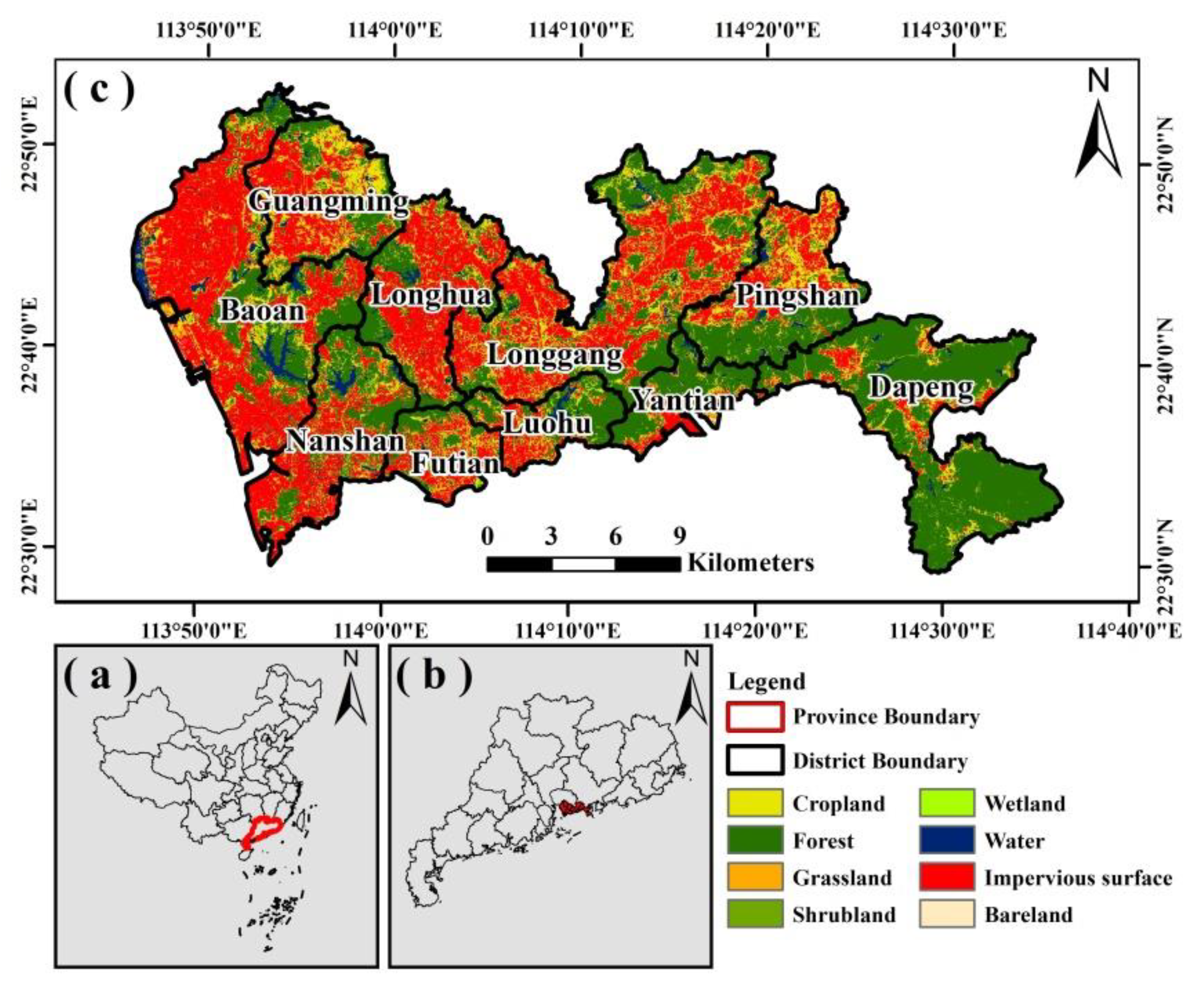
Figure 1. (a) The location of Guangdong Province in China; (b) the location of Shenzhen in Guangdong Province; and (c) the land-use pattern of Shenzhen in 2017.
Sustainability 12 01844 g001
Figure 2. The spatial distribution of urban green space (UGS) in Shenzhen.
Sustainability 12 01844 g002
Figure 3. The mean land surface temperature (LST) of Shenzhen on 1 and 23 October 2017.
Sustainability 12 01844 g003
Figure 4. The spatial distribution of POI density for Shenzhen (23 December 2018).
Sustainability 12 01844 g004
Figure 5. Spatial distribution of sample points and rent prices (yuan/sq. m).
Sustainability 12 01844 g005
Figure 6. Framework of this study.
Sustainability 12 01844 g006
Figure 7. The spatial distributions of independent variables from x 3 to x 10 and x 12 .
Sustainability 12 01844 g007
Figure 8. DGS (density of green space) with a distance of (a) 90 m, (b) 390 m, (c) 690 m, (d) 990 m, and (e) 1230 m.
Sustainability 12 01844 g008
Figure 9. The spatial distributions of (a) density of road networks, (b) population, and (c) accessibility in Shenzhen.
Sustainability 12 01844 g009aSustainability 12 01844 g009b
Figure 10. Variations of adjusted R-squared along with different DGSs.
Sustainability 12 01844 g010
Figure 11. Correlations between LST and rate of DGS.
Sustainability 12 01844 g011
Figure 12. Variation of objective value from the first to the last iteration in the genetic algorithm: (a) economic value, (b) ecological value, and (c) social value.
Sustainability 12 01844 g012
Figure 13. Pareto solutions in the first and last generations. (a) Pareto solutions for social value and economic value, (b) Pareto solutions for economic value and ecological value, and (c) Pareto solutions for ecological value and social value.
Sustainability 12 01844 g013
Figure 14. Spatial distribution of new increased green space in (a) the first generation and in (b) the Pareto solutions of the last generation.
Sustainability 12 01844 g014
Table 1. Categories and numbers of retrieved points of interest (POIs).
CategoryNumberRetrieval Date
Train station1323 December 2018
Subway station327
Bus station 5049
Scenery2081
School1240
Hospital380
Swimming pool400
Sum 9490
Table 2. Types for the samples of rent price and corresponding assigned value.
TypeValue
1 bedroom1
1 bedroom with 1 hall2
2 bedrooms with 1 hall3
2 bedrooms with 2 halls4
3 bedrooms with 1 hall5
3 bedrooms with 2 halls 6
4 bedrooms with 2 halls7
5 bedrooms with 2 halls8
Table 3. The selected independent variables.
NameVariablesDescription
x 1 AreaArea (sq. m) of room or house for samples.
x 2 TypeThe number of bedrooms and halls of samples.
x 3 Distance from train stationEuclidean distance from the sample point to the closest train station.
x 4 Distance from subway station Euclidean distance from the sample point to the closest subway station.
x 5 Density of schoolsDensity of schools at the location of the sample.
x 6 Distance from hospital Euclidean distance from the sample point to the closest hospital.
x 7 Density of swimming poolsDensity of swimming pools at the location of the sample.
x 8 Distance from scenery Euclidean distance from the sample point to the closest scenery.
x 9 Distance from riverEuclidean distance from the sample point to the closest river.
x 10 Distance from urban parkEuclidean distance from the sample point to the closest urban park.
x 11 Density of green spaceDensity of green space at the location of the sample.
x 12 Distance from bus station Euclidean distance from the sample point to the closest bus station.
Table 4. Estimated coefficients for linear regression model.
Length (meter)Model1Model2Model3Model4Model5Model6Model7Model8Model9Model10Model11Model12Model13Model14Model15Model16Model17Model18Model19Model20
 
90-
150 0.0227 *
210 0.0299 *
270 0.0372 *
330 0.0532 *
390 0.0597 *
450 0.0656 *
510 0.0726 *
570 0.0777 *
630 0.0822 *
690 0.0879 *
750 0.0883 *
810 0.0891 *
870 0.0902 *
930 0.0926 *
990 0.0923 *
1050 0.0936 *
1110 0.0956 *
1170 0.0963 *
1230 0.0970 *
x 1 0.2469 *0.2463 *0.2459 *0.2454 *0.2462 *0.2458 *0.2453 *0.2449 *0.2448 *0.2442 *0.2436 *0.2437 *0.2435 *0.2434 *0.2434 *0.2437 *0.2439 *0.2439 *0.2438 *0.2440 *
x 2 −0.0650 *−0.0654 *−0.0655 *−0.0656 *−0.0668 *−0.0667 *−0.0667 *−0.0666 *−0.0667 *−0.0667 *−0.0666 *−0.0666 *−0.0662 *−0.0660 *−0.0658 *−0.0655 *−0.0653 *−0.0651 *−0.0647 *−0.0650 *
x 3 −0.2449 *−0.2428 *−0.2421 *−0.2413 *−0.2387 *−0.2380 *−0.2372 *−0.2361 *−0.2353 *−0.2345 *−0.2337 *−0.2334 *−0.2331 *−0.2328 *−0.2322 *−0.2321 *−0.2318 *−0.2314 *−0.2312 *−0.2310 *
x 4 −0.2207 *−0.2228 *−0.2236 *−0.2250 *−0.2276 *−0.2285 *−0.2287 *−0.2292 *−0.2295 *−0.2293 *−0.2296 *−0.2292 *−0.2293 *−0.2294 *−0.2296 *−0.2294 *−0.2294 *−0.2298 *−0.2301 *−0.2301 *
x 5 −0.1207 *−0.1191 *−0.1183 *−0.1174 *−0.1162 *−0.1154 *−0.1146 *−0.1137 *−0.1129 *−0.1122 *−0.1115 *−0.1113 *−0.1110 *−0.1107 *−0.1103 *−0.1103 *−0.1101 *−0.1098 *−0.1097 *−0.1096 *
x 6 −0.0376−0.0404 *−0.0414 *−0.0418 *−0.0412 *−0.0423 *−0.0432 *−0.0440 *−0.0444 *−0.0449 *−0.0458 *−0.0462 *−0.0466 *−0.0468 *−0.0471 *−0.0471 *−0.0472 *−0.0474 *−0.0475 *−0.0477 *
x 7 0.1561 *0.1565 *0.1567 *0.1568 *0.1552 *0.1558 *0.1566 *0.1576 *0.1583 *0.1590 *0.1598 *0.1601 *0.1603 *0.1608 *0.1613 *0.1616 *0.1621 *0.1626 *0.1630 *0.1633 *
x 8 −0.0854 *−0.0829 *−0.0822 *−0.0815 *−0.0795 *−0.0791 *−0.0785 *−0.0778 *−0.0774 *−0.0772 *−0.0769 *−0.0769 *−0.0766 *−0.0764 *−0.0760 *−0.0759 *−0.0756 *−0.0753 *−0.0751 *−0.0748 *
x 9 −0.1391 *−0.1413 *−0.1418 *−0.1423 *−0.1436 *−0.1441 *−0.1448 *−0.1455 *−0.1461 *−0.1465 *−0.1470 *−0.1472 *−0.1475 *−0.1478 *−0.1482 *−0.1484 *−0.1488 *−0.1493 *−0.1497 *−0.1500 *
x 10 −0.1129 *−0.1066 *−0.1045 *−0.1024 *−0.0996 *−0.0979 *−0.0962 *−0.0942 *−0.0931 *−0.0920 *−0.0906 *−0.0903 *−0.0898 *−0.0891 *−0.0883 *−0.0883 *−0.0880 *−0.0873 *−0.0870 *−0.0868 *
x 11 0.0363 *0.0304 *0.02840.0267----------------
Constant0.48110.47730.47610.47470.47760.47610.47440.47210.47050.46930.46760.46710.46640.46550.46420.46370.46280.46160.46090.4606
Adjusted   R 2 0.23940.23990.24020.24060.24110.24150.24180.24230.24270.24290.24330.24330.24330.24340.24360.24340.24350.24370.24360.2436
* p < 0.05.