Mapping Urbanization and Evaluating Its Possible Impacts on Stream Water Quality in Chattanooga, Tennessee, Using GIS and Remote Sensing

Abstract

Impervious surfaces (IS) produced by urbanization can facilitate pollutants’ movement to nearby water bodies through stormwater. This study mapped and estimated the IS changes in Chattanooga, Tennessee, using satellite imagery acquired in 1986 and 2016. A model was developed utilizing the Normalized Difference Vegetation Index coupled with density slicing to detect and map urbanization through IS growth. Urban growth was quantified at USGS HUC12 watershed level including stream riparian areas. The obtained results show a net growth of 45.12 km² of IS with a heterogeneous distribution. About 9.96 km² of this growth is within 90 m of streams, about 6% of the study site’s land cover. The Lower South Chickamauga Creek watershed experienced the largest urban growth with a change from 24.2 to 48.5 km². Using the riparian zone percent imperviousness, a stream risk assessment model was developed to evaluate potential stream impairment due to this growth. Approximately 87, 131, and 203 km lengths of streams identified as potentially at high, very high, and extreme risks, respectively, to be impaired due to urban growth from the last 30 years. These findings would benefit to proactively implement sustainable management plans for the streams near rapidly urbanizing areas in the study site.

1. Introduction

Urban areas are often defined by anthropogenically created impervious surfaces such as concrete, asphalt, and metal [1,2]. Global urbanized areas, as of 2014, contain 54% of the global population and are estimated to increase to 66% by 2050. The rates of urbanization are not globally uniform. For example, in North America, 82% of the population resides in urban areas compared to other continents such as Africa and Asia with 40% and 48%, respectively. On the other hand, increases in urbanization are not consistent. The fastest growing areas are in Africa and Asia and are estimated to increase to 56% and 64%, respectively, with more urbanized areas such as Northern America growing at slower rates [3]. While slower than other areas globally, North America, and specifically the continental United States, is still experiencing significant growth both in urban population and urban development.

With urbanization continuing to increase, it has been imperative to monitor, manage, and research issues that could be associated with urban growth. An immense quantity of scientific literature has demonstrated the negative impacts of urban growth on resources such as agriculture, timber, surface and groundwater quality, and energy resources [4,5,6,7,8,9,10,11,12,13,14,15,16,17].

1.1. Urbanization and Surface Water Quality

As urban areas continue to densify and expand into their surrounding environment, their new development can alter the nearby landscape dynamics. Often these expanding urban areas encompass or encroach nearby surface water resources [18]. This spatial relationship between urban areas and water resources has long had the attention of the scientific community, whose work has shown that urban development can impact local surface water resources [19,20,21,22], especially the quality of water, as we can see in

Table 1. Selected water quality variable associations with urbanized land cover types.

Water Quality Variable	Land Cover Association	Parameter Concentration	Literature
Total suspended solids (TSS)	General Urban, IS	+	[23,24,25]
Turbidity	General Urban	+	[25,26,27]
Dissolved solids	Commercial	+	[20,25,28]
Dissolved oxygen (DO)	General Urban, IS, Residential, Commercial	-	[18,29,30,31]
Heavy metals	General Urban, Residential, Commercial, Industrial	+	[32,33,34]
Conductivity	General Urban, IS, Commercial, Residential and Agricultural	+	[29,35,36]
Temperature	General Urban, IS	+	[36,37,38]
pH	General Urban, IS	+	[36,39,40]
Total nitrogen (TN)	Commercial, Residential and Agricultural	+	[26,29,30]
Total phosphorus	Residential	+	[28,29,31]
Ammonia	General Urban	+	[33,41,42]
E. coli	General Urban, IS	+	[36,43,44]
Algae (chlorophyll)	Urban General, IS	+	[45,46,47]
Fecal coliform	General Urban, IS, Commercial, Residential and Agricultural	+	[24,29,43]

Note: The relationship is given by the general impact of the land cover on the parameter. A positive (+) or negative (-) symbol shows the parameter concentration response to increases in specified land cover. IS = Impervious Surfaces.

. All parameters listed in Table 1 have been found to be adversely affected by the listed land use types; with measured parameter levels all being higher than natural levels, (except dissolved oxygen which is found to be lower). Overall, urbanized watersheds have been found to have significant impacts on surface water resources including degraded water quality, habitat and biota. It is, therefore, crucial to monitor and investigate the quality of surrounding water resources near rapidly urbanizing areas to proactively implement water resource management plans.

1.2. Land Use and Land Cover Change (LULC) and Urbanization

Urban growth is the change in LULC for and by anthropogenic activities such as residential, commercial and industrial development. It is commonly quantified through LULC detection and analysis of selected classes such as agricultural, open field, urban, forest, wetland, and barren areas. Quantitatively assessing urban growth requires defining which LULC categories should be considered urban. For the USGS National Land Cover Database [48,49,50], urban land cover is defined by spatial intensity of developed land, which is the percentage of impervious surface (IS) per unit area. Other efforts to map urban growth involve using the amount of detectable IS to measure urban extent [51,52,53,54]. Impervious surfaces are defined as being composed of materials such as asphalt, concrete, and metal that slow or inhibit water infiltration to topsoil. Therefore, these surfaces include building rooftops, sidewalks, parking lots, and roads, and the amount of land cover composed of IS can then be related to urban growth.

Remote sensing has been established as an effective method for investigating urban growth due to the differing visible and spectral differences between LULC classes [55,56,57,58,59]. Urban growth detection using remote sensing has been used to investigate changes across a range of temporal and spatial scales due to the advantages offered by various remote sensing technologies. Through these investigations, numerous image processing techniques have been developed or utilized to improve LULC research precisions including: Tasseled Cap Transformation (TCT), Normalized Difference Built-Up Index (NDBI), Index-based Built-Up Index (IBI), Normalized Difference Vegetation Index (NDVI), and supervised classification schemes such as density slicing [56,60,61,62,63,64,65,66]. Impervious surface growth has been investigated using remote sensing and is often paired with water quality investigations due to the established relationship between the two variables [67,68,69].

1.3. Urban Growth and Riparian Areas

The land immediately surrounding water resources is considered riparian areas. These zones can be described as a range of area adjacent to water resources including areas 100 m away and further [70]. The conservation and protection of forest riparian land is critical as they act as buffers between the flows of matter from upland areas into hydrologic resources and have a strong influence on the surrounding water resource quality [71]. They are attributed with mitigating the flow of sediment and nutrients from surface and groundwater into adjacent water resources [72], effects on fish assemblages [73], and other physiochemical water quality variables [74,75]. As with other critical habitats, LULC development poses a significant threat to riparian areas by compromising the buffer’s ecological integrity and altering buffer areas’ landscape [76,77]. Research has suggested that vegetated buffers of a minimum of 30 m is needed to act as a functioning non-point source pollutant control [78].

Acting as a non-point source pollutant, IS proximity to water resources and the respective riparian buffer have also been found to affect water quality [78,79,80]. Riparian buffer LULC can have a better ability to predict stream surface water quality leading to an increase in research and government attention to understanding and protecting these corridors [81,82]. Other research has found that the composition of riparian land cover has a slightly better ability to predict stream water chemistry than watershed land cover [83]. Threshold percent imperviousness values for stream riparian zones that have been found to begin indicating stream impairment begin at 10% cover [84].

1.4. Mapping Urban Growth

Traditional methods for investigating LULC change has been primarily through in situ surveying with measurements conducted by aerial photographs. These methods can provide accurate, detailed information but are limited temporally and spatially due to resources. Remote sensing and geographic information systems (GIS) provide useful techniques for mapping and analysis of historical and current LULC across larger areas than traditional methods [85]. Remote sensing data acquisition also have the ability for routine temporal data collection of the same area of interest, which allows for more efficient change detection analyses [86]. Since remote sensing and GIS acquisition and analysis of LULC data has been established, it presents a more temporal and fiscal affordable option for studying urbanization.

Acquisition of LULC data is primarily conducted by satellite-based optical sensors due to the ability to differentiate different types of LULC classes by their spectral responses in the EMS [87,88]. The partnered USGS and NASA Landsat mission is noteworthy for its frequent use in LULC studies with the Landsat mission starting in 1972 and continued sensor improvements [89]. Data from the Landsat missions have been used for the creation of a National Land Cover Database (NLCD) by the Multi-Resolution Land Characteristic Consortium (MRLC) to generate an accurate nationwide land cover map every five years.

Optical satellite sensors, including Landsat, have been well established for mapping urban growth, including impervious surfaces (IS) [19,51,90,91,92]. While optical sensors are the primary data source used for LULC detection, there have been efforts to use active sensor technologies such as Synthetic Aperture RADAR (SAR) or light Detection and Ranging (LiDAR) for urbanization investigations due to the unique physical characteristics of many primary land cover features associated with urban areas such as buildings and roads [93,94]. Studies combining the two sensing technologies have found that the data fusion can increase model accuracy and information extraction [95,96].

Impervious surface (IS) mapping using multispectral remote sensing technologies has been used successfully for many years [19,68,97]. The use of NDVI is common for IS mapping by finding threshold values for water and vegetation in an attempt to isolate IS [98,99,100]. Supervised and unsupervised classification algorithms to extract spectral signature classes that can be assigned LULC values are also commonly used, however, traditional classification algorithms can confuse IS with other LULC classes such as bare or dry soils, shadowed areas caused by oblique image collection, and wetlands due to similar spectral signatures [98]. Image spectroscopy-based techniques such as linear spectral unmixing and multiple endmember spectral mixture analysis have been found successful for IS mapping but require significant data collection and processing for accurate results [101,102,103,104,105].

1.5. Analysis Techniques

The use of remote sensing and GIS can be highly beneficial; however, current image processing and geospatial analysis techniques may not be sufficient for accurately characterizing non-linear or complex urban growth relationships or predicting future urban growth [106,107,108,109,110]. Regression models and machine learning algorithms are therefore used in these applications to increase modeling and information extraction accuracy and offer better predictive capabilities. Regression models have been used successfully to relate historic urban growth to various socioeconomic variables [24,111], changes in water quality parameters [112,113], and predict future urban growth [114,115]. Machine learning is a type of artificial intelligence-based computer program that uses a pre-determined algorithm to be optimized on training datasets such as the target dataset, which it analyzes for algorithm parameter optimization. The result is a trained algorithm for a specific task that can be used for regression or classification analyses either by supervised or unsupervised methods [116,117,118]. Machine learning-based algorithms using support vector machines, decision tree, random decision forest (random forest)-based classification, and regression tree algorithms have been found to be very efficient and accurate when used for urban growth studies [108,119,120]. Although found successful for urban growth research, machine learning algorithms often require large datasets for training and validation, which can be very expensive and time-consuming for some research.

1.6. Statement of the Problem and Scope of the Study

The City of Chattanooga, Tennessee, has grown substantially during the last several decades and has become the center of a series of urbanized sub-watersheds. This significant recent growth necessitates a much-needed effort to be aware of the location of the growth and its relationship to the surrounding water resources since the environmental impacts, especially the quality of surface waters due to this growth, have become a major concern for the sustainable developments of the greater Chattanooga area [17,121].

Chattanooga’s water quality has been the topic of a few studies in recent years. Schorr et al. [122] conducted an assessment of water quality and aquatic biota in Chattanooga area streams partnering with the municipal Stormwater Management office. Long and Schorr [35] investigated urban land use at the watershed scale in the Chattanooga area and its effects on selected streams. They found that urbanized watersheds were negatively correlated with fish species diversity and biotic integrity and that this negative correlation was related, in part, to high levels of sedimentation. Other than Long and Schorr [35] and Schorr et al. [122] to date, there have not been any published attempts to quantitatively map urban growth and analyze the development’s relationship to water resources in the Chattanooga, Tennessee, area.

Therefore, this study was designed to investigate the potential impact of present urban growth on water quality in and around the City of Chattanooga, Tennessee, using satellite observed geospatial data. The investigation was conducted by accomplishing the following three sequential and related objectives: (1) mapping the net impervious surface (IS) change in the study site between 24 January 1986 and 26 November 2016 using satellite imagery from NASA’s Landsat satellite missions, (2) performing a quantitative analysis of the obtained IS changes in relation to local water resources, and (3) developing a risk assessment model to identify the potential areas of concern for surface water quality in the study site due to the proximity and quantity of IS growth.

This study can be considered as the first attempt to quantitatively map urban growth in the Chattanooga, Tennessee, area and analyze the development’s spatial relationship to local water resources. Through the utilization of remotely sensed data and GIS analyses, this research aims to better understand if/how urbanization has impacted the land use, land cover and landscape dynamics of the greater Chattanooga area.

2. Materials and Methods

2.1. Study Site

The City of Chattanooga is a growing metropolitan area on the southeastern border of Tennessee (Figure 1). It is settled along the Tennessee River. The city has a strong relationship with its surrounding environment, relying on it for utilities, commerce, recreation and tourism. Downtown Chattanooga lies directly adjacent to the Tennessee River, and has several major parks and trails following along the riverfront. The parks, along with other attractions such as the 120-million-dollar downtown Riverwalk, have earned Chattanooga multiple national awards for the best outdoor city [123,124]. The city of Chattanooga reported that tourism alone generated 1 billion dollars for the economy in 2015, with the largest attraction, the city’s Aquarium, being along the Tennessee River [125]. These awards and the revenue generated by tourism reflect the impact that the environment and outdoor attractions have on the suitably nicknamed “Scenic City”.

The city’s legacy with water resource issues is tied to its industrial history with several large industries being on or nearby local waterways and causing heavy, historic contamination of the local water resources [126]. The most significant example of Chattanooga’s historic impact on local waterways is Chattanooga Creek. This waterway is currently listed as an EPA superfund site and has been since 1995 due to extensive industrial dumping. Since listing, the EPA, along with regional and local agencies and potentially responsible parties, have conducted several projects to clean up and restore the creek. However, Chattanooga Creek is still currently listed as a superfund site and a fish consumption advisory is still in place [127,128,129]. Other local Chattanooga waterways (e.g., Stringers Branch) have also had issues with historic pollution [130].

In recent years, the city of Chattanooga has experienced a steady rate of population growth, primarily due to the rapid economic growth in its six-county metropolitan area in southeastern Tennessee and northwestern Georgia [131]. Chattanooga is home to several large organizations such as Volkswagen, Unum, Tennessee Valley Authority, Blue Cross Blue Shield, Wacker, and Amazon that are driving the area’s economic growth. The economic growth of the city is heavily attributed to the implementation of the fiber optic internet by the City’s Electric Power Board (EPB) having 1 gigabit and now 10 gigabytes of service. With multiple large corporations continuing to expand, a nationally ranked internet infrastructure, and a supported nickname as the “Scenic City”, Chattanooga’s economic and social environment is becoming increasingly attractive to startup businesses. The city has also designated a 140-acre portion of the downtown area for startups, small businesses, nonprofits and government offices called the “Innovation District” [132].

The study site of this research includes seven USGS Hydrologic Unit Code 12 (HUC-12) watersheds located in Hamilton County, Tennessee, as seen in Figure 1. These watersheds were selected as the stream networks within them feed into the Tennessee River. Thus, having the potential for sediments to move from within the HUC-12 watersheds to the Tennessee River.

Hamilton County, located in the southeastern portion of Tennessee, occupies part of the Appalachian Valley and is bisected by the Tennessee River. The total areas covered by land and water within the county are of 1403.8 km² and of 86.3 km², respectively [133]. The elevation of the areas within the study site ranges from 191 m to 655 m [134]. The study site lies in a complex geologic sub-region that is primarily composed of carbonate rock such as limestone and dolomite; however, there is a considerable amount of shale, including Chattanooga shale, sandstone and other rock types [135].

Previous studies found that the watershed characteristics such as geology, topography, soil type, and land use and land cover (LULC) had noticeable effects on the quality of surface water in Hamilton County [136]. However, it is also reported that since the Tennessee Ridge and Valley ecoregion’s geology, topography, and soil composition remained unchanged for the past 50 years, spatiotemporal changes in surface water quality should, therefore, be associated with changes in LULC. This is also supported by the USGS National Water Quality Assessment that concludes that sediment contamination of surface stream water quality is persistent, and nutrient loadings in sub-basins for the Upper Tennessee River Basin are primarily influenced by land use and streamflow [137].

2.2. Data Collection and Processing

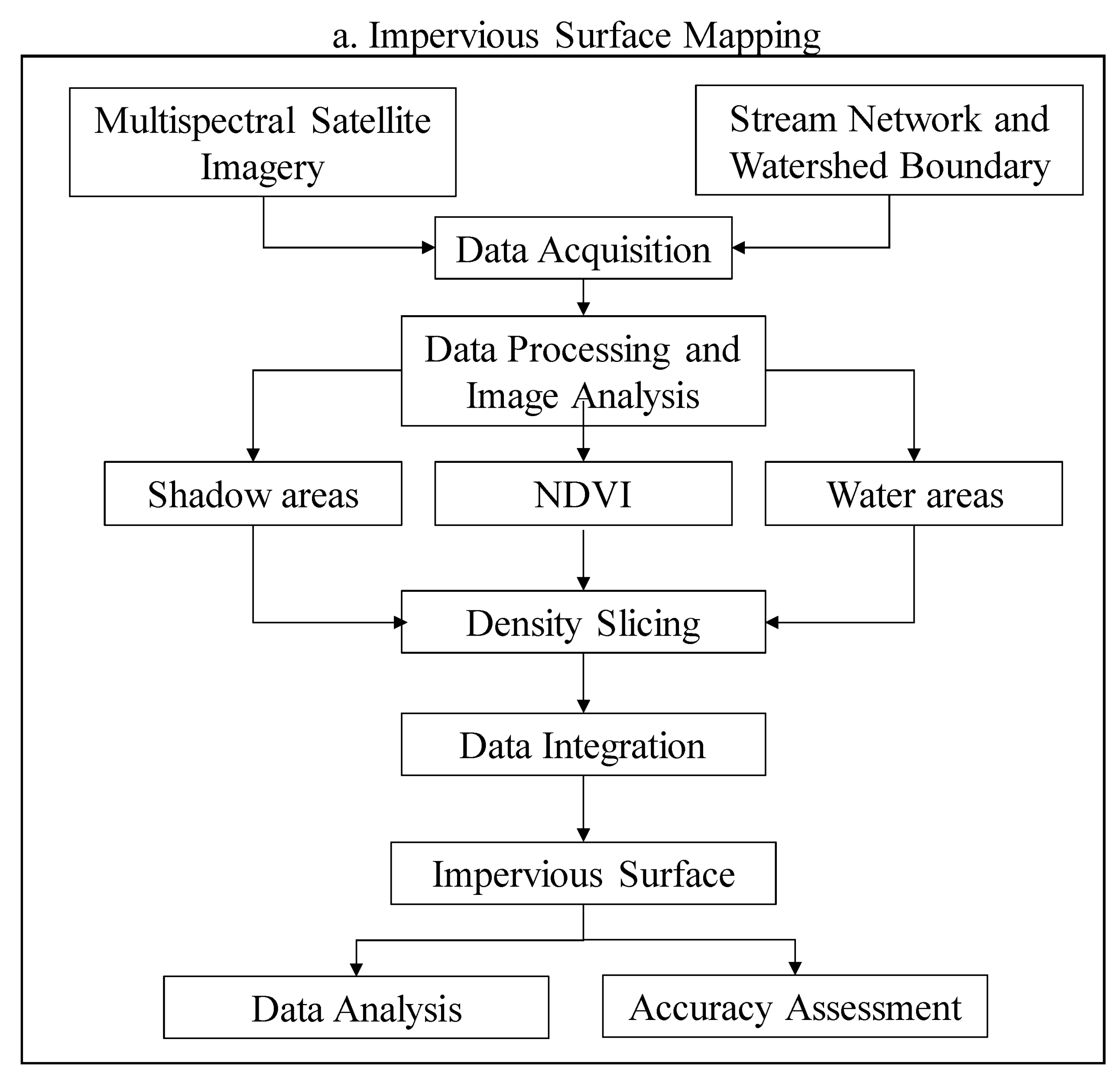
A pair of satellite imagery acquired by NASA’s Landsat missions was used in this study. The first scene was acquired by Landsat 5 Thematic Mapper (TM) on 24 January 1986 and was used to study the land use and land cover (LULC) of 1986. The second scene was acquired by Landsat 8 Operational Land Imager (OLI) on 26 November 2016 and was used to study the LULC of 2016. The processing and analysis of the imagery and the overall methodological scheme are explained in Figure 2.

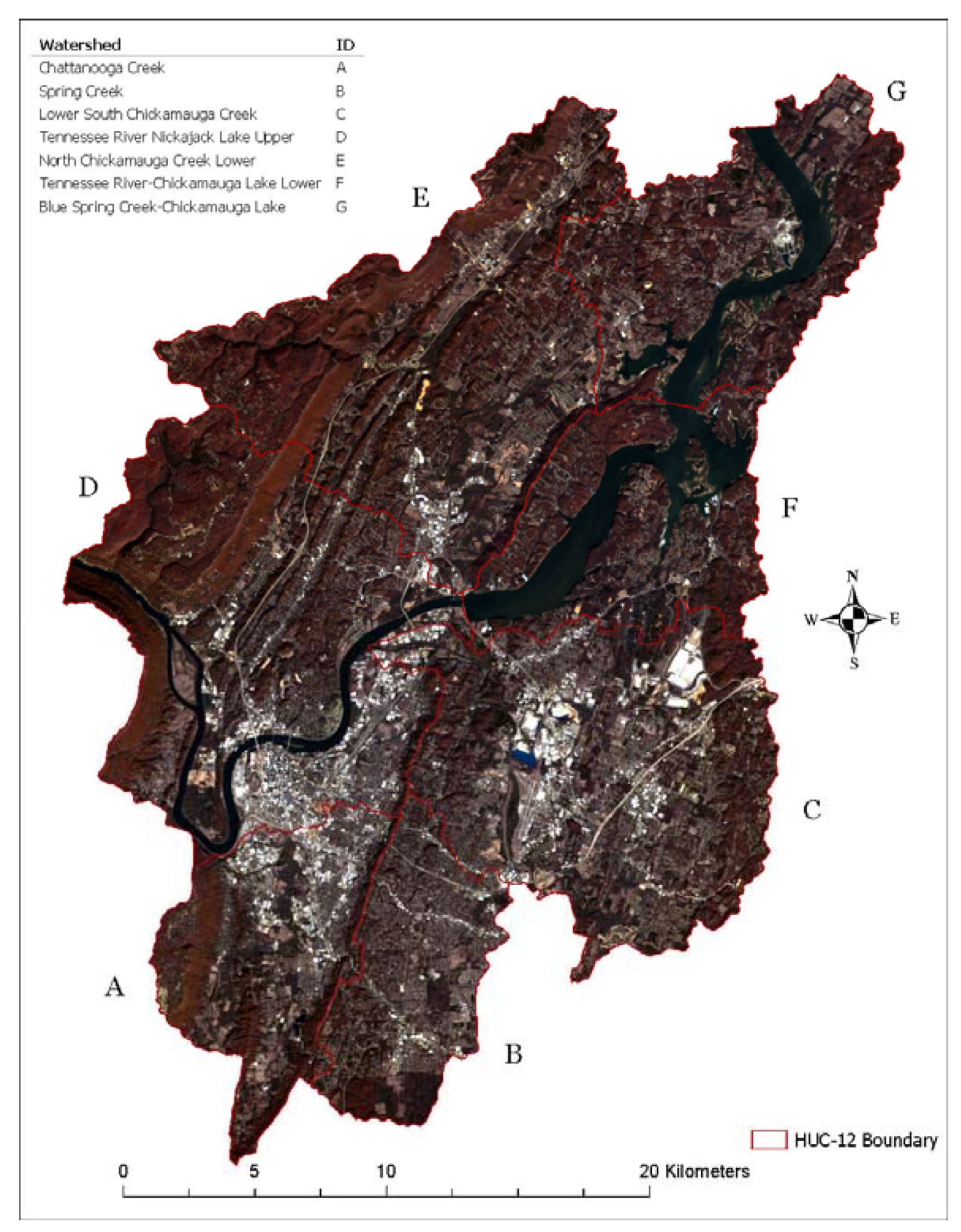
Both satellite images in the Red Green Blue (RGB) and Near Infra-Red (NIR) spectrums have a spatial resolution of 30 m. The true color displays of Landsat 5 TM and Landsat 8 OLI images for the study site can be seen in Figure 3 and Figure 4, respectively. Since the two images were collected by different Landsat sensors with a significant temporal gap between acquisitions, atmospheric correction was needed to convert both images into the same radiometric scale [138]. The conversion of the image values to represent the surface reflectance requires the correction of atmospheric effects on exiting electromagnetic radiation, which is an important image pre-processing step [139,140]. The Landsat 5 TM scene reflectance values were generated using NASA’s Landsat Ecosystem Disturbance Adaptive Processing System (LEDAPS) software [141]. For the Landsat 8 OLI scene, NASA’s Landsat Surface Reflectance Code (LaSRC) was used to generate the values [142].

A one-meter resolution multispectral aerial photograph acquired by the United States National Agricultural Imagery Program (NAIP) in 2014 over the study site was obtained for the accuracy assessment part of the study. The obtained NAIP imagery included both RGB and NIR bands. The Tennessee county and state boundary data were collected from the Tennessee State government GIS data server and the U.S. Census Bureau’s data server, respectively. The watershed data were collected from the USGS National Hydrography Dataset Plus (NHDplus) and the City of Chattanooga Water Quality Program. The stream location data were collected from NHDplus and the City of Chattanooga GIS Office.

2.3. Mapping Impervious Surfaces

The satellite data used for this research were pre-processed including geo-rectification and restoration [143]. Once the Landsat data and NAIP imagery were collected, necessary bands for each dataset were masked to the study site and stacked to create the Red Green Blue (RGB) and Near Infra-red (NIR) composite imagery. The model designed for mapping impervious surfaces (IS) is based on the application of Normalized Difference Vegetation Index (NDVI) due to the breaks in values for different land covers, which can be used to isolate impervious surface (IS) areas. To assist in land cover isolation, the NIR band was used to separately classify water resources, and the green band for shadows in both images. The model developed for detecting and mapping impervious surfaces is represented by Equation (1).

$$I{S}_{Data}=I{S}_{NDVI}-Shado{w}_{Green}-Wate{r}_{NIR}$$

(1)

where IS_NDVI represents a NDVI image that has been classified into IS and vegetated areas, Shadow_Green represents shadows (detected by the green band of a Landsat sensor), and Water_NIR represents surface waterbodies (detected by the NIR band of a Landsat sensor).

All image processing and analyses were conducted using ArcGIS Pro GIS software [144]. The statistical tests applied were conducted in the Jupyter Notebook environment using Python scripting language [145].

2.4. Normalized Difference Vegetation Index (NDVI)

The primary component of the developed IS mapping model is NDVI. This index, seen in Equation (2), uses the NIR and red (R) portions of the EMS.

$$\mathrm{NDVI}=\frac{\left({\rho }_{NIR} - {\rho }_R\right)}{\left({\rho }_{NIR }+ {\rho }_R\right)}$$

(2)

where ρ_NIR is the surface reflectance value of NIR and ρ_R is the surface reflectance value of R.

The Normalized Difference Vegetation Index was originally developed to map green vegetation, which has a sharp contrast in the amount of absorption of red wavelengths compared to near infrared [62]. Green vegetation has a high absorption of light in the red portion of the Electromagnetic Spectrum (EMS) while reflecting a significant portion of the NIR portion; this response is driven primarily by the vegetation’s photosynthetic activity [146]. This difference in EMS absorption causes areas of healthy, green vegetation to have large, positive values from NDVI. This index can also be used to map other non-vegetated land covers, primarily water and IS, due to each land cover’s distinct interactions with red and NIR wavelengths [55]. Where IS have close to equal reflection of both red and NIR light, they generate NDVI values close to 0 [146]. Negative NDVI values indicate non-vegetated areas often consisting of water [146]. A NDVI was generated for each image, to separate the vegetated and non-vegetated areas [64]. This concept of mapping vegetation to subsequently extract exposed IS has been previously established as an alternative method for estimating IS [147].

The Landsat 5 TM NDVI equation can be seen in Equation (3) and the Landsat 8 OLI NDVI equation can be seen in Equation (4).

$$\mathrm{Landsat}5\mathrm{TM}\mathrm{NDVI}=\frac{\left({\rho }_{B4} - {\rho }_{B3}\right)}{\left({\rho }_{B4 }+ {\rho }_{B3}\right)}$$

(3)

where ρ_B4 and ρ_B3 represent the reflectance values of NIR and R, respectively.

$$\mathrm{Landsat}8\mathrm{OLI}\mathrm{NDVI}=\frac{\left({\rho }_{B5} - {\rho }_{B4}\right)}{\left({\rho }_{B5 }+ {\rho }_{B4}\right)}$$

(4)

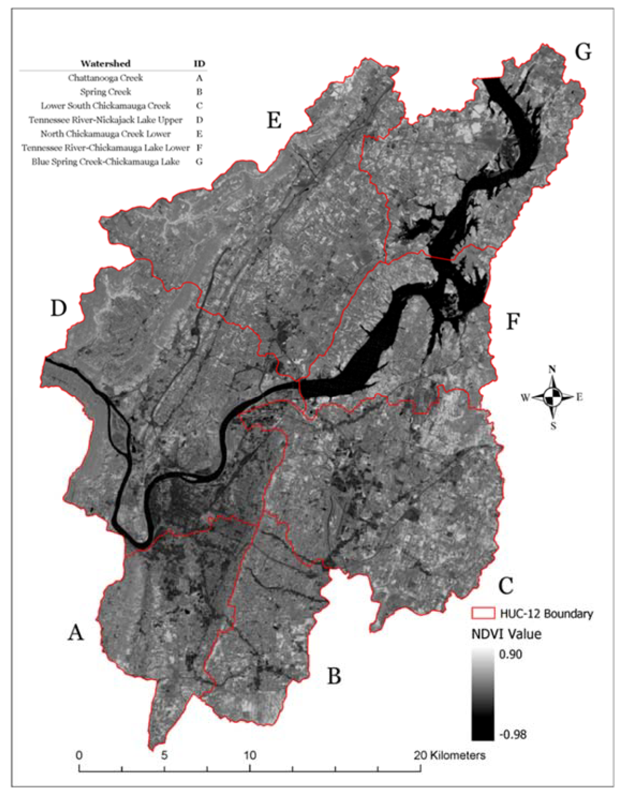
where ρ_B5 and ρ_B4 represent the reflectance values of NIR and R, respectively. Figure 5 shows the NDVI image generated for 1986 and Figure 6 shows the NDVI image generated for 2016.

2.5. Image Classification

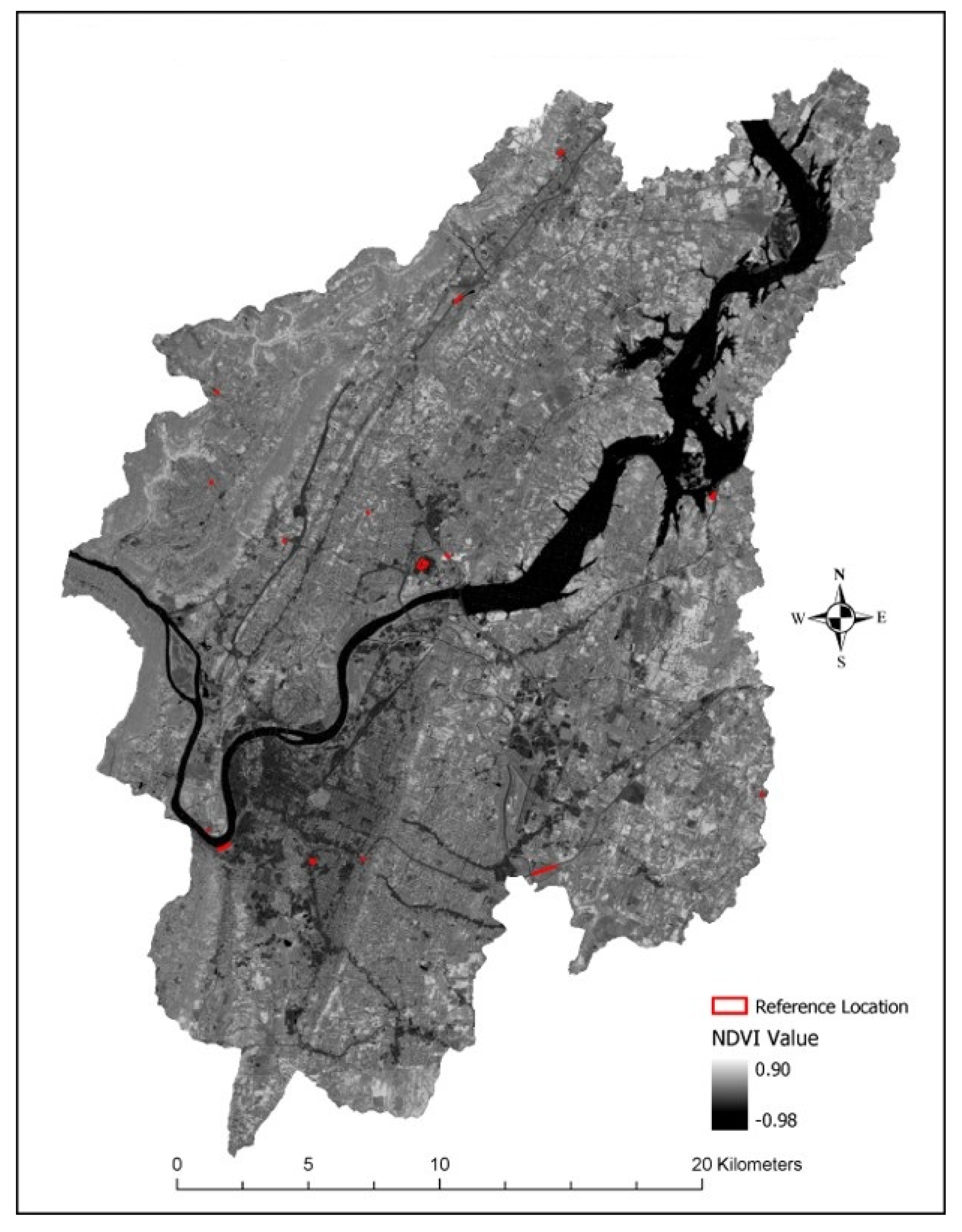
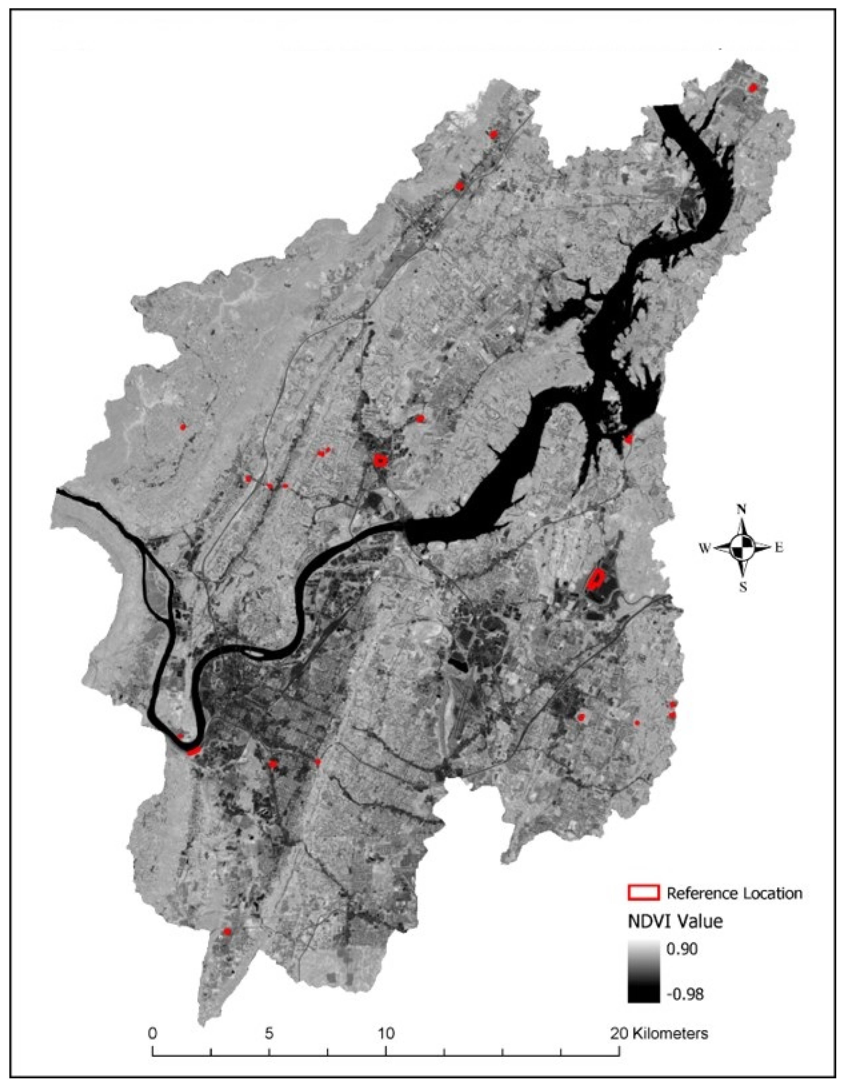
To classify desired land covers, density slicing classification was performed. This classification method requires the researcher to determine the spectral response range of desired variables from a single layer image. This is conducted by an initial manual or statistical-based classification of an image based on the distribution of the pixel values. Then, continued re-classification is conducted by adjusting pixel value threshold until the desired land cover has been effectively isolated. Reclassification and verification can be improved using reference location data, which can be colored imagery and/or pre-labeled reference areas. Density slicing technique was applied on the generated Landsat 5 and Landsat 8 Normalized Difference Vegetation Index (NDVI) images to classify them into impervious surface (IS) and vegetated areas. Density slicing was also used to categorize waterbodies using the NIR band and shadows with the green band for each date. To assist in classification for each date, the true color Landsat image was used as a visual reference for each date. Reference polygons were used to assist in determining IS land cover threshold values for both 1986 and 2016. Figure 7 and Figure 8 show the density slicing reference locations used. Figure 9 shows examples of reference polygons for both 1986 and 2016 with the NDVI image and true color image for comparison. During density slicing, repeated inspection of these anchor points were conducted to gauge the effectiveness of the used pixel threshold values.

Table 2. The threshold values for density slicing classification for the 1986 Landsat 5 Thematic Mapper (TM) and 2016 Landsat 8 Operational Land Imager (OLI) images.

Land Cover Type	Year	Data	Threshold Value
Shadows	1986	Green Band	(142, 330)
	2016	Green Band	(33, 225)
Vegetation	1986	NDVI	(0.255873, 0.790147)
	2016	NDVI	(0.385, 0.902)
Water	1986	NIR Band	(38, 350)
	2016	NIR Band	(4, 190)
IS	1986	NDVI	(−0.02992, 0.255873)
	2016	NDVI	(−0.09, 0.385)

gives the threshold values determined for each class.

2.6. Data Integration

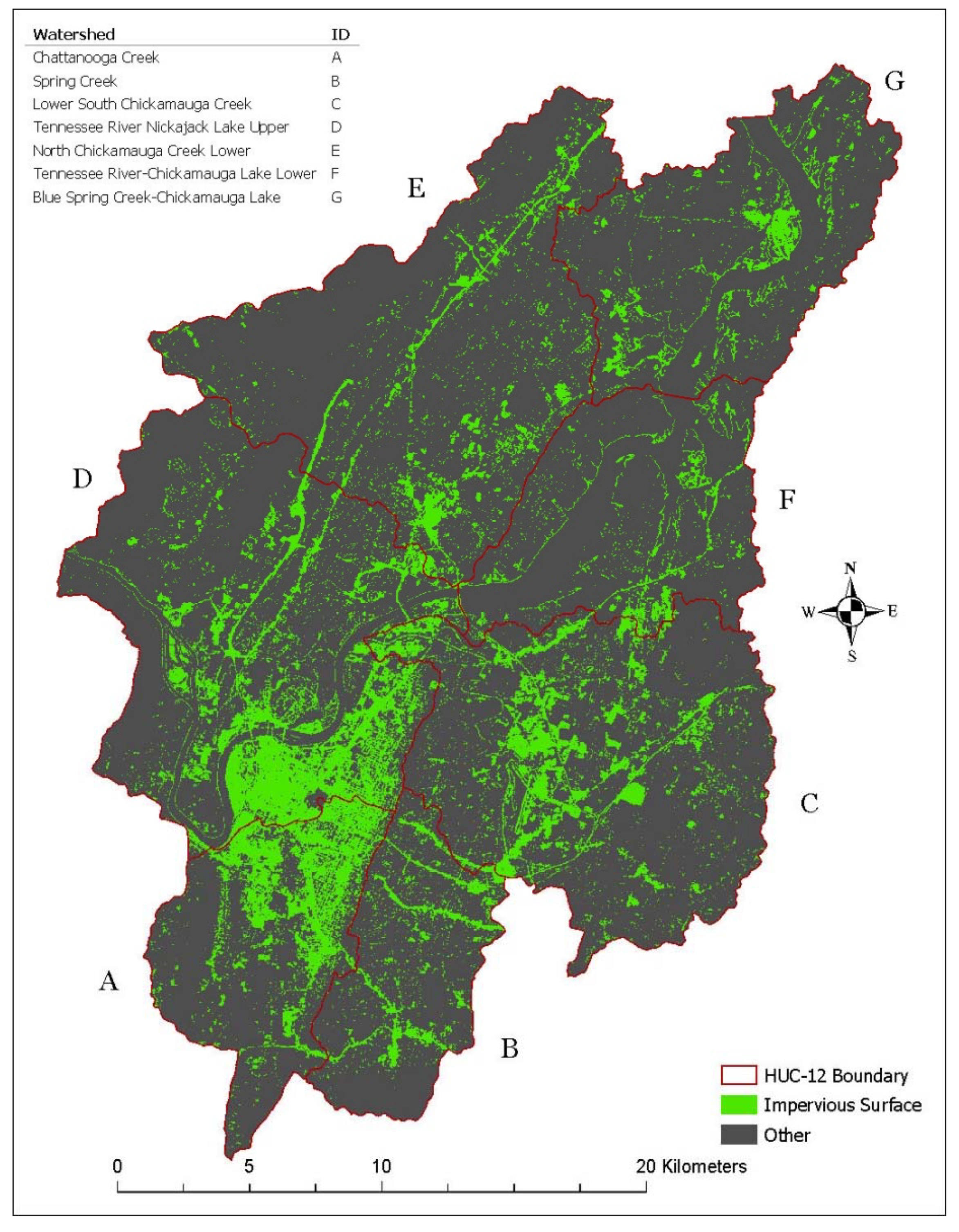
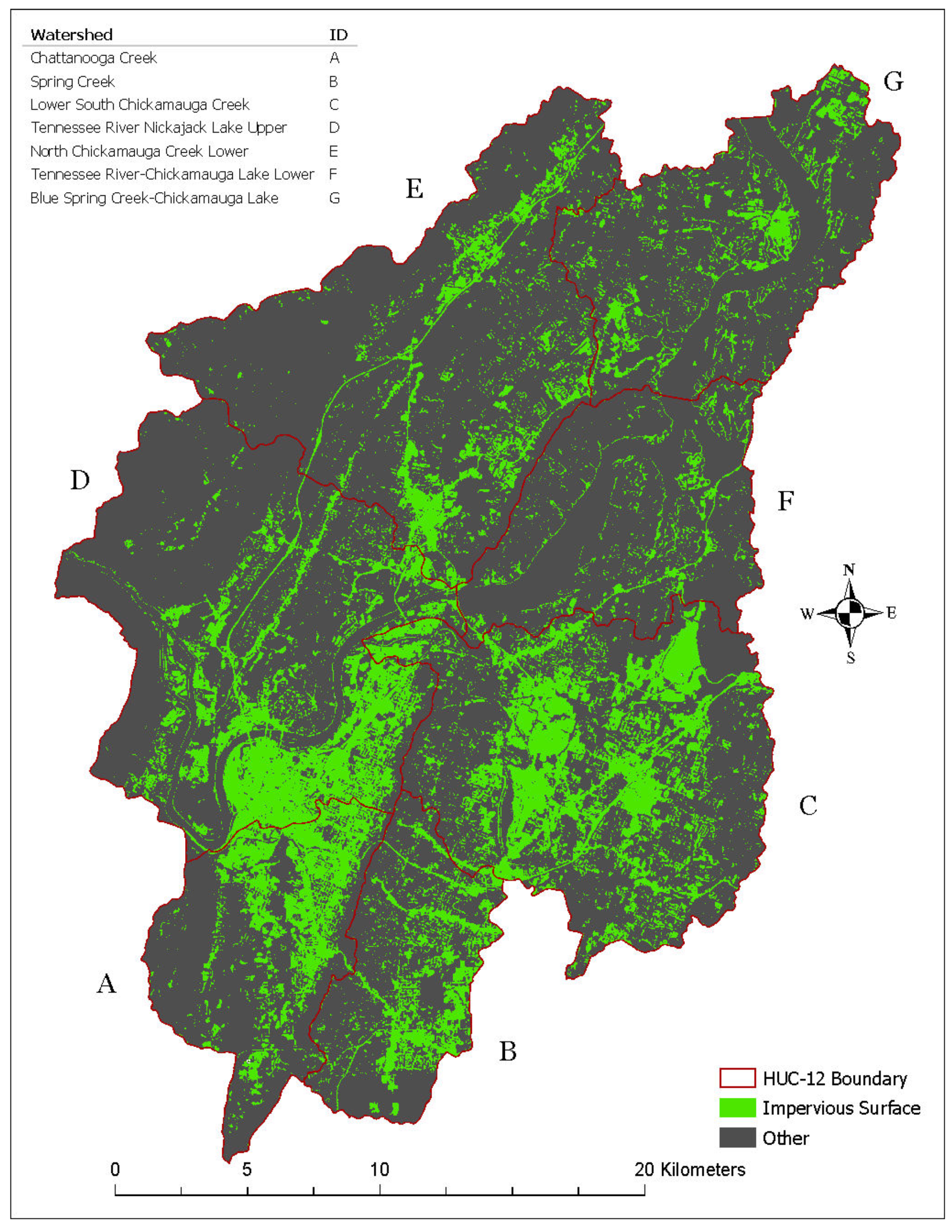
Using raster algebra, the final IS dataset for each date was created by combining the classified NDVI, green band and Near Infra-Red (NIR) band datasets using a nested conditional statement executed with the ArcGIS raster calculator tool. The conditional statement isolated each desired land covers from each dataset and returned a single dataset containing all the classified classes. The resulting datasets were then reclassified into two classes: (1) impervious surfaces and (2) pervious and other surfaces. This reclassified thematic image represents the final IS dataset. The IS dataset is seen in Figure 10 and Figure 11 for 1986 and 2016, respectively.

2.7. Accuracy Assessment

The accuracy assessments of the resulting impervious surface (IS) datasets were conducted using two different techniques: (1) Zonal Statistics and (2) Kappa Statistics.

2.7.1. Zonal Statistics

Zonal statistics was used for the accuracy assessment of the (IS) models for both 2016 and 1986. For the 2016 model, this was conducted by digitizing 140 randomly located reference IS areas within the study site. Figure 12 shows the locations for the 2016 reference IS areas. Each HUC-12 watershed contains 20 of the digitized reference polygons. Every reference IS polygon covers an area equal to 15 m². The NAIP dataset was used as the source of these reference IS polygons. A majority count zonal statistic was applied to the digitized reference polygons overlaying the impervious dataset. This was conducted to determine if the majority of the classified pixels covered by the reference polygons were impervious or pervious. Due to resource constraints, it was not possible to obtain high resolution aerial photography to generate reference polygons to evaluate the 1986 dataset. In this case, a true color Landsat 5 TM image was used to obtain the 140 reference polygons. The reference polygons digitized using the NAIP data that contained 100% IS on the Landsat 5 TM image were used for the accuracy assessment. Only 60 polygons digitized with NAIP imagery represented 100% IS cover in 1986. These polygons were then used to assess the accuracy of the 1986 IS dataset following the methods used for the 2016 dataset.

2.7.2. Kappa Statistics

A confusion matrix and Cohen’s Kappa-coefficient (k) were calculated for each date. The Kappa statistic has been shown to be an effective measure of a classification model in remote sensing and other scientific fields, due to its ability to evaluate the interclassifier agreement and remove the bias [148,149,150]. Kappa statistics evaluated the performance of the IS classification models by calculating the User’s accuracy (Type I error or false positive) and Producer’s accuracy (Type II error or false negative) for each class, the proportion of pixels correctly classified (PCC), and Kappa-coefficient of agreement. The Producer’s accuracy reports the error of omission created by the model, quantifying the amount of each class that have not been correctly classified. The equation for the Producer’s accuracy is shown by Equation (5).

$$\mathrm{Producer}\text{’}\mathrm{s}\mathrm{Accuracy}=\frac{C_T}{C_T+O_C}$$

(5)

where C_T is the amount of a class C that is correctly classified, and O_C is the sum of other classes that were classified as C.

The User’s accuracy reports the error of commission which is the amount of other classes that have been classified incorrectly. The equation for the User’s accuracy is shown by Equation (6).

$$\mathrm{User}\text{’}\mathrm{s}\mathrm{Accuracy}=\frac{C_T}{C_T+C_E}$$

(6)

where C_E is the sum of the class that are incorrectly classified.

The proportion of pixels correctly classified (PCC) is calculated by dividing the total number of correctly classified pixels by the total number of pixels classified. The equation for calculating overall accuracy of a classification model is shown as Equation (7).

$$\mathrm{PCC}=\frac{n_T}{n}$$

(7)

where n_T is the sum of correctly classified subjects and n is total subject sample size.

The Kappa-coefficient of agreement (k) describes the accuracy of the classification model compared to random classification on the assumption that some of the pixels could have been classified correctly by chance. The equation for calculating the Kappa-coefficient is shown by Equation (8).

$$K=\frac{P_O-P_E}{1-P_E}$$

(8)

where P_O is the observed agreement of classification, P_E is the chance agreement of classification and 1 represents maximum agreement. To calculate P_O and P_E Equations (9) and (10) were used.

$$P_O=\frac{O_D}{n}$$

(9)

$$P_E=\frac{E_D}{n}$$

(10)

where O_D is the sum of the observed frequencies along the diagonal in the confusion matrix, E_D is the sum of expected frequencies along the horizontal and n is the total number of subjects.

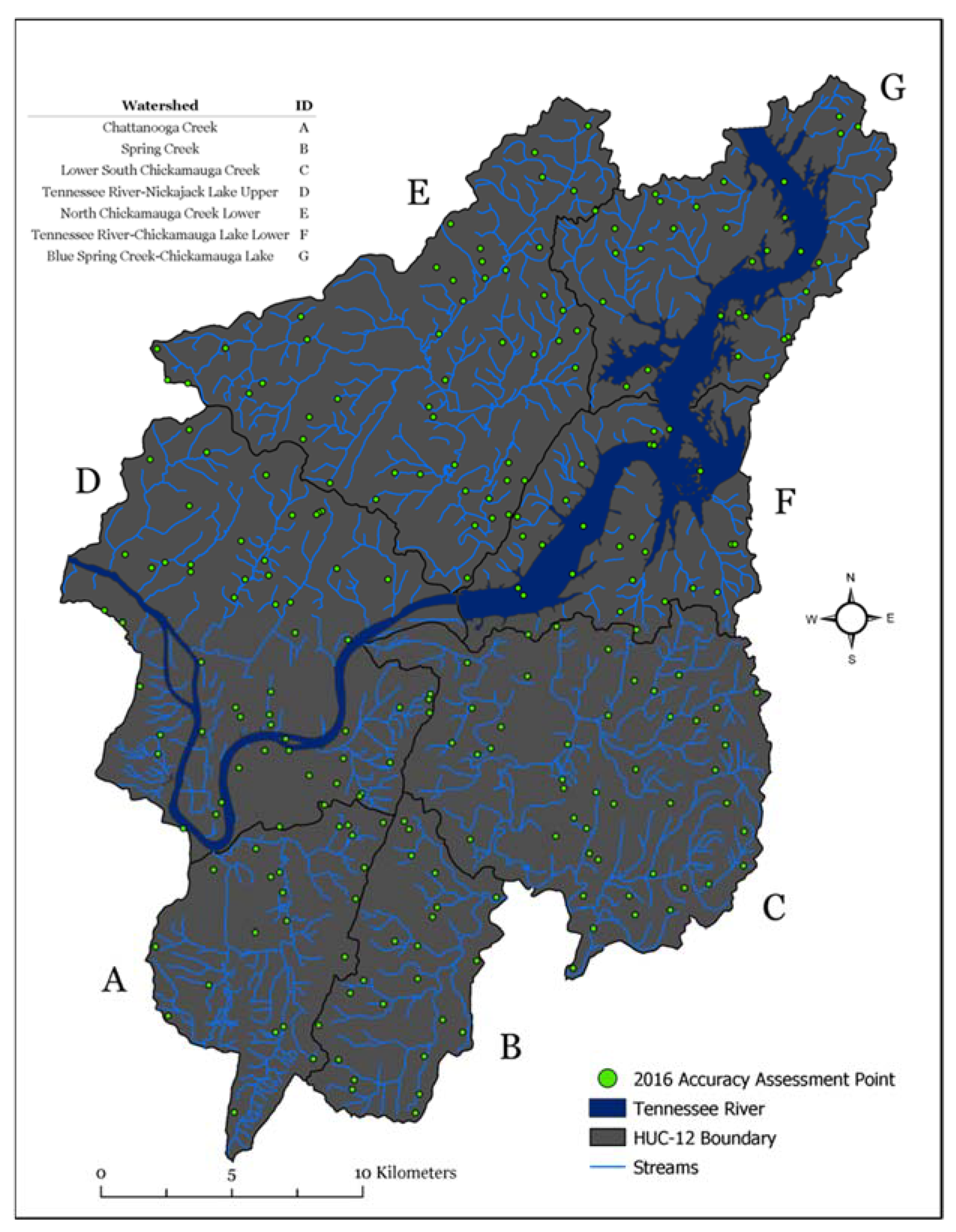
To generate the confusion matrix, 250 randomly stratified accuracy assessment points were generated for each date. These points were validated using the relevant Landsat image. For 2016, the NAIP imagery from 2014 was also used in this regard. The locations of the assessment points of the confusion matrix generation can be seen in Figure 13 and Figure 14 for 1986 and 2016, respectively.

2.8. Water Resource Proximity Analysis

To understand the spatial relationship of the impervious surface (IS) growth regarding water resources within the study site, IS change per HUC-12 watershed (and stream riparian areas) was measured. The obtained IS datasets were clipped by each of the selected HUC-12 watershed boundaries for quantification of the IS change in each HUC-12 watershed. IS area was calculated by multiplying the total number of IS pixels with the area of a single pixel (30 m × 30 m). Finally, the obtained values were converted to km².

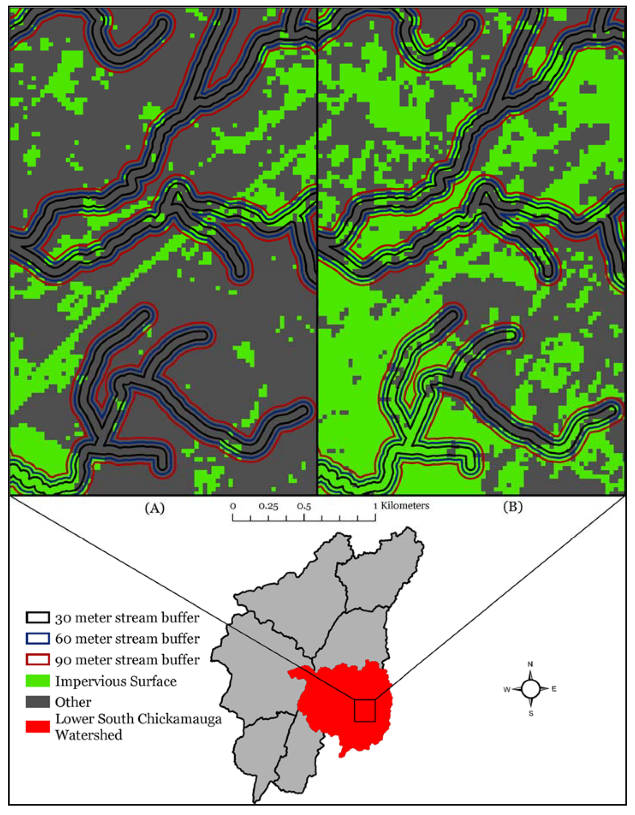
For the stream analyses, streams within the study site were obtained from the NHDplus dataset and combined with auxiliary data from the City of Chattanooga Water Quality Program. The first stream analysis was performed by creating buffer distances of 30 m, 60 m, and 90 m on both sides of the selected streams. A map showing the stream buffers generated can be seen in Figure 15. After the buffer polygons were generated, they were clipped by each of the HUC-12 watersheds to create separate watershed riparian buffer boundaries for each watershed within the study site. The obtained polygon features were then used to extract impervious surface (IS) pixels from both IS datasets. IS area was then calculated in km² for each of the buffer features using the quantity of IS pixels and the area coverage for a single pixel. The proximity analysis was conducted in ESRI’s ArcGIS Pro GIS environment and the bar charts for reporting the results were generated using the Python scripting language in the Jupyter Notebook environment.

2.9. Assessing Stream Risk

To assess the probability of stream impairment due to impervious surface (IS) change, a model was developed to independently assess streams for their potential risks. The model evaluates stream segments to provide further detail regarding sections of streams that may have higher risk due to new or existing developments. More specifically, the model accounts for both the quantity of changes in IS and the proximity of those changes to the stream segments evaluated. Percent imperviousness was calculated for each buffered polygon and was incorporated with the model. The risk assessment was conducted in ESRI’s ArcGIS Pro GIS environment. The bar charts were generated using the Python scripting language in the Jupyter Notebook environment [145].

2.9.1. Stream Segmentation

The segmentation of streams was done by generating points at every 90 m along the stream with points also placed at the ends of the stream and at the intersection of stream branches. These points were then used to splice the original stream datasets and to act as end points for new, unique stream segments. A total of 12,910 stream segments were generated within the study site. Some segments were shorter than 90 m due to stream branching and/or small stream segment lengths.

2.9.2. Riparian Zone Generation

Both IS datasets were converted from pixels to points, which represented the centers of the original pixels. The obtained IS point datasets were used to perform a spatial analysis technique called ‘spatial join’. Spatial join summarizes and joins the attributes of features that meet a pre-determined spatial criterion, to be performed for points within 30 m, 60 m, and 90 m of each stream segment. This zone of influence considers all land cover within these distances from any point along the segment, including the start and end points. The attributes of each IS dataset were then summarized per segment of the stream in the zone.

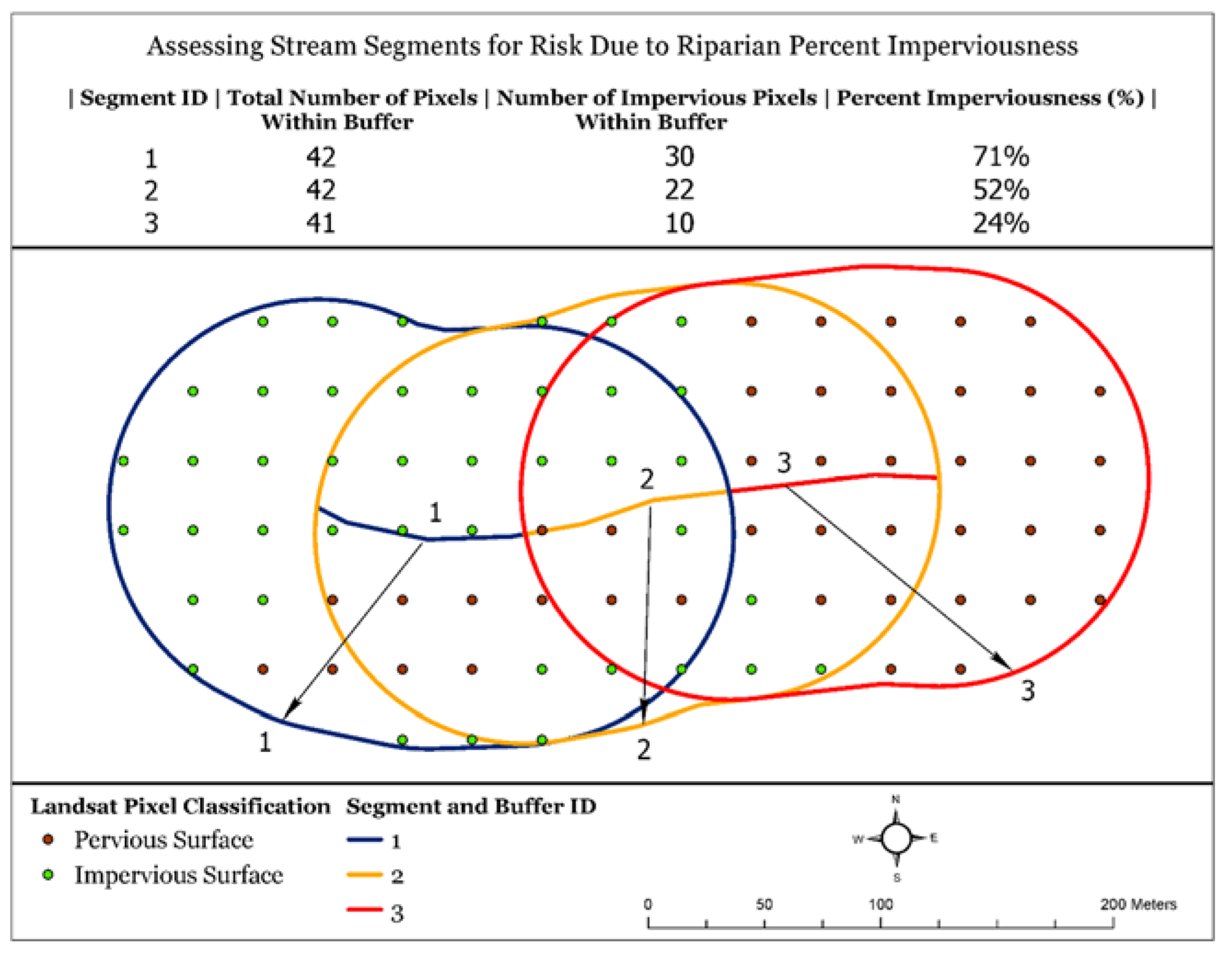
These results allowed for quantifying and locating the IS growth around each stream segment within the study site. Quantification of the amount of IS development were normalized using the number of points within each zone. The normalization by area generated a percent imperviousness value per zone of influence surrounding each stream segment. By subtracting the 30 m zone results from the 60 m zone results and the 60 m zone from the 90 m zone, the area with each segment was partitioned into three evenly spaced, 30m wide riparian zones. This relationship between spatial join buffer sizes and riparian zone creation can be seen in

Table 3. Riparian buffer interval distance from streams and equivalent stream buffer variables.

Interval Distance Range from Stream (m)
	0–30	30–60	60–90
Variable	X1	X2	X3
Proximity Weight	3	2	1
Buffer Distance Range from Stream (m)
	0–30	0–60	0–90
Variable	X	Y	Z
Interval Equivalent	X1	X1 + X2	X1 + X2 + X3

. Figure 16 demonstrates how each segment considers the points within the zone of influence and how the percent imperviousness for the riparian area is generated. The model is based on the understandings that riparian areas up to 150 m from the stream can have significant impacts of stream water quality [151]. The proximity of the development is considered to have a stronger impact on the stream than the development which occurred father away [152,153].

2.9.3. Relating IS Development Proximity and Quantity to Risk

A linear weighted model was then developed and applied to each segment to calculate the probability of surface water impairment due to the distance and magnitude of percent imperviousness in each riparian zone. This model can be seen in Equation (10).

$$\mathrm{IS}\mathrm{proximity}\mathrm{risk}\mathrm{model}=\left(W_3\times X_1\right)+\left(W_2\times X_2\right)+\left(W_1\times X_3\right)$$

(11)

where X₁, X₂, and X₃, represent the percent imperviousness (normalized) within the three separate 30 m riparian zones, and W₁, W₂, and W₃, represent the IS-stream influence weight. The values for the IS-stream influence weight are shown as the subscript numeral. The weights were incorporated arbitrarily using the values of 1 to 3, where the value of 3 represents the most influential, 2 represents the moderately influential and 1 represents the least influential. These values reflect that usually the influence of the growth of IS on the stream will have more influence from the nearby development. The output of this model indicates the portions of the streams, within the study site, that have an increased probability of being impaired due to the surrounding IS development.

3. Results and Analysis

3.1. Impervious Surface (IS) Mapping

According to the results of zonal statistics, the accuracy for the IS classification of 1986 was 88.3%. That is, 53 of the 60 reference polygons were correctly classified as IS. The accuracy for the IS classification of 2016 was 90%. That is, 126 of the 140 reference polygons were correctly classified as IS. The confusion matrix prepared for 1986 is shown in

Table 4. Confusion matrix for the 1986 Landsat 5 TM IS classification.

Classification	Other	Impervious	Total	User’s Accuracy	Kappa (k)
Other	198	12	210	94.3%
Impervious	13	27	40	67.5%.
Total	211	39	250
Producer’s Accuracy	93.8%	69.2%		90.0%
Kappa (k)					0.624

. The overall accuracy reported by the confusion matrix for 1986 is 90.0%. The Kappa-coefficient calculated is 0.624, showing that the model for 1986 classified 62.4% better than a random classification of the data. The confusion matrix prepared for 2016 is shown in

Table 5. Confusion matrix for the 2016 Landsat 8 OLI IS classification accuracy.

Classification	Other	Impervious	Total	User’s Accuracy	Kappa (k)
Other	178	16	194	91.7%
Impervious	22	34	56	60.7%
Total	200	50	250
Producer’s Accuracy	89%	68%		84.8%
Kappa (k)					0.545

. The overall accuracy reported by the confusion matrix for 2016 is 84.8%. The Kappa-coefficient calculated is 0.545 showing that the model for 2016 performed 54.5% better than a random classification. The values of Kappa statistic ranging from 0.41 to 0.6, and from 0.61 to 0.80 can be interpreted to represent moderate and substantial agreement for a classification, respectively [154]. According to this interpretation, the accuracy of the classification model for 1986 dataset can be described as substantial. Similarly, on the other hand, the accuracy of the classification model for 2016 dataset can be described as moderate.

The total HUC-12 IS area calculations performed on this study’s model show that there has been a significant growth in the study site as shown in Figure 17 and described in

Table 6. Quantitative estimation of the IS areas mapped for the seven HUC-12 watersheds in Hamilton County as observed on 24 January 1986 and 26 November 2016.

Impervious Surface (IS) Area in Square Kilometers and Percentage
HUC Watershed	1986	2016	Percent Increase
Chattanooga Creek	20.12	20.11	−0.1%
Spring Creek	7.42	14.24	91.9%
Tennessee River - Nickajack Lake Upper	37.93	40.31	6.3%
Tennessee River Chickamauga Lake Lower	9.26	13.91	50.2%
Lower South Chickamauga Creek	24.23	48.48	100.8%
North Chickamauga Creek lower	14.63	20.85	42.5%
Blue Spring Creek - Chickamauga Lake	6.73	7.54	12.0%

. The net growth within the study site was 45.12 km². This growth was not spatially equal in its distribution and occurred heavily in the Lower South Chickamauga Creek watershed with an increase of 24.3 km² of IS. The Lower South Chickamauga Creek watershed had the largest percent increase in impervious development with a change from 24.2 to 48.5 km², equaling slightly more than a 100% increase in impervious area. All but the Chattanooga Creek watershed showed an increase in IS with development being less than 10 km² in each area. Finally, the Chattanooga Creek watershed had a small decrease in IS area, decreasing by 0.01 km².

3.2. Water Resource Proximity Analysis

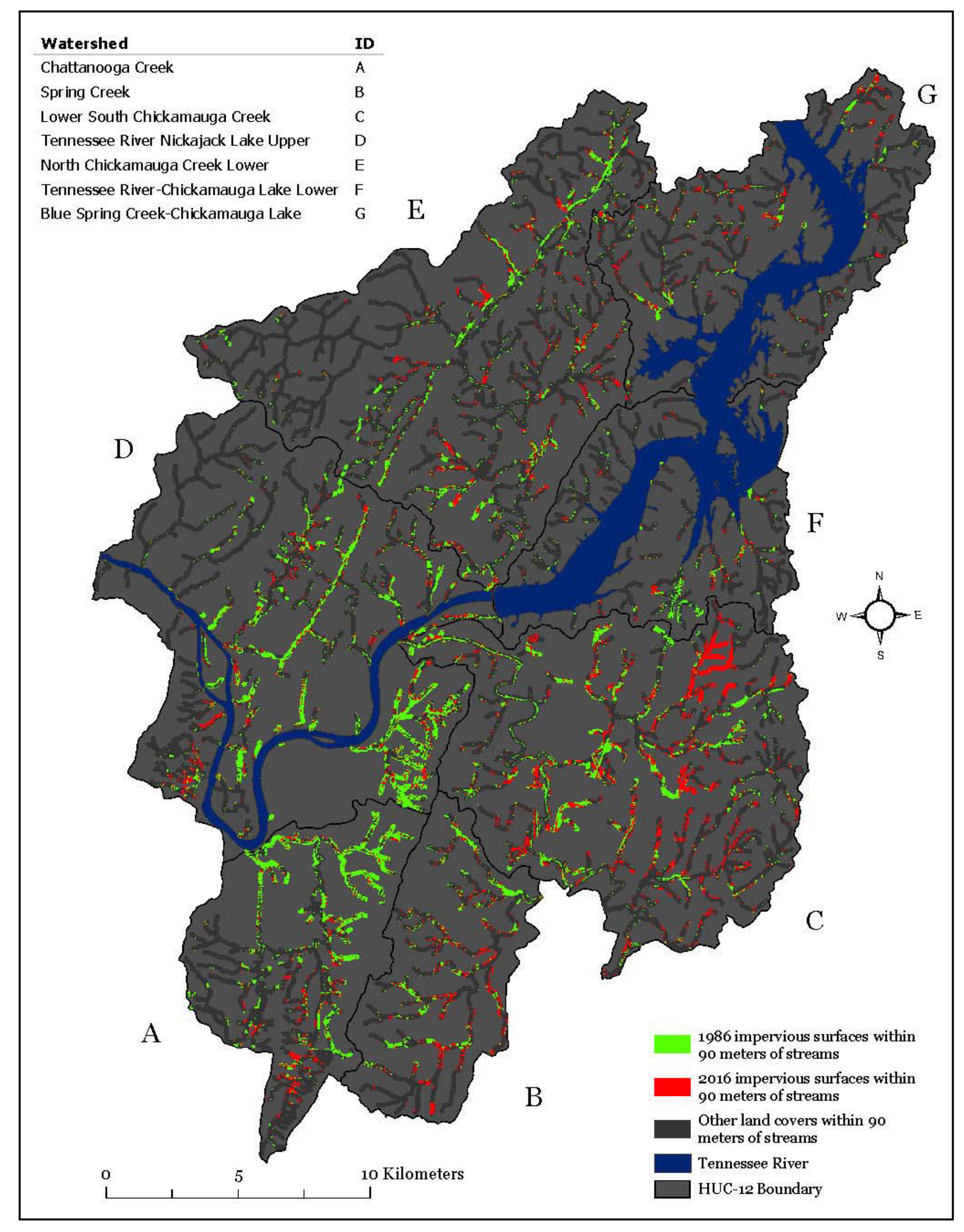
The impervious surface (IS) growth estimated shows that there has been significant IS growth near selected streams in the study site. The results of this analysis can be seen in Figure 18 and summarized in

Table 7. IS growth within buffers of streams within the study site for 1986 and 2016.

Impervious Surface (IS) Area in Square Kilometers within Stream Riparian Zones
Zones	30 m			60 m			90 m
Watershed ID	1986	2016	% Change	1986	2016	% Change	1986	2016	% Change
A	1.49	1.32	−11.5	3.18	3.07	−3.5	4.89	4.91	0.4
B	0.47	0.89	89.4	1.00	1.90	90.0	1.57	2.98	89.8
C	2.59	2.74	5.7	5.42	5.72	5.5	8.07	8.84	9.5
D	0.40	0.70	75	0.77	1.41	83.1	1.13	2.14	89.4
E	2.16	3.52	63	3.99	7.28	82.4	5.71	11.34	98.6
F	1.54	1.52	−1.3	2.99	3.39	13.4	4.42	5.46	23.5
G	0.27	0.28	3.7	0.55	0.60	9.1	0.91	1.00	9.9

Watershed ID key: Chattanooga Creek (A), Spring Creek (B), Lower South Chickamauga Creek (C), Tennessee River-Nickajack Lake Upper (D), North Chickamauga Creek Lower (E), Tennessee River-Chickamauga Lake Lower (F), Blue Spring Creek-Chickamauga Lake (G).

. In 1986, IS cover accounted for 14.9% of the total area within 30 m of streams, increased to 18.1% by 2016. Compared to the change within 90 m of streams, where in 1986, IS cover occupied 15.2%, increased to 20.9% by 2016. The net growth of IS within 90 m of streams was 9.96 km². The total increase of IS within the first 30 m was 2.04 km², with an increase of 3.43 km² between 30 m and 60 m, and 4.49 km² between 60 m and 90 m of streams. The average change in IS area for the 30 m, 60 m and 90 m buffers in each HUC-12 watershed was 0.29, 0.49, and 0.64 km², respectively. IS development within 90 m of streams accounted for 22% of the total IS development detected. Changes in IS extent within the stream riparian areas within the study site are shown in Figure 18, which shows the coverage of IS in riparian areas in green and the added extent in 2016 in red.

The Lower North Chickamauga Creek watershed experienced a decrease of 0.024 km² of IS within 30 m of streams but reported large increases in IS for the 60 m and 90 m buffers. The Chattanooga Creek watershed experienced a decrease in IS within 30 m and 60 m of streams but did experience a small increase within 90 m. There was growth for the remaining five watersheds at each buffer distance with similar trends found in the total HUC-12 IS area analysis. The Lower South Chickamauga Creek watershed showed the largest growth of IS development in each of the three distance zones. It experienced an increase of 1.35 km² within 30 m of streams, 3.29 km² within 60 m, and 5.63 km² within 90 m. This equated to being 66.3%, 60.1% and 56.4% of the total IS development regarding each buffer distance. A portion of the Lower South Chickamauga Creek IS change in relation to stream buffers is shown in Figure 19.

3.3. Riparian Development and Risk Analysis

3.3.1. Riparian Percent Imperviousness

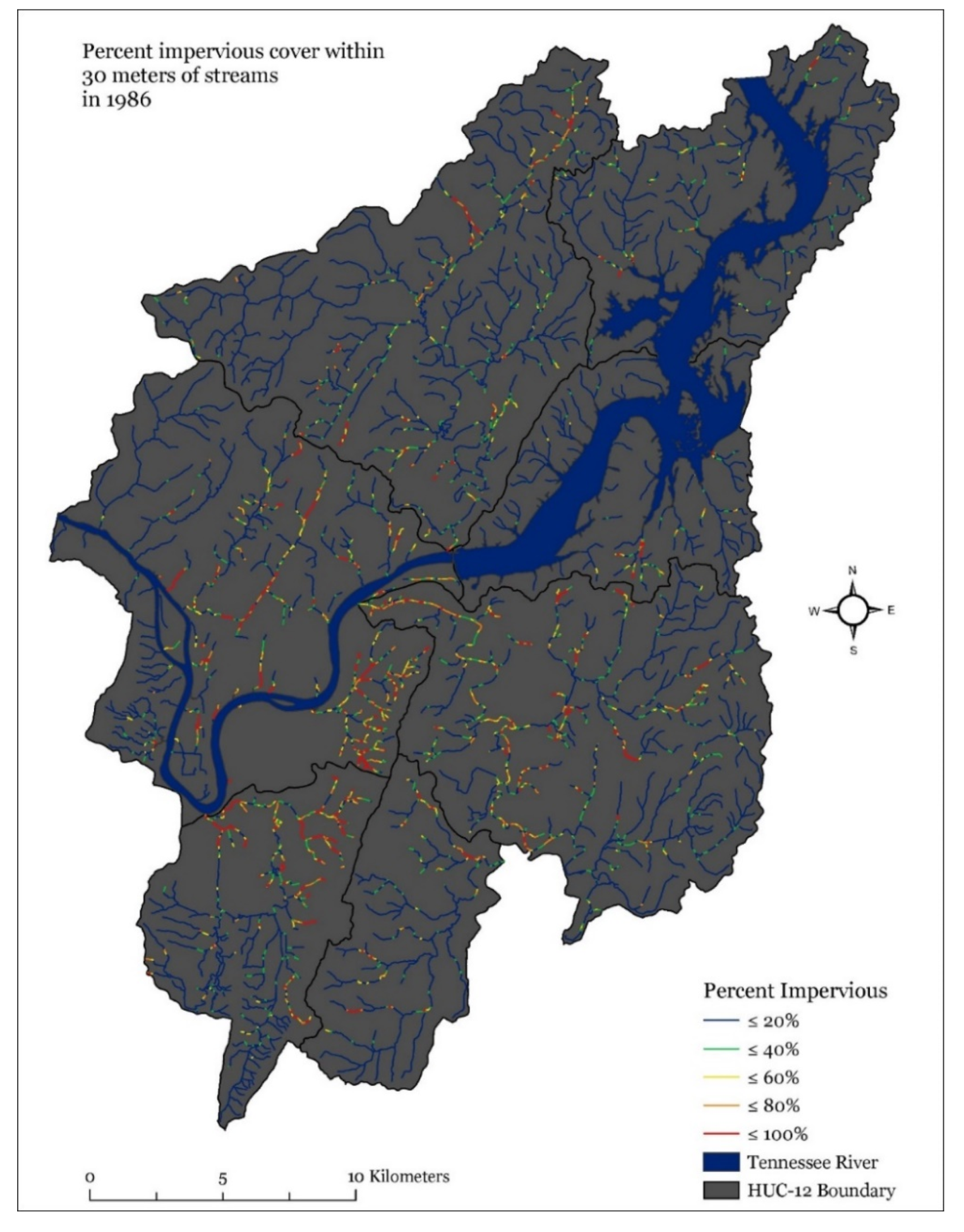
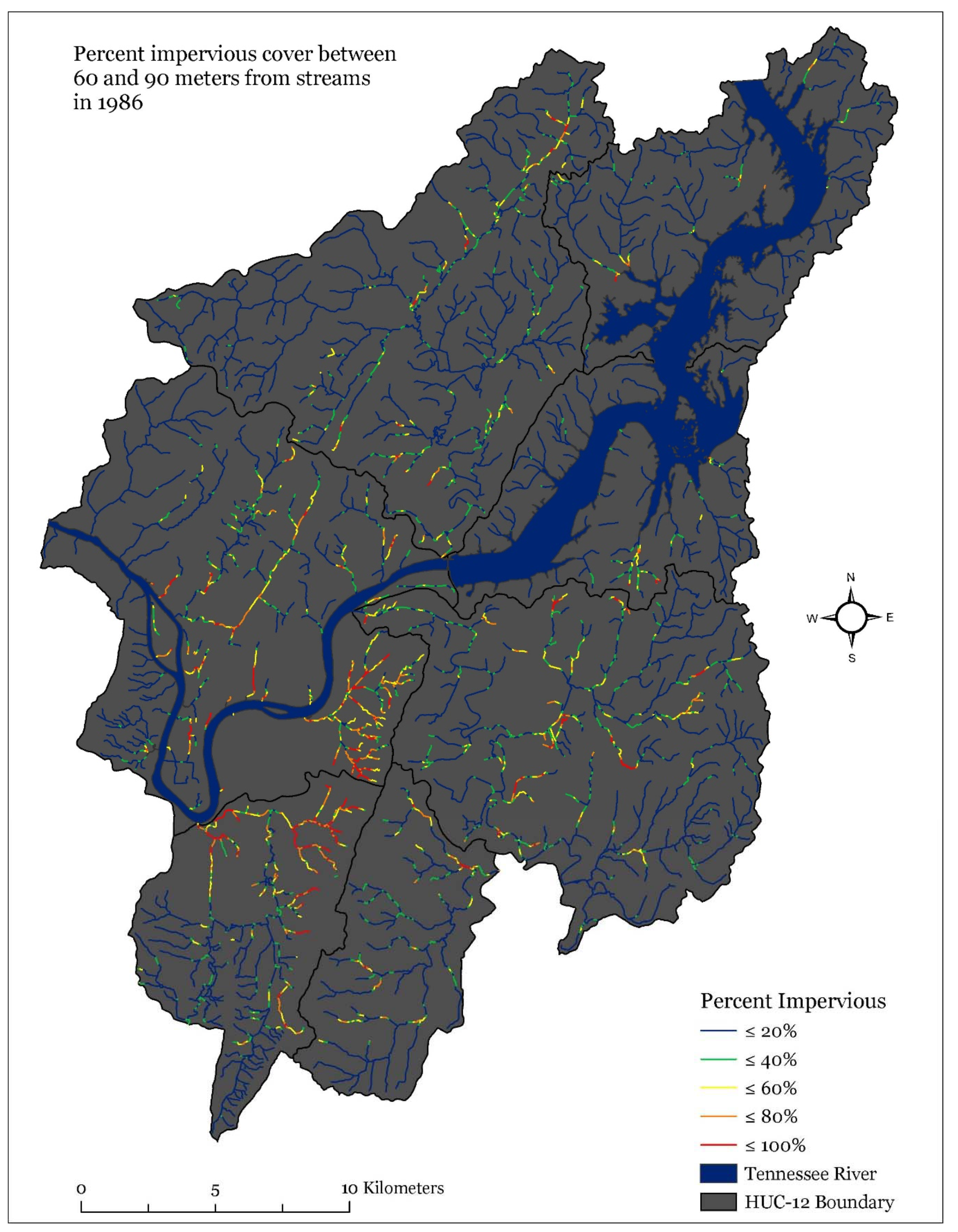
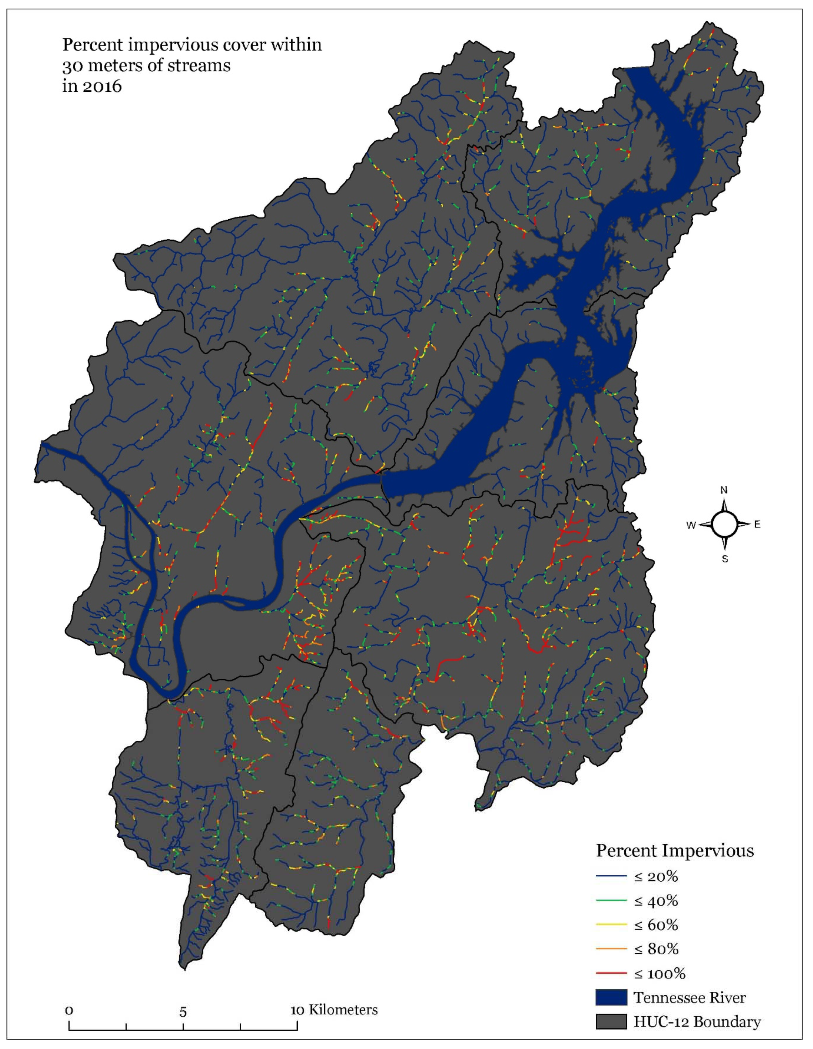
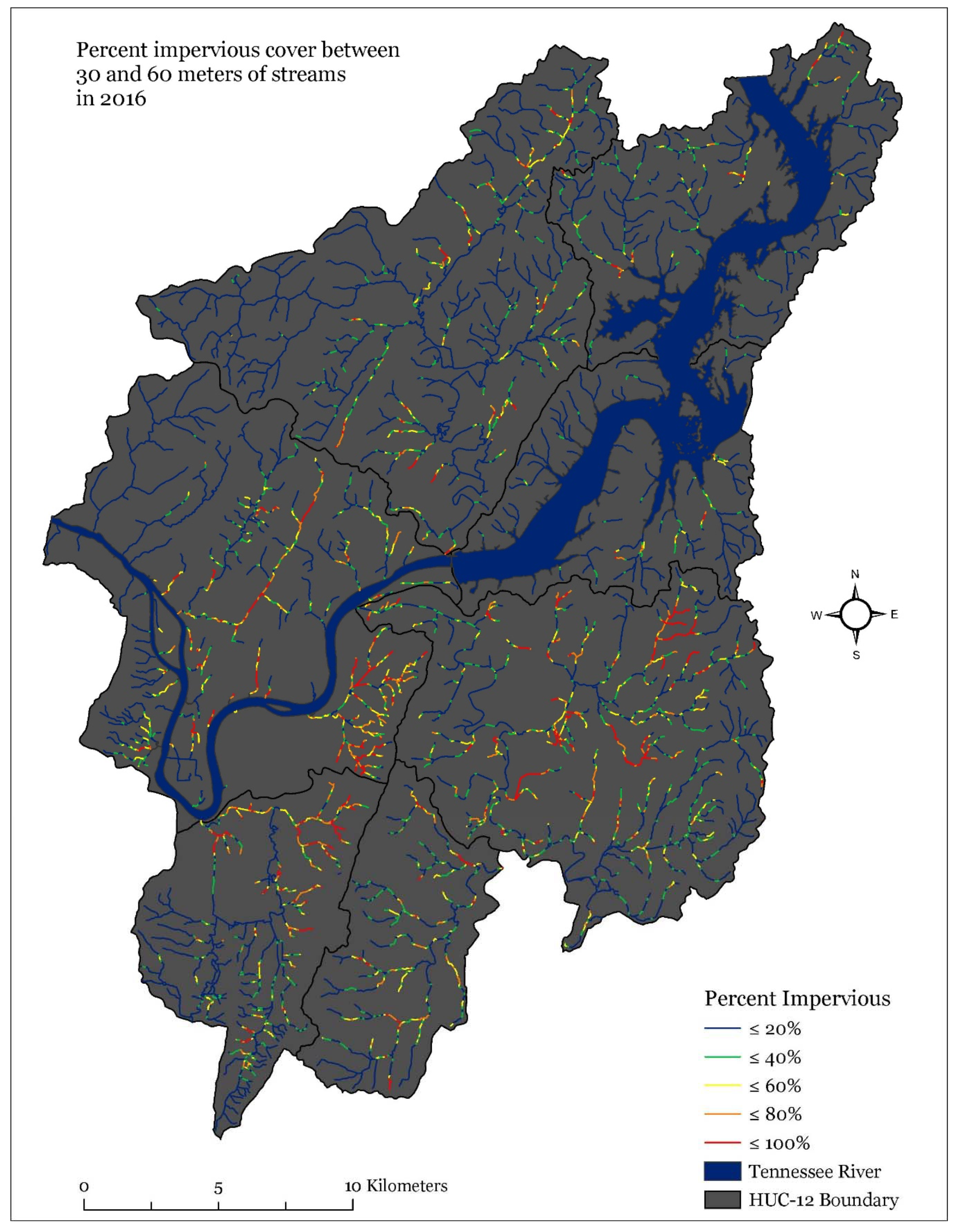
For the 1986 dataset, the first two 30 m riparian interval zones on average were 15.2% covered by IS with the third interval having an average of 15.5%. In the 2016 dataset, the average percent impervious cover for all the 30 m riparian zones had increased to 17.9%, 20.1%, and 21.6% respectively, with the amount of growth increasing for further riparian zones. Descriptive statistics for the riparian development analysis can be seen in

Table 8. Descriptive statistics for the percent imperviousness within the first three separate 30 m riparian zones for stream segments for 24 January 1986 and 26 November 2016.

Interval	Year	Mean	Standard Deviation	Quartile
				Min.	25%	50%	75%	Max.
0 m–30 m
	1986	15.2%	27.4%	0.0%	0.0%	0.0%	20.0%	100%
	2016	17.9%	29.8%	0.0%	0.0%	0.0%	25.0%	100%
30 m–60 m
	1986	15.2%	24.1%	0.0%	0.0%	0.0%	21.4%	100%
	2016	20.1%	27.7%	0.0%	0.0%	7.1%	33.3%	100%
60 m–90 m
	1986	15.5%	23.0%	0.0%	0.0%	5.2%	22.2%	100%
	2016	21.6%	27.0%	0.0%	0.0%	10.5%	35.7%	100%

. A visual description of the distributions of percent imperviousness for each zone in 1986 and 2016 can be seen below in Figure 20 with outliers being visualized as plus symbols above the top whisker. The distributions also show that the two further riparian zones show increases in the second and third quartiles compared to 1986. Maps showing the percent imperviousness for each riparian zone can be found in Appendix A (Figure A1, Figure A2, Figure A3, Figure A4, Figure A5 and Figure A6).

3.3.2. Stream Risk Assessment

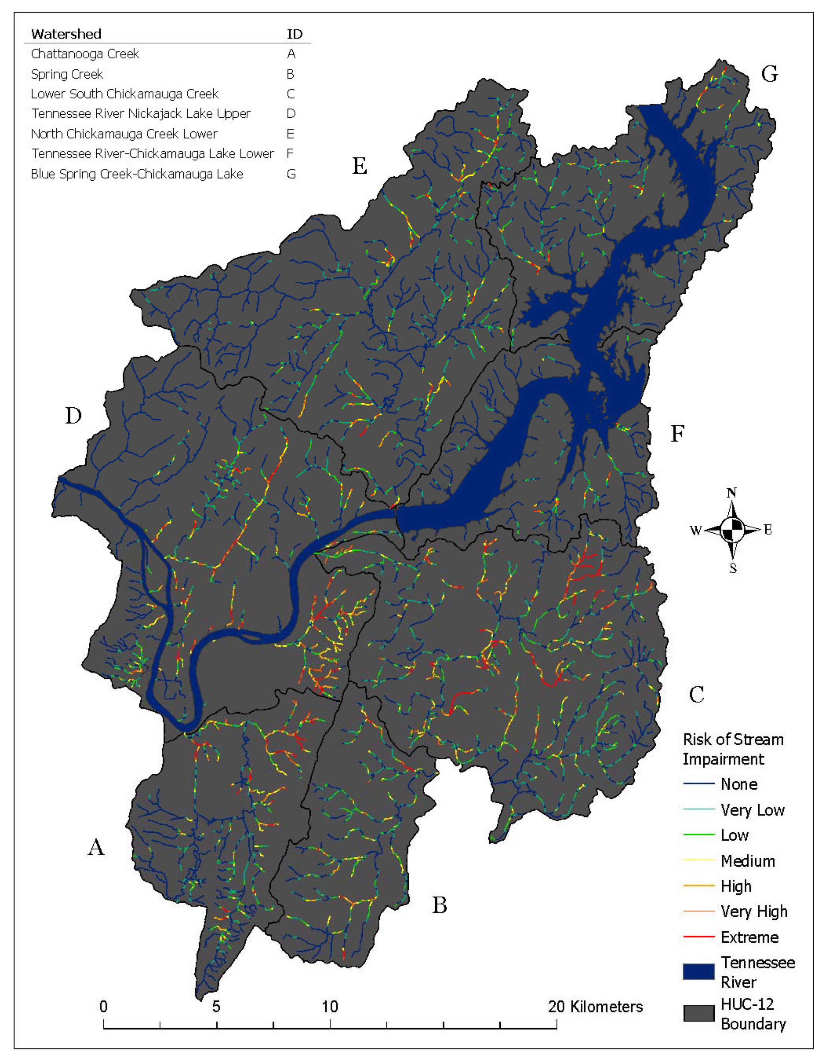
The range in values for the stream impairment risk model was 0 through 6, allowing for different levels of probable risk to be assigned.

Table 9. Model scores for potential stream risk assessments due to riparian imperviousness.

Risk of Impairment	Model Score
None	0 < 1
Very Low	≥1 < 2
Low	≥2 < 3
Medium	≥3 < 4
High	≥4 < 5
Very High	≥5 < 6
Extreme	6

shows the levels of risk related to the equivalent range in risk model values. The basis for these levels originated from the amount of development that must be present to achieve this score. For a stream segment to be assigned the lowest value (0.0) there must be 0% imperviousness in all three riparian zones while the maximum value (6.0) requires 100% imperviousness in all three riparian zones. Therefore, a score between 0 and 1 shows a stream segment with little to no risk of impairment related to IS development. A score between 5 and 6 shows areas that have significant impervious surfaces in their riparian zones, and thereby should have higher risk of impairment related to IS development. Figure 21 and Figure 22 show the possible risk of stream impairments due to IS development for 1986 and 2016, respectively.

The average score per stream segment was 0.92 and 1.06 for 1986 and 2016, respectively. Statistics describing the distribution of the model’s results are shown below in

Table 10. Statistics of potential risk assessment of stream segments due to riparian imperviousness.

			Quartile
Year	Mean	Standard Deviation	Min.	25%	50%	75%	Max.
1986	0.92	1.45	0	0	0.15	1.22	6
2016	1.06	1.47	0	0	0.33	1.57	6

. For both dates, 75% of the model scores were below 2, a classification of low risk of impairment.

Table 11. Stream impairment risk model score counts and approximate total stream lengths per score for each date. Counts represent the number of segments within that class.

Risk of Impairment	1986 (km)	2016 (km)	Change (km)
None	8155 (634)	7168 (550)	−987 (84)
Very Low	1883 (148)	2108 (169)	+225 (21)
Low	1012 (77)	1278 (100)	+266 (23)
Medium	737 (58)	812 (63)	+75 (5)
High	506 (36)	593 (45)	+87 (9)
Very High	374 (27)	505 (38)	+131 (11)
Extreme	243 (17)	446 (32)	+203 (15)

gives the quantity of segments with each level of risk, the total length of segments for each level of risk, and the change in quantities between 1986 and 2016. The distributions of risk scores for both dates can be visualized in boxplots shown in Figure 23.

4. Discussions

This study aimed to: (1) estimate and map the net impervious surface (IS) change in and around the City of Chattanooga, Tennessee, between 1986 and 2016 using satellite imagery from NASA’s Landsat satellite missions, (2) perform a quantitative analysis of the obtained IS changes in relation to local water resources, and (3) develop a risk assessment model to identify the potential areas of concern for surface water quality in the study site due to the proximity and quantity of IS growth. All three tasks were successfully completed in a reasonable sense. However, there were challenges associated with each task that should be taken into consideration to evaluate the outcome of this study. The important aspects of the obtained results for each task along with the limitations and challenges encountered are discussed in the following sections.

4.1. Impervious Surface (IS) Mapping

This study shows that there has been an overall increase in the net IS development between 1986 and 2016 within the study site. This amount of IS growth fits the substantial growth in population, housing units, and economic activity in the area, as other research has found that increases in population can be related to proportionally larger increases in IS [155,156]. The larger proportional increase in IS area could be viewed as the result of residential and commercial development driven by the population growth in the greater Chattanooga areas. The contribution of both population and economic growth to IS growth are considered for the EPA’s IS Growth Model [157]. The results are further supported by the EPA’s IS Growth Model since the three primary contributors to IS cover are buildings, roads, and parking lots, listed in order of contribution [157].

4.2. Impervious Surface (IS) Classification Accuracy

The results of the confusion matrix accuracy assessments show that the classification of impervious and non-impervious surfaces using the model developed in this study was reasonably successful. The model’s classification accuracy for pervious surfaces for both dates are much higher than impervious surfaces, which could result from the assignment of points using the random stratification method, which placed a much larger number of accuracy assessment points for assessing the pervious surfaces. The lower quantity of assessment points in impervious surfaces could, therefore, be more heavily affected by outlying classification errors. Differences in the User’s Accuracy and Producer’s Accuracy show the variation of different types of errors that the classification model experienced for each class. Having a higher Producer’s Accuracy shows that the model was more likely to have more false positives and less false negatives. On the other hand, a higher User’s Accuracy indicates the presence of the opposites [154]. In this study, for IS classification, both dates showed a higher Producer’s Accuracy. This result indicates that the model had a difficulty to differentiate between subject’s spectral responses effectively and consistently and, as a result, classified some non-urban areas as urban IS. The main source of confusion is believed to be derived from areas covered with open dry soils.

The zonal statistics accuracy assessments show that both dates had a similar performance in IS classification. This indicates the ability of the model to correctly classify moderately sized urban areas using both Landsat 5 TM and Landsat 8 OLI imagery.

4.3. Water Resource Proximity to Impervious Surfaces

The accuracy of the proximity of the impervious surface (IS) development to streams accuracy is dependent on the accuracy of the detected IS and the positional accuracy of the stream data, since the locations of the streams are assumed to be accurate due to the U.S. National Map accuracy standards met by the NHDplus dataset [68]. Errors from the IS detection portion of this study are believed to be the cause of the detected decrease in IS with 30 m of streams in the Chattanooga Creek and North Chickamauga Creek Lower watersheds and within 60 m of streams for the Chattanooga Creek watersheds. The results of the IS growth near streams also show that the growth is unequal across HUC-12 watersheds, thereby signifying that some may have increased impairment. This study shows that the Lower South Chickamauga watershed experienced the largest amount of urban growth between 1986 and 2016. This finding parallels with the finding that the Lower South Chickamauga watershed includes the largest amount of overall IS growth. Having the largest portion of IS development within the watershed and near the streams suggests that the Lower South Chickamauga watershed surface water quality could have the most noticeable and significant impairment relative to the other watersheds within the study site.

Differences in percent imperviousness between the three riparian zones show an average increase for all three zones with the increase being larger in the distant riparian zones. Shifting in the second and the third quartile percent imperviousness in the 2016 dataset compared to the 1986 dataset supported the conclusion that in 2016, stream riparian zones had experienced increases in IS development. The largest increases in the farthest zone suggests that the growth has begun to develop closer to streams. Increases in anthropogenic development and activity closer to streams increases the risk of potential impairment of stream surface water quality and riparian habitat [152]. Large portions of stream riparian zones are still present and not heavily disturbed within the study site. However, the findings of this research clearly shows the need for local policy action for riparian zone protection that could help mitigate the potential increase in stream impairment.

4.4. Impairment Risk Due to IS Development

The potential risk of stream impairment increased from 1986 to 2016. The increase in the total number of stream segments at risk being impaired suggested that stream surface water quality health in 2016 was at a higher risk than it was in 1986. Segments with extreme risk of impairment experienced the third largest increase between the two datasets. The increase in average risk can be attributed to the increase of risk for 7.64% of stream segments, where 987 stream segments have experienced increases in risk. This is coupled with the 27.75% of segments that have maintained risk of impairment since 1986. These findings show that there is a moderate proportion of streams within the study site that could have significant impairment due to long-term exposure or rapid introduction to urban development.

The risk model developed in this research showed that the locations of the potentially impaired stream segments due to impervious surface development are within the immediate riparian areas.

4.5. Limitations and Challenges

The accuracy assessment results for both datasets are at an acceptable level with regards to the effectiveness of the data and environmental conditions at the time of data acquisition. Moderate scale resolution sensors, such as the Landsat Thematic Mapper (TM) and Operational Land Imager (OLI), have been utilized for mapping impervious surfaces (IS), however, a consensus has been found that with data of this scale, it is not an effective ability to detect smaller areas of IS [158]. This study found that pixels determined as being IS are those where the majority to entirety of the land cover is impervious.

Environmental factors at the time of image acquisition are believed to have been an influence for both IS dataset generation. Water, shadow, and dry soil have been found to be difficult for many classification models due to the spectral confusion [159]. Shadows, which are present in both images, can be caused by the angle of the sun and/or sensor. The effect of shadowed areas was accounted for in the model and is not believed to have had any significant effect on the results of the study. For the 2016 image, a strong drought affected the study site and produced an increased amount of dry soils, river recession, and wildfires [160]. For the 1986 image, several clear-cut areas were seen in the study site exposing large areas of dry soil. The evaluation of the obtained IS data shows the presence of some dry and compacted soil, which were classified as IS. This probably stems from the conflicting spectral response of dry soil and IS (in some cases). However, it is believed that detection of dry soils as IS, in some cases, did not contribute to a major portion of detected areas [161,162].

The effects of noise and errors from the data, model, and environmental systems are also believed to have an influence on the results. The estimated area of IS for both dates is believed to be conservative, even with the detection of dry soil as it is inferred through the increase in housing units and population in the study site. There has been a net growth of suburban areas between 1986 and 2016, much of which is believed to have not been detected by this model based on visual inspection of the true color images. Suburban land cover can include IS such as roofs, drive-ways, and sidewalks. Although attempts were made to detect IS in suburban areas with the aid of true color images, it was not possible to accurately detect them due to sensor’s coarser spatial resolution and erroneous detection of dry soil.

5. Conclusions

This study successfully utilized remote sensing and GIS technologies to estimate and map historical and current impervious surfaces (IS) of the greater Chattanooga area to determine its net spatial growth across seven HUC-12 watersheds and their relationship to the streams. IS cover was used to represent areas of anthropogenic development, specifically urban and suburban areas. Utilizing the multispectral satellite imagery acquired by the USGS Landsat 5 and 8 programs, IS detection was conducted using the Normalized Difference Vegetation Index (NDVI) and density slicing technique. This study found that there had been a net increase in IS within the study site with significant growth occurring near many of the streams. The IS change estimation showed that the overall growth was not equally distributed. Most of the IS development occurred in the Lower South Chickamauga Creek watershed. It was found that dry soil from transitioning land cover or drought caused erroneous detection of IS in some cases. Areas of suburban development are not believed to be fully mapped due to the spectral dominance of the pervious surfaces such as tree cover.

The results of the stream - IS proximity analysis show that there is an overall increase in percent imperviousness surface growth in the first three 30 m stream riparian zones in the study site. The largest increase in percent imperviousness of stream riparian zone occurred between 60 m to 90 m from streams, indicating that urban growth is beginning to encroach on critical, immediate riparian zones. The model for potential risk of stream surface water quality impairment reflects that there is an increase in risk for some portions of the streams due to riparian IS development. The HUC-12 watersheds in the study site directly feed into the Tennessee River, thereby increasing the possible impact of the land use and cover change for areas downstream of the study site. This study also found that decreases in pervious surfaces in stream riparian zones signaled a decrease in buffer capacity for filtering impaired surface and ground water. IS development detected within the watersheds could be the sources of potential new or continued surface water quality degradation. Finally, this study can conclude that between 1986 and 2016, there was an increase of at least 45.12 km² of IS cover in the seven HUC-12 watersheds within the greater Chattanooga, Tennessee, area and 9.96 km² of this growth were within close proximity of the streams, which should cause concerns for the local stream and river surface water quality.

References

1. Chithra, S.; Nair, M.H.; Amarnath, A.; Anjana, N. Impacts of impervious surfaces on the environment. Int. J. Eng. Sci. Invent. 2015, 4, 2319–6726. [Google Scholar]
2. Barnes, K.B.; Morgan, J.; Roberge, M. Impervious surfaces and the quality of natural and built environments. In Department of Geography and Environmental Planning; Towson University: Baltimore, MD, USA, 2001. [Google Scholar]
3. United Nations Department of Economic and Social Affairs, P.D. World Urbanization Prospects: The 2014 Revision; ST/ESA/SER.A/366. 2015. Available online: https://www.un.org/en/development/desa/publications/2014-revision-world-urbanization-prospects.html (accessed on 28 February 2020).
4. Madlener, R.; Sunak, Y. Impacts of urbanization on urban structures and energy demand: What can we learn for urban energy planning and urbanization management? Sustain. Cities Soc. 2011, 1, 45–53. [Google Scholar] [CrossRef]
5. Li, B.Z.; Yao, R.M. Urbanization and its impact on building energy consumption and efficiency in China. Renew. Energy 2009, 34, 1994–1998. [Google Scholar] [CrossRef]
6. Li, K.; Lin, B.Q. Impacts of urbanization and industrialization on energy consumption/CO2 emissions: Does the level of development matter? Renew. Sustain. Energy Rev. 2015, 52, 1107–1122. [Google Scholar] [CrossRef]
7. Liddle, B. Impact of population, age structure, and urbanization on carbon emissions/energy consumption: Evidence from macro-level, cross-country analyses. Popul. Environ. 2014, 35, 286–304. [Google Scholar] [CrossRef] [Green Version]
8. Satterthwaite, D.; McGranahan, G.; Tacoli, C. Urbanization and its implications for food and farming. Philos. Trans. R. Soc. B Biol. Sci. 2010, 365, 2809–2820. [Google Scholar] [CrossRef] [PubMed]
9. Nizeyimana, E.L.; Petersen, G.W.; Imhoff, M.L.; Sinclair, H.R.; Waltman, S.W.; Reed-Margetan, D.S.; Levine, E.R.; Russo, J.M. Assessing the impact of land conversion to urban use on soils with different productivity levels in the USA. Soil Sci. Soc. Am. J. 2001, 65, 391–402. [Google Scholar] [CrossRef]
10. Szabo, S. Urbanization and food insecurity risks: Assessing the role of human development. Oxf. Dev. Stud. 2016, 44, 28–48. [Google Scholar] [CrossRef] [Green Version]
11. Huang, S.L.; Yeh, C.T.; Chang, L.F. The transition to an urbanizing world and the demand for natural resources. Curr. Opin. Environ. Sustain. 2010, 2, 136–143. [Google Scholar] [CrossRef]
12. Barlow, S.A.; Munn, I.A.; Cleaves, D.A.; Evans, D.L. The effect of urban sprawl on timber. J. For. 1998, 96, 10–14. [Google Scholar]
13. Munn, I.A.; Barlow, S.A.; Evans, D.L.; Cleaves, D. Urbanization's impact on timber harvesting in the south central United States. J. Environ. Manag. 2002, 64, 65–76. [Google Scholar] [CrossRef]
14. Nowak, D.J.; Walton, J.T. Projected urban growth (2000–2050) and its estimated impact on the US forest resource. J. For. 2005, 103, 383–389. [Google Scholar]
15. Putro, B.; Kjeldsen, T.R.; Hutchins, M.G.; Miller, J. An empirical investigation of climate and land-use effects on water quantity and quality in two urbanizing catchments in the southern United Kingdom. Sci. Total Environ. 2016, 548, 164–172. [Google Scholar] [CrossRef] [PubMed] [Green Version]
16. Zipper, S.C.; Soylu, M.E.; Kucharik, C.J.; Loheide, S.P. Quantifying indirect groundwater-mediated effects of urbanization on agroecosystem productivity using modflow-agroibis (MAGI), a complete critical zone model. Ecol. Model. 2017, 359, 201–219. [Google Scholar] [CrossRef]
17. Black, D.; Black, J. A review of the urban development and transport impacts on public health with particular reference to Australia: Trans-disciplinary research teams and some research gaps. Int. J. Environ. Res. Public Health 2009, 6, 1557–1596. [Google Scholar] [CrossRef] [PubMed] [Green Version]
18. Liu, Z.H.; Wang, Y.L.; Li, Z.G.; Peng, J. Impervious surface impact on water quality in the process of rapid urbanization in Shenzhen, China. Environ. Earth Sci. 2013, 68, 2365–2373. [Google Scholar] [CrossRef]
19. Xian, G.; Crane, M. Assessments of urban growth in the Tampa Bay watershed using remote sensing data. Remote Sens. Environ. 2005, 97, 203–215. [Google Scholar] [CrossRef]
20. Tu, J.; Xia, Z.G.; Clarke, K.C.; Frei, A. Impact of urban sprawl on water quality in eastern Massachusetts, USA. Environ. Manag. 2007, 40, 183–200. [Google Scholar] [CrossRef]
21. Arnold, C.L., Jr.; Gibbons, C.J. Impervious surface coverage: The emergence of a key environmental indicator. J. Am. Plan. Assoc. 1996, 62, 243–258. [Google Scholar] [CrossRef]
22. Du, N.; Ottens, H.; Sliuzas, R. Spatial impact of urban expansion on surface water bodies—A case study of Wuhan, China. Landsc. Urban Plan. 2010, 94, 175–185. [Google Scholar] [CrossRef]
23. Todd, D.A.; Bedient, P.B.; Haasbeek, J.F.; Noell, J. Impact of land-use and NPS loads on lake quality. J. Environ. Eng. ASCE 1989, 115, 633–649. [Google Scholar] [CrossRef]
24. Carle, M.V.; Halpin, P.N.; Stow, C.A. Patterns of watershed urbanization and impacts on water quality. J. Am. Water Resour. Assoc. 2005, 41, 693–708. [Google Scholar] [CrossRef]
25. Price, K.; Leigh, D.S. Comparative water quality of lightly-and moderately-impacted streams in the southern Blue Ridge Mountains, USA. Environ. Monit. Assess. 2006, 120, 269–300. [Google Scholar] [CrossRef] [PubMed]
26. Brett, M.T.; Arhonditsis, G.B.; Mueller, S.E.; Hartley, D.M.; Frodge, J.D.; Funke, D.E. Non-point-source impacts on stream nutrient concentrations along a forest to urban gradient. Environ. Manag. 2005, 35, 330–342. [Google Scholar] [CrossRef]
27. Teixeira, L.C.; de Paiva, J.B.D.; Pereira, J.E.D.; Lisboa, R.D. Relationship between turbidity and suspended sediment concentration from a small hydrographic basin in Santa Maria (Rio Grande do Sul, Brazil). Int. J. River Basin Manag. 2016, 14, 393–399. [Google Scholar] [CrossRef]
28. Tu, J. Spatially varying relationships between land use and water quality across an urbanization gradient explored by geographically weighted regression. Appl. Geogr. 2011, 31, 376–392. [Google Scholar] [CrossRef]
29. Tong, S.T.Y.; Chen, W.L. Modeling the relationship between land use and surface water quality. J. Environ. Manag. 2002, 66, 377–393. [Google Scholar] [CrossRef]
30. Tu, J. Spatial variations in the relationships between land use and water quality across an urbanization gradient in the watersheds of Northern Georgia, USA. Environ. Manag. 2013, 51, 1–17. [Google Scholar] [CrossRef]
31. May, C.W.; Horner, R.R.; Karr, J.R.; Mar, B.W.; Welch, E.B. Effects of urbanization on small streams in the Puget sound ecoregion. Watershed Prot. Tech. 1999, 2, 79. [Google Scholar]
32. Yang, L.; Ma, K.M.; Gua, Q.H.; Bai, X. Evaluating long-term hydrological impacts of regional urbanization in Hanyang, China, using a GIS model and remote sensing. Int. J. Sustain. Dev. World Ecol. 2008, 15, 350–356. [Google Scholar] [CrossRef]
33. Williams, M.; Hopkinson, C.; Rastetter, E.; Vallino, J.; Claessens, L. Relationships of land use and stream solute concentrations in the Ipswich River basin, northeastern Massachusetts. Water Air Soil Pollut. 2005, 161, 55–74. [Google Scholar] [CrossRef]
34. Horner, R.R.; Booth, D.B.; Azous, A.; May, C.W. Watershed determinants of ecosystem functioning. In Proceedings of the Effects of Watershed Development and Management on Aquatic Ecosystems, New York, NY, USA, 4–9 August 1996; pp. 251–274. [Google Scholar]
35. Long, J.; Schorr, M.S. Effects of watershed urban land use on environmental conditions and fish assemblages in Chattanooga area streams (Tennessee-Georgia). J. Freshw. Ecol. 2005, 20, 527–537. [Google Scholar] [CrossRef]
36. Nagy, R.C.; Lockaby, B.G.; Kalin, L.; Anderson, C. Effects of urbanization on stream hydrology and water quality: The Florida Gulf Coast. Hydrol. Process. 2012, 26, 2019–2030. [Google Scholar] [CrossRef]
37. Poole, G.C.; Berman, C.H. An ecological perspective on in-stream temperature: Natural heat dynamics and mechanisms of human-caused thermal degradation. Environ. Manag. 2001, 27, 787–802. [Google Scholar] [CrossRef] [PubMed]
38. Wang, J.; Da, L.; Song, K.; Li, B.-L. Temporal variations of surface water quality in urban, suburban and rural areas during rapid urbanization in Shanghai, China. Environ. Pollut. 2008, 152, 387–393. [Google Scholar] [CrossRef] [PubMed]
39. Conway, T.M. Impervious surface as an indicator of pH and specific conductance in the urbanizing coastal zone of New Jersey, USA. J. Environ. Manag. 2007, 85, 308–316. [Google Scholar] [CrossRef] [PubMed]
40. Martins, R.T.; Couceiro, S.R.M.; Melo, A.S.; Moreira, M.P.; Hamada, N. Effects of urbanization on stream benthic invertebrate communities in central Amazon. Ecol. Ind. 2017, 73, 480–491. [Google Scholar] [CrossRef]
41. Mancini, L.; Formichetti, P.; D’Angelo, A.M.; Pierdominici, E.; Sorace, A.; Bottoni, P.; Iaconelli, M.; Ferrari, C.; Tancioni, L.; Rossi, N.; et al. Freshwater quality in urban areas: A case study from Rome, Italy. Microchem. J. 2005, 79, 177–183. [Google Scholar] [CrossRef]
42. Sonneman, J.A.; Walsh, C.J.; Breen, P.F.; Sharpe, A.K. Effects of urbanization on streams of the Melbourne region, Victoria, Australia. II. Benthic diatom communities. Freshw. Biol. 2001, 46, 553–565. [Google Scholar] [CrossRef]
43. Almeida, C.A.; Quintar, S.; Gonzalez, P.; Mallea, M.A. Influence of urbanization and tourist activities on the water quality of the Potrero de los Funes River (San Luis Argentina). Environ. Monit. Assess. 2007, 133, 459–465. [Google Scholar] [CrossRef]
44. Desai, A.M.; Rifai, H.S. Variability of Escherichia coli Concentrations in an Urban Watershed in Texas. J. Environ. Eng. ASCE 2010, 136, 1347–1359. [Google Scholar] [CrossRef]
45. Chessman, B.; Growns, I.; Currey, J.; Plunkett-Cole, N. Predicting diatom communities at the genus level for the rapid biological assessment of rivers. Freshw. Biol. 1999, 41, 317–331. [Google Scholar] [CrossRef]
46. Hatt, B.E.; Fletcher, T.D.; Walsh, C.J.; Taylor, S.L. The influence of urban density and drainage infrastructure on the concentrations and loads of pollutants in small streams. Environ. Manag. 2004, 34, 112–124. [Google Scholar] [CrossRef] [PubMed]
47. Walsh, C.J.; Roy, A.H.; Feminella, J.W.; Cottingham, P.D.; Groffman, P.M.; Morgan, R.P. The urban stream syndrome: Current knowledge and the search for a cure. J. N. Am. Benthol. Soc. 2005, 24, 706–723. [Google Scholar] [CrossRef]
48. Homer, C.; Dewitz, J.; Fry, J.; Coan, M.; Hossain, N.; Larson, C.; Herold, N.; McKerrow, A.; VanDriel, J.N.; Wickham, J. Completion of the 2001 National Land Cover Database for the conterminous United States. Photogramm. Eng. Remote Sens. 2007, 73, 337–341. [Google Scholar]
49. Fry, J.; Xian, G.Z.; Jin, S.; Dewitz, J.; Homer, C.G.; Yang, L.; Barnes, C.A.; Herold, N.D.; Wickham, J.D. Completion of the 2006 national land cover database for the conterminous United States. Photogramm. Eng. Remote Sens. 2011, 77, 858–864. [Google Scholar]
50. Homer, C.; Dewitz, J.; Yang, L.M.; Jin, S.; Danielson, P.; Xian, G.; Coulston, J.; Herold, N.; Wickham, J.; Megown, K. Completion of the 2011 national land cover database for the conterminous united states—representing a decade of land cover change information. Photogramm. Eng. Remote Sens. 2015, 81, 345–354. [Google Scholar] [CrossRef]
51. Chen, Y.J.; Yu, S.X. Assessment of urban growth in Guangzhou using multi-temporal, multi-sensor Landsat data to quantify and map impervious surfaces. Int. J. Remote Sens. 2016, 37, 5936–5952. [Google Scholar] [CrossRef]
52. Shahtahmassebi, A.R.; Song, J.; Zheng, Q.; Blackburn, G.A.; Wang, K.; Huang, L.Y.; Pan, Y.; Moore, N.; Shahtahmassebi, G.; Haghighi, R.S.; et al. Remote sensing of impervious surface growth: A framework for quantifying urban expansion and re-densification mechanisms. Int. J. Appl. Earth Obs. Geoinf. 2016, 46, 94–112. [Google Scholar] [CrossRef] [Green Version]
53. Yang, L.M.; Xian, G.; Klaver, J.M.; Deal, B. Urban land-cover change detection through sub-pixel imperviousness mapping using remotely sensed data. Photogramm. Eng. Remote Sens. 2003, 69, 1003–1010. [Google Scholar] [CrossRef]
54. Jat, M.K.; Garg, P.K.; Khare, D. Monitoring and modelling of urban sprawl using remote sensing and GIS techniques. Int. J. Appl. Earth Obs. Geoinf. 2008, 10, 26–43. [Google Scholar] [CrossRef]
55. Chen, X.L.; Zhao, H.M.; Li, P.X.; Yin, Z.Y. Remote sensing image-based analysis of the relationship between urban heat island and land use/cover changes. Remote Sens. Environ. 2006, 104, 133–146. [Google Scholar] [CrossRef]
56. Seto, K.C.; Woodcock, C.E.; Song, C.; Huang, X.; Lu, J.; Kaufmann, R.K. Monitoring land-use change in the Pearl River Delta using Landsat TM. Int. J. Remote Sens. 2002, 23, 1985–2004. [Google Scholar] [CrossRef]
57. Weng, Q.H. Land use change analysis in the Zhujiang Delta of China using satellite remote sensing, GIS and stochastic modelling. J. Environ. Manag. 2002, 64, 273–284. [Google Scholar] [CrossRef] [PubMed] [Green Version]
58. Weng, Q. A remote sensing-GIS evaluation of urban expansion and its impact on surface temperature in the Zhujiang Delta, China. Int. J. Remote Sens. 2001, 22, 1999–2014. [Google Scholar] [CrossRef]
59. Wilson, E.H.; Hurd, J.D.; Civco, D.L.; Prisloe, M.P.; Arnold, C. Development of a geospatial model to quantify, describe and map urban growth. Remote Sens. Environ. 2003, 86, 275–285. [Google Scholar] [CrossRef]
60. Zha, Y.; Gao, J.; Ni, S. Use of normalized difference built-up index in automatically mapping urban areas from TM imagery. Int. J. Remote Sens. 2003, 24, 583–594. [Google Scholar] [CrossRef]
61. Xu, H. A new index for delineating built-up land features in satellite imagery. Int. J. Remote Sens. 2008, 29, 4269–4276. [Google Scholar] [CrossRef]
62. Yang, X.J.; Liu, Z. Using satellite imagery and GIS for land-use and land-cover change mapping in an estuarine watershed. Int. J. Remote Sens. 2005, 26, 5275–5296. [Google Scholar] [CrossRef]
63. Kauth, R.J.; Thomas, G. The Tasseled Cap—A graphic description of the spectral-temporal development of agricultural crops as seen by Landsat. In Proceedings of the LARS Symposia, West Lafayette, IN, USA, 29 June–1 July 1976; p. 159. [Google Scholar]
64. Rouse, J.W., Jr.; Haas, R.; Schell, J.; Deering, D. Monitoring vegetation systems in the Great Plains with ERTS. NASA Spec. Publ. 1974, 351, 309. [Google Scholar]
65. Hu, Z.Y. Using NDVI differencing and temporal logic to enhance ISODATA classification in urban environments. Gisci. Remote Sens. 2007, 44, 48–67. [Google Scholar] [CrossRef]
66. Osgouei, P.E.; Kaya, S. Analysis of land cover/use changes using Landsat 5 TM data and indices. Environ. Monit. Assess. 2017, 189, 136. [Google Scholar] [CrossRef] [PubMed]
67. Amirsalari, F.; Li, J.; Guan, X.; Booty, W.G. Investigation of correlation between remotely sensed impervious surfaces and chloride concentrations. Int. J. Remote Sens. 2013, 34, 1507–1525. [Google Scholar] [CrossRef] [Green Version]
68. Li, W.F.; Ouyang, Z.Y.; Zhou, W.Q.; Chen, Q.W. Effects of spatial resolution of remotely sensed data on estimating urban impervious surfaces. J. Environ. Sci. 2011, 23, 1375–1383. [Google Scholar] [CrossRef]
69. Turgeon, P.; Michel, P.; Levallois, P.; Ravel, A.; Archambault, M.; Lavigne, M.P.; Kotchi, S.O.; Brazeau, S. Assessing and monitoring agroenvironmental determinants of recreational freshwater quality using remote sensing. Water Sci. Technol. 2013, 67, 1503–1511. [Google Scholar] [CrossRef]
70. Hansen, B.; Reich, P.; Lake, P.S.; Cavagnaro, T. Minimum Width Requirements for Riparian Zones to Protect Flowing Waters and to Conserve Biodiversity: A Review and Recommendations; Monash University: Melbourne, Australia, 2010. [Google Scholar]
71. Smart, R.; Soulsby, C.; Cresser, M.; Wade, A.; Townend, J.; Billett, M.; Langan, S. Riparian zone influence on stream water chemistry at different spatial scales: A GIS-based modelling approach, an example for the Dee, NE Scotland. Sci. Total Environ. 2001, 280, 173–193. [Google Scholar] [CrossRef]
72. Peterjohn, W.T.; Correll, D.L. Nutrient dynamics in an agricultural watershed: Observations on the role of a riparian forest. Ecology 1984, 65, 1466–1475. [Google Scholar] [CrossRef]
73. Davies, P.; Nelson, M. Relationships between riparian buffer widths and the effects of logging on stream habitat, invertebrate community composition and fish abundance. Mar. Freshw. Res. 1994, 45, 1289–1305. [Google Scholar] [CrossRef]
74. Lowrance, R.; Altier, L.S.; Newbold, J.D.; Schnabel, R.R.; Groffman, P.M.; Denver, J.M.; Correll, D.L.; Gilliam, J.W.; Robinson, J.L.; Brinsfield, R.B.; et al. Water quality functions of Riparian forest buffers in Chesapeake Bay watershed. Environ. Manag. 1997, 21, 687–712. [Google Scholar] [CrossRef]
75. Schultz, R.C.; Isenhart, T.M.; Simpkins, W.W.; Colletti, J.P. Riparian forest buffers in agroecosystems—lessons learned from the Bear Creek Watershed, central Iowa, USA. Agrofor. Syst. 2004, 61, 35–50. [Google Scholar] [CrossRef]
76. Apan, A.A.; Raine, S.R.; Paterson, M.S. Mapping and analysis of changes in the riparian landscape structure of the Lockyer Valley catchment, Queensland, Australia. Landsc. Urban Plan. 2002, 59, 43–57. [Google Scholar] [CrossRef] [Green Version]
77. Mayer, P.M.; Reynolds, S.; Tim, C.; Mccutchen, M. Riparian Buffer Width, Vegetative Cover, and Nitrogen Removal Effectiveness: A Review of Current Science and Regulations; U.S. Environmental Protection Agency: Washington, DC, USA, 2005.
78. Goetz, S.J.; Wright, R.K.; Smith, A.J.; Zinecker, E.; Schaub, E. IKONOS imagery for resource management: Tree cover, impervious surfaces, and riparian buffer analyses in the mid-Atlantic region. Remote Sens. Environ. 2003, 88, 195–208. [Google Scholar] [CrossRef]
79. Tran, C.P.; Bode, R.W.; Smith, A.J.; Kleppel, G.S. Land-use proximity as a basis for assessing stream water quality in New York State (USA). Ecol. Ind. 2010, 10, 727–733. [Google Scholar] [CrossRef]
80. Paul, M.J.; Meyer, J.L. Streams in the urban landscape. Ann. Rev. Ecol. Syst. 2001, 32, 333–365. [Google Scholar] [CrossRef]
81. Osborne, L.L. Empirical relationship between land use/cover and stream water quality in an agricultural watershed. J. Environ. Manag. 1988, 26, 9–27. [Google Scholar]
82. Johnson, L.; Richards, C.; Host, G.; Arthur, J. Landscape influences on water chemistry in midwestern stream ecosystems. Freshw. Biol. 1997, 37, 193–208. [Google Scholar] [CrossRef]
83. Dodds, W.K.; Oakes, R.M. Headwater influences on downstream water quality. Environ. Manag. 2008, 41, 367–377. [Google Scholar] [CrossRef] [PubMed] [Green Version]
84. Schueler, T.R.; Fraley-McNeal, L.; Cappiella, K. Is impervious cover still important? Review of recent research. J. Hydrol. Eng. 2009, 14, 309–315. [Google Scholar]
85. Willis, K.S. Remote sensing change detection for ecological monitoring in United States protected areas. Biol. Conserv. 2015, 182, 233–242. [Google Scholar] [CrossRef]
86. Lu, D.; Mausel, P.; Brondizio, E.; Moran, E. Change detection techniques. Int. J. Remote Sens. 2004, 25, 2365–2407. [Google Scholar] [CrossRef]
87. Joshi, N.; Baumann, M.; Ehammer, A.; Fensholt, R.; Grogan, K.; Hostert, P.; Jepsen, M.R.; Kuemmerle, T.; Meyfroidt, P.; Mitchard, E.T.A.; et al. A Review of the application of optical and radar remote sensing data fusion to land use mapping and monitoring. Remote Sens. 2016, 8, 70. [Google Scholar] [CrossRef] [Green Version]
88. Hurtt, G.C.; Rosentrater, L.; Frolking, S.; Moore, B. Linking remote-sensing estimates of land cover and census statistics on land use to produce maps of land use of the conterminous United States. Glob. Biogeochem. Cycles 2001, 15, 673–685. [Google Scholar] [CrossRef]
89. Williams, D.L.; Goward, S.; Arvidson, T. Landsat: Yesterday, today, and tomorrow. Photogramm. Eng. Remote Sens. 2006, 72, 1171–1178. [Google Scholar] [CrossRef]
90. MacLachlan, A.; Biggs, E.; Roberts, G.; Boruff, B. Urban growth dynamics in perth, western Australia: Using applied remote sensing for sustainable future planning. Land 2017, 6, 9. [Google Scholar] [CrossRef] [Green Version]
91. Megahed, Y.; Cabral, P.; Silva, J.; Caetano, M. Land cover mapping analysis and urban growth modelling using remote sensing techniques in Greater Cairo Region-Egypt. ISPRS Int. J. Geo Inf. 2015, 4, 1750–1769. [Google Scholar] [CrossRef] [Green Version]
92. Chen, S.P.; Zeng, S.; Xie, C.G. Remote sensing and GIS for urban growth analysis in China. Photogramm. Eng. Remote Sens. 2000, 66, 593–598. [Google Scholar]
93. Ban, Y.F.; Yousif, O.A. Multitemporal Spaceborne SAR Data for Urban Change Detection in China. IEEE J. Sel. Top. Appl. Earth Obs. Remote Sens. 2012, 5, 1087–1094. [Google Scholar] [CrossRef]
94. Perissin, D.; Wang, T. Time-series INSAR applications over urban areas in China. IEEE J. Sel. Top. Appl. Earth Obs. Remote Sens. 2011, 4, 92–100. [Google Scholar] [CrossRef]
95. Han, R.M.; Liu, P.; Wang, H.; Yang, L.K.; Zhang, H.W.; Ma, C. An improved urban mapping strategy based on collaborative processing of optical and SAR remotely sensed data. Math. Probl. Eng. 2017. [Google Scholar] [CrossRef] [Green Version]
96. Corbane, C.; Faure, J.F.; Baghdadi, N.; Villeneuve, N.; Petit, M. Rapid urban mapping using SAR/optical imagery synergy. Sensors 2008, 8, 7125–7143. [Google Scholar] [CrossRef]
97. Zhang, X.P.; Pan, D.L.; Chen, J.Y.; Zhan, Y.Z.; Mao, Z.H. Using long time series of Landsat data to monitor impervious surface dynamics: A case study in the Zhoushan islands. J. Appl. Remote Sens. 2013, 7. [Google Scholar] [CrossRef] [Green Version]
98. Lu, D.S.; Moran, E.; Hetrick, S. Detection of impervious surface change with multitemporal Landsat images in an urban-rural frontier. ISPRS J. Photogramm. Remote Sens. 2011, 66, 298–306. [Google Scholar] [CrossRef] [PubMed] [Green Version]
99. Zhang, L.; Weng, Q.H. Annual dynamics of impervious surface in the Pearl River Delta, China, from 1988 to 2013, using time series Landsat imagery. ISPRS J. Photogramm. Remote Sens. 2016, 113, 86–96. [Google Scholar] [CrossRef]
100. Xian, G.; Crane, M.; McMahon, C. Quantifying multi-temporal urban development characteristics in Las Vegas from Landsat and ASTER data. Photogramm. Eng. Remote Sens. 2008, 74, 473–481. [Google Scholar] [CrossRef]
101. Wu, C.S.; Yuan, F. Seasonal sensitivity analysis of impervious surface estimation with satellite imagery. Photogramm. Eng. Remote Sens. 2007, 73, 1393–1401. [Google Scholar] [CrossRef] [Green Version]
102. Lu, D.S.; Weng, Q.H. Spectral mixture analysis of the urban landscape in Indianapolis with Landsat ETM plus imagery. Photogramm. Eng. Remote Sens. 2004, 70, 1053–1062. [Google Scholar] [CrossRef]
103. Weng, Q.H.; Hu, X.F. Medium spatial resolution satellite imagery for estimating and mapping urban impervious surfaces using LSMA and ANN. IEEE Trans. Geosci. Remote Sens. 2008, 46, 2397–2406. [Google Scholar] [CrossRef]
104. Weng, Q.H.; Hu, X.F.; Liu, H. Estimating impervious surfaces using linear spectral mixture analysis with multitemporal ASTER images. Int. J. Remote Sens. 2009, 30, 4807–4830. [Google Scholar] [CrossRef]
105. Rashed, T.; Weeks, J.R.; Roberts, D.; Rogan, J.; Powell, R. Measuring the physical composition of urban morphology using multiple endmember spectral mixture models. Photogramm. Eng. Remote Sens. 2003, 69, 1011–1020. [Google Scholar] [CrossRef] [Green Version]
106. Rodriguez-Galiano, V.F.; Ghimire, B.; Rogan, J.; Chica-Olmo, M.; Rigol-Sanchez, J.P. An assessment of the effectiveness of a random forest classifier for land-cover classification. ISPRS J. Photogramm. Remote Sens. 2012, 67, 93–104. [Google Scholar] [CrossRef]
107. Chen, Y.S.; Lin, Z.H.; Zhao, X.; Wang, G.; Gu, Y.F. Deep learning-based classification of hyperspectral data. IEEE J. Sel. Top. Appl. Earth Obs. Remote Sens. 2014, 7, 2094–2107. [Google Scholar] [CrossRef]
108. Schneider, A. Monitoring land cover change in urban and pen-urban areas using dense time stacks of Landsat satellite data and a data mining approach. Remote Sens. Environ. 2012, 124, 689–704. [Google Scholar] [CrossRef]
109. Im, J.; Jensen, J.R.; Tullis, J.A. Object-based change detection using correlation image analysis and image segmentation. Int. J. Remote Sens. 2008, 29, 399–423. [Google Scholar] [CrossRef]
110. Zhu, X.X.; Tuia, D.; Mou, L.; Xia, G.-S.; Zhang, L.; Xu, F.; Fraundorfer, F. Deep learning in remote sensing: A review. arXiv 2017, arXiv:1710.03959. [Google Scholar]
111. Kucsicsa, G.; Grigorescu, I. Urban growth in the Bucharest metropolitan area: Spatial and temporal assessment using logistic regression. J. Urban Plan. Dev. 2018, 144, 05017013. [Google Scholar] [CrossRef]
112. Zhang, L.; Wei, Y.H.D.; Meng, R. Spatiotemporal dynamics and spatial determinants of urban growth in Suzhou, China. Sustainability 2017, 9, 393. [Google Scholar] [CrossRef] [Green Version]
113. Roy, A.H.; Rosemond, A.D.; Paul, M.J.; Leigh, D.S.; Wallace, J.B. Stream macroinvertebrate response to catchment urbanization (Georgia, USA). Freshw. Biol. 2003, 48, 329–346. [Google Scholar] [CrossRef]
114. Arsanjani, J.J.; Helbich, M.; Kainz, W.; Boloorani, A.D. Integration of logistic regression, Markov chain and cellular automata models to simulate urban expansion. Int. J. Appl. Earth Obs. Geoinf. 2013, 21, 265–275. [Google Scholar] [CrossRef]
115. Luo, J.; Yu, D.; Xin, M. Modeling urban growth using GIS and remote sensing. Gisci. Remote Sens. 2008, 45, 426–442. [Google Scholar] [CrossRef]
116. Lary, D.J.; Alavi, A.H.; Gandomi, A.H.; Walker, A.L. Machine learning in geosciences and remote sensing. Geosci. Front. 2016, 7, 3–10. [Google Scholar] [CrossRef] [Green Version]
117. VanderPlas, J. Python Data Science Handbook: Essential Tools for Working with Data; O’Reilly Media, Inc.: Sevastopol, CA, USA, 2016. [Google Scholar]
118. Cracknell, M.J.; Reading, A.M. Geological mapping using remote sensing data: A comparison of five machine learning algorithms, their response to variations in the spatial distribution of training data and the use of explicit spatial information. Comput. Geosci. 2014, 63, 22–33. [Google Scholar] [CrossRef] [Green Version]
119. Hassan, M.M.; Southworth, J. Analyzing land cover change and urban growth trajectories of the mega-urban region of Dhaka using remotely sensed data and an ensemble classifier. Sustainability 2018, 10, 10. [Google Scholar] [CrossRef] [Green Version]
120. Goldblatt, R.; You, W.; Hanson, G.; Khandelwal, A.K. Detecting the boundaries of urban areas in India: A dataset for pixel-based image classification in google earth engine. Remote Sens. 2016, 8, 34. [Google Scholar] [CrossRef] [Green Version]
121. Sohn, P. Creek Pollution Stirs New Debate; The Times Free Press: Chattanooga, TN, USA, 2010. [Google Scholar]
122. Schorr, M.; Crews, E.; Freeman, P.; Long, J.; Johnson, P.; Fritz, D. Assessment of Water Quality and Aquatic Macrofauna in Chattanooga Area Streams, Contract No. R04101154-64. Final Report; City of Chattanooga, Department of Public Works, Stormwater Management Section: Chattanooga, TN, USA, 2001. [Google Scholar]
123. Flessner, D. Tourism Pumped $1 Billion into Chattanooga Economy in 2015; The Times Free Press: Chattanooga, TN, USA, 2016. [Google Scholar]
124. Flessner, D. Hamilton County Is Growing 25 Percent Faster than Tennessee as a Whole; The Times Free Press: Chattanooga, TN, USA, 2017. [Google Scholar]
125. Flessner, D. Chattanooga among Top 25 Cities for Job Growth This Year; The Times Free Press: Chattanooga, TN, USA, 2017. [Google Scholar]
126. Marinova, P. One of America’s Most Startup-Friendly Cities Is in Tennessee; Fortune: New York, NY, USA, 2017. [Google Scholar]
127. Tennessee Office of the Governor. Haslam Appoints Steering Committee to Develop Statewide Plan for Future Water Availability. Available online: https://www.tn.gov/governor/news/2018/1/18/haslam-appoints-steering-committee-to-develop-statewide-plan-for-future-water-availability.html (accessed on 2 September 2018).
128. Boyd Center for Business and Economic Research. Annual Tennessee MSA Population Projection Totals: 2016–2070. University of Tennessee, K., Ed. 2017. Available online: https://tnsdc.utk.edu/estimates-and-projections/boyd-center-population-projections/ (accessed on 28 February 2020).
129. Pare, M. Chattanooga to Gain from More Auto Production in Region, Experts Say; The Times Free Press: Chattanooga, TN, USA, 2018. [Google Scholar]
130. McClane, J. More Growth is Headed Chattanooga’s Way, But Some Residents Have Concerns; The Times Free Press: Chattanooga, TN, USA, 2018. [Google Scholar]
131. Cofer, B. Gross to Green: City Makes Strides to Becoming Sustainable; The Times Free Press: Chattanooga, TN, USA, 2011. [Google Scholar]
132. Sohn, P. Chattanooga Creek Still Threatened; The Times Free Press: Chattanooga, TN, USA, 2010. [Google Scholar]
133. U.S. Census Bureau. 2010 Census Gazetteer Files. 2012. Available online: https://www2.census.gov/geo/docs/maps-data/data/gazetteer/counties_list_47.txt (accessed on 28 February 2020).
134. Griffith, G.E.; Omernik, J.M.; Azevedo, S.H. Ecoregions of Tennessee; EPA/600/R-97/022; U.S. Environmental Protection Agency, National Health and Environmental Effects Research Laboratory: Corvallis, OR, USA, 2002; 51p. Available online: https://store.usgs.gov/assets/MOD/StoreFiles/Ecoregion/21632_tn_front.pdf (accessed on 28 February 2020).
135. Swingle, G.D. An introduction to the geology of the southern Appalachians. In 1965 ACA-MSA Fieldtrip Guidebook; Mineralogical Society of America: Virginia Chantilly, VA, USA, 1965. [Google Scholar]
136. Kingsbury, J.A.; Hoos, A.B.; Woodside, M.D. Environmental Setting and Water-Quality Issues in the Lower Tennessee River Basin; US Department of the Interior/US Geological Survey: Washington, DC, USA; Virginia Reston, VA, USA, 1999.
137. Hampson, P.; Treece, M., Jr.; Johnson, G.; Ahlstedt, S.; Connell, J. Water quality in the Upper Tennessee River Basin. Tenn. N. C. Va. Ga. 1994, 98, 1–32. [Google Scholar]
138. Song, C.; Woodcock, C.E.; Seto, K.C.; Lenney, M.P.; Macomber, S.A. Classification and change detection using Landsat TM data: When and how to correct atmospheric effects? Remote Sens. Environ. 2001, 75, 230–244. [Google Scholar] [CrossRef]
139. Bernstein, L.S.; Adler-Golden, S.M.; Sundberg, R.L.; Levine, R.Y.; Perkins, T.C.; Berk, A.; Ratkowski, A.J.; Felde, G.; Hoke, M.L. Validation of the quick atmospheric correction (QUAC) algorithm for VNIR-SWIR multi-and hyperspectral imagery. In Proceedings of the Algorithms and Technologies for Multispectral, Hyperspectral, and Ultraspectral Imagery XI, Orlando, FL, USA, 1 June 2005; pp. 668–679. [Google Scholar]
140. Liang, S. Quantitative Remote Sensing of Land Surfaces; John Wiley & Sons: Baken, NJ, USA, 2005; Volume 30. [Google Scholar]
141. Masek, J.G.; Vermote, E.F.; Saleous, N.E.; Wolfe, R.; Hall, F.G.; Huemmrich, K.F.; Gao, F.; Kutler, J.; Lim, T.-K. A Landsat surface reflectance dataset for North America, 1990–2000. IEEE Geosci. Remote Sens. Lett. 2006, 3, 68–72. [Google Scholar] [CrossRef]
142. Vermote, E.; Justice, C.; Claverie, M.; Franch, B. Preliminary analysis of the performance of the Landsat 8/OLI land surface reflectance product. Remote Sens. Environ. 2016, 185, 46–56. [Google Scholar] [CrossRef]
143. Jensen, J.R. Introductory Digital Image Processing: A Remote Sensing Perspective; Prentice Hall Press: Upper Saddle River, NJ, USA, 2015; p. 544. [Google Scholar]
144. ESRI Arcgis Desktop: Release 10; Environmental Systems Research Institute: Redlands, CA, USA, 2011.
145. Kluyver, T.; Ragan-Kelley, B.; Pérez, F.; Granger, B.E.; Bussonnier, M.; Frederic, J.; Kelley, K.; Hamrick, J.B.; Grout, J.; Corlay, S. Jupyter Notebooks-a publishing format for reproducible computational workflows. In Proceedings of the Elpub, Göttingen, Germany, 7–9 June 2016; pp. 87–90. [Google Scholar]
146. Weiss, J.L.; Gutzler, D.S.; Coonrod, J.E.A.; Dahm, C.N. Long-term vegetation monitoring with NDVI in a diverse semi-arid setting, central New Mexico, USA. J. Arid Environ. 2004, 58, 249–272. [Google Scholar] [CrossRef]
147. Gillies, R.R.; Box, J.B.; Symanzik, J.; Rodemaker, E. Effects of urbanization on the aquatic fauna of the Line Creek watershed, Atlanta—A satellite perspective. Remote Sens. Environ. 2003, 86, 411–422. [Google Scholar] [CrossRef] [Green Version]
148. Fitzgerald, R.; Lees, B. Assessing the classification accuracy of multisource remote sensing data. Remote Sens. Environ. 1994, 47, 362–368. [Google Scholar] [CrossRef]
149. Masson, L.F.; MCNeill, G.; Tomany, J.; Simpson, J.; Peace, H.S.; Wei, L.; Grubb, D.; Bolton-Smith, C. Statistical approaches for assessing the relative validity of a food-frequency questionnaire: Use of correlation coefficients and the kappa statistic. Public Health Nutr. 2003, 6, 313–321. [Google Scholar] [CrossRef] [PubMed]
150. Reed, J.A.; Ainsworth, B.E.; Wilson, D.K.; Mixon, G.; Cook, A. Awareness and use of community walking trails. Prev. Med. 2004, 39, 903–908. [Google Scholar] [CrossRef] [PubMed]
151. Tufford, D.L.; McKellar, H.N.; Hussey, J.R. In-stream nonpoint source nutrient prediction with land-use proximity and seasonality. J. Environ. Q. 1998, 27, 100–111. [Google Scholar] [CrossRef]
152. Hammer, T.R. Stream channel enlargement due to urbanization. Water Resour. Res. 1972, 8, 1530–1540. [Google Scholar] [CrossRef]
153. Goetz, S.J.; Jantz, C.A.; Prince, S.D.; Smith, A.J.; Wright, R.; Varlyguin, D. Integrated analysis of ecosystem interactions with land use change: The Chesapeake Bay Watershed. Ecosyst. Land Use Chang. 2004, 153, 263–275. [Google Scholar]
154. Watson, P.F.; Petrie, A. Method agreement analysis: A review of correct methodology. Theriogenology 2010, 73, 1167–1179. [Google Scholar] [CrossRef] [Green Version]
155. Ramsey, K.; Poresky, A. A place-based tool for assessing cumulative impervious surface outcomes of proposed development scenarios. URISA J. 2013, 25, 25–39. [Google Scholar]
156. Lu, D.; Weng, Q.; Li, G. Residential population estimation using a remote sensing derived impervious surface approach. Int. J. Remote Sens. 2006, 27, 3553–3570. [Google Scholar] [CrossRef]
157. Tilley, J.S.; Slonecker, E.T. Quantifying the Components of Impervious Surfaces; US Geological Survey: Reston, VA, USA, 2006.
158. Hu, X.; Weng, Q. Estimating impervious surfaces from medium spatial resolution imagery using the self-organizing map and multi-layer perceptron neural networks. Remote Sens. Environ. 2009, 113, 2089–2102. [Google Scholar] [CrossRef]
159. Lu, D.S.; Weng, Q.H. Use of impervious surface in urban land-use classification. Remote Sens. Environ. 2006, 102, 146–160. [Google Scholar] [CrossRef]
160. NOAA National Centers for Environmental Information. Drought—November 2016; State of the Climate: Asheville, NC, USA, 2016. [Google Scholar]
161. Weng, Q. Remote sensing of impervious surfaces in the urban areas: Requirements, methods, and trends. Remote Sens. Environ. 2012, 117, 34–49. [Google Scholar] [CrossRef]
162. Lu, D.; Hetrick, S.; Moran, E. Land cover classification in a complex urban-rural landscape with Quickbird imagery. Photogramm. Eng. Remote Sens. 2010, 76, 1159–1168. [Google Scholar] [CrossRef] [PubMed] [Green Version]
Figure 1. Map of the study site shows the selected HUC-12 watersheds within Hamilton County.
Sustainability 12 01980 g001
Figure 2. Data processing and methodological scheme: (a) Impervious surface mapping and (b) Stream risk assessment.
Sustainability 12 01980 g002aSustainability 12 01980 g002b
Figure 3. Landsat 5 TM image acquired on 24 January 1986 over the study site.
Sustainability 12 01980 g003
Figure 4. Landsat 8 OLI image acquired on 26 November 2016 over the study site.
Sustainability 12 01980 g004
Figure 5. NDVI image of the study site for 24 January 1986.
Sustainability 12 01980 g005
Figure 6. NDVI image of the study site for 26 November 2016.
Sustainability 12 01980 g006
Figure 7. NDVI of the study site for 24 January 1986. Red boundaries denote the location of reference areas for density slicing classification.
Sustainability 12 01980 g007
Figure 8. NDVI of the study site for 26 November 2016. Red boundaries denote the location of reference areas for density slicing classification.
Sustainability 12 01980 g008
Figure 9. Density slicing classification reference location comparisons using NDVI and true color images for 1986 and 2016. (A) shows a reference polygon used for the 2016 classification. (B) shows a reference polygon used for the 2016 classification. (C) shows a reference polygon used for 1986 classification.
Sustainability 12 01980 g009
Figure 10. Detected impervious surfaces (IS) for the study site as observed by Landsat 5 TM image on 24 January 1986.
Sustainability 12 01980 g010
Figure 11. Detected impervious surfaces (IS) for the study site as observed by Landsat 8 OLI image on 26 November 2016.
Sustainability 12 01980 g011
Figure 12. Locations of the IS reference sites (truth data) used for calculating Zonal Statistics. Yellow points represent individual polygon locations. The sites were randomly selected on a color orthoimagery (2014 NAIP image) with 20 polygons/watershed. Each site covers an area of 15 m2.
Sustainability 12 01980 g012
Figure 13. Location of the accuracy assessment points for calculating Kappa Statistics for the 1986 IS.
Sustainability 12 01980 g013
Figure 14. Location of the accuracy assessment points to calculate Kappa Statistics for the 2016 IS.
Sustainability 12 01980 g014
Figure 15. Stream Buffers generated to represent riparian zones.
Sustainability 12 01980 g015
Figure 16. Visual description of how stream segment percent imperviousness was calculated for the stream risk assessment. Assigned color and number ID are used to aid in identifying segment-buffer pairs. An example chart is given to describe the attributes calculated from the segment-buffer pair and the resulting percent imperviousness.
Sustainability 12 01980 g016
Figure 17. The chart shows a comparison between the impervious surface (IS) areas mapped for 24 January 1986, and 26 November 2016 for the different HUC-12 watersheds in Hamilton County.
Sustainability 12 01980 g017
Figure 18. Impervious surface (IS) growth, from 24 January 1986 to 26 November 2016, within 90 m of stream segments.
Sustainability 12 01980 g018
Figure 19. Impervious surface (IS) growth, from 24 January 1986 (A) to 26 November 2016 (B), within 30, 60, and 90 m of stream segments in the Lower South Chickamauga Creek watershed.
Sustainability 12 01980 g019
Figure 20. Boxplot of the percent imperviousness values for each of the three 30 m, riparian zones.
Sustainability 12 01980 g020
Figure 21. Risk of stream impairment model scores for 24 January 1986. Each segment is visualized by their respective risk score.
Sustainability 12 01980 g021
Figure 22. Risk of stream impairment model scores for 26 November 2016. Each segment is visualized by their respective risk score.
Sustainability 12 01980 g022
Figure 23. Boxplot shows the distribution of the 24 January 1986 and 26 November 2016 stream impairment risk models’ results.
Sustainability 12 01980 g023