Evaluation of Wind Energy Potential Using an Optimum Approach based on Maximum Distance Metric

Abstract

The integration of wind power as an alternative energy source has gotten much attention globally. In this paper, the Weibull distribution model based on different artificial intelligent algorithms and numerical methods is used to evaluate the wind profile. The application of Weibull distribution in wind data assessment can be extensively found, but the methods applied for estimating the parameters still need improvement. Three artificial intelligent algorithms are presented as an alternative method for estimation of Weibull parameters, and an objective function is proposed through the concept of maximum distance metric. Its convergence was proven mathematically through its boundedness for all wind data types. The optimization methods based on the proposed objective function are compared with the conventional numerical approaches for Weibull parameter estimation. Two-year wind data from the site in the southern area of Pakistan has been used to conduct this analysis. Furthermore, this work provides an eloquent way for the selection of a suitable area, evaluation of parameters, and appropriate wind turbine models through real-time data for power production.

1. Introduction

The renewable energy sector has been encouraged to develop due to its endless resource, lower index of greenhouse gas emissions, and better economics. The World Wind Energy Association highlights the increased development of wind energy investments in recent years [1]. According to their report, the world’s total wind installed capacity reached a staggering 597 GW in the year 2018, with a high rate of progress about 13% in the last three years [1,2].

Wind resource analyses are performed to predict the performance and output of potential power projects. This allows investors and developers to gather more accurate feasibility of the project under consideration. The process consists of many steps and methods, but one of the most critical steps is wind characterization through distribution functions. Several distribution models have been used for this purpose. Some of the most commonly used are the Rayleigh distribution, the Gaussian distribution, and the two-parameter Weibull (Wb) distribution [3,4,5,6,7,8]. Luna and Church [9] determined that the application of probability distribution on wind data depends more on the considered data. According to their analysis, lognormal distribution was the best representation of wind data. Several distribution functions have been utilized for wind data representation and can be found in the literature extensively [10,11,12,13].

The Weibull distribution is by far the most applied distribution for wind data representation, and according to the international standard of the International Electrotechnical Commission (IEC: 614-00-12), two-parameter Weibull is a proper approach to analyze wind characteristics [14]. However, there has been a hot debate over the right selection methods for its parameters, i.e., shape (k) and scale (c) parameters. In this context, various methods have been adopted for Weibull parameter estimation. Several numerical approaches have been used for Weibull parameter estimation in the past. Some of the common ones are the method of moment (MM), the graphical method (GM), the maximum likelihood method (MLM), and the modified maximum likelihood method (MMLM) [15,16,17,18]. However, all of the algorithms mentioned-above possess limitations unique to each of them. For instance, the methods based on maximum likelihood are extensively iterative, and these methods hence do not give the optimum results in all cases [12].

Although most of the studies on this subject point towards the numerical methods for this purpose [17,18,19,20], there has been a recent development with the application of artificial intelligence optimization algorithms [21,22,23,24,25,26]. Nevertheless, wind data is not just crucial for wind turbine performance, but also design, planning of transportation, and installation of a wind turbine in the onshore-offshore environment. Similarly, wind data/parameters are essential for distributions, for blade lifting, installation, and planning. Therefore, the correct estimation of wind parameters is essential for wind farm designing, planning, and installation [27,28,29].

The significant advantage of an applicable optimization algorithm would be its characteristics of optimizing to the considered data. Therefore, if perfected, this technique can be the one go-to method for every data type. The most important factor in this process is the selection of the right objective function. If the objective function is divergent, it will not give good accuracy and even diverge out of bounds in some cases. This idea is not new. However, it has not been as successful due to the use of wrong objective functions or, in other words, lack of a well-defined criterion for their convergence. All the studies on this subject have been conducted through the mean-based objective functions, such as the root mean square error or the mean bias error [21,22,23,24,25,26]. Therefore, there is a need for a convergent objective function or a proper criterion for an objective function to converge when used for Weibull parameter estimation.

In this context, this study compares seven methods for Weibull parameter estimation based on their fitness with the real data. These include the grey wolf optimization algorithm (GWO), cuckoo search optimization algorithm (CSO), particle swarm optimization algorithm (PSO), the method of moments (MoM), the modified maximum likelihood method (MMLM), the empirical method of Justus (EMJ), and the energy pattern factor method (EPFM). This study is an effort to determine the accurate Wb parameters and power potential of the Sujawal area located in the Sothern region of Pakistan. The considered wind data is a 10-minute interval 2-year data at four-mast heights (20, 40, 60, 80 m), obtained from the database of a Pakistan government project supervised by the World Bank Group. The significant contributions are listed as follows:

• A convergent objective function is proposed based on the maximum distance metric for Weibull parameter estimation through AI optimization algorithms. The convergence of the proposed method is proved mathematically.
• AI optimization approach based on the proposed objective function (as an alternate approach) is compared with the results from numerical methods.
• The wind shear exponent, turbulence intensity, extreme wind speed values, and year of returns are computed for the proposed area.
• Annually wind energy production is calculated for potential wind farms through selected commercially available wind turbine systems from different manufacturers.

It is worth mentioning here that this kind of detailed study is hardly carried out for this area. It is also hoped that the outcomes of this work can be substantial and contribute useful information regarding wind power harnessing to potential investors and academic researchers as well.

2. Site Description and Wind Data Measurement

The proposed site is located near Sujawal city in the south-east coastal area of Pakistan and about 160 km from provincial capital (Sindh) Karachi. The geographical location of the site is latitude 24.515563° N, longitude 68.18865° E, and an elevation of 17 m. It is an open area site and easily accessible for all kinds of vehicles. The land profile of the site is mostly flat with no obstacle in the radius of 300 m from the Met-mast. The surface roughness length was found to be 0.054 m for the open field with low buildings and trees. A vertical triangular lattice tower, usually named metrological mast (Met-mast), was designed and installed at the proposed location according to the up-to-date version of the IEC Standard 61400-12-1 [30]. The data is calculated for two years (June 2017–May 2018) at 10 min average of time. The geographical map of Sujawal city is shown in Figure 1.

3. Data Analysis Method

The wind data analysis method is shown in Figure 2. After the collection of wind data, it is analyzed through two approaches. The first approach is through the data descriptors from the real data. This includes the wind mean, kurtosis, skewness, standard deviation, and coefficient of variance. The second approach is the Weibull model for the given wind data. The Weibull parameter estimation is performed through two approaches. Four numerical methods and three AI optimization methods based on the maximum-distance metric are used and compared to determine the better approach for Weibull parameter estimation, and the mentioned aspects are discussed below.

3.1. Weibull Distribution Function and Estimation Methods

The Weibull probability density function $f\left(v\right)$ and Weibull cumulative distribution function $F\left(v\right)$ are expressed as follows [11,12,13,14,15,16]:

$$f\left(v\right)=\frac{k}{c}{\left(\frac{v}{c}\right)}^{k-1}exp\left(-{\left(\frac{v}{c}\right)}^k\right),$$

(1)

$$F\left(v\right)=1-exp\left(-{\left(\frac{v}{c}\right)}^k\right).$$

(2)

Weibull (Wb) parameters have been computed through several numerical methods. This study compares four of the most commonly used methods with artificial intelligence optimization algorithms. The four methods selected here are given as follows:

i.

Empirical method of Justus (EMJ) [16,31],

ii.

Energy pattern factor method (EPFM) [16,31],

iii.

Moment of method (MoM) [31,32],

iv.

Modified maximum likelihood method (MMLM) [16].

3.2. Artificial Optimization Algorithm for Weibull Parameters Estimation

Based on natural mechanisms, artificial intelligence optimization algorithms can be used to search the optimal parameter values. These algorithms have vast applications in many fields. The basic structure of these algorithms is defined as follows.

• Initialize the search agents and their positions.
• Evaluate the quality of the current position through the objective function.
• If acceptable, terminate. Otherwise, search new position and go to the previous step.

In order for an optimization algorithm to converge, the most important criteria is the convergence of the objective function for the given data. Therefore, the selection of these objective functions can influence the final outcome. The objective functions are based on the error formulas. Some of the conventional errors that have been used in wind data analysis are the mean bias error, root mean square error and many more.

Theorem: 

Let${\mathbb{R}}^m$be the set of length$m$vectors with real components. Assume that$d$is a conventional mean-based metric on${\mathbb{R}}^m\times {\mathbb{R}}^m$, defined as

$$d\left(x,y\right)={\left[\frac{1}{m}{\displaystyle \sum }_{l=1}^m{d}^{*}\left(x_l,y_l\right)\right]}^b,$$

(3)

where $d^{*}$ represents a metric on $\mathbb{R}\times \mathbb{R}$ and $b\in \mathbb{R}$. Then if $d\left(x,y\right)=M$, and $\exists l\in \left\{1,2,3,\dots ,m\right\},$ such that $\left|x_l-y_l\right|\ne M,$ then $\exists i\in \left\{1,2,3,\dots ,m\right\}$ such that $\left|x_i-y_i\right|>M$.

Explanation: 

Assume that $b=1$ and $d^{*}\left(x_i,y_i\right)={\left(x_i-y_i\right)}^2$, then the metric $d$ becomes mean bias error. Similarly, if $b=1/2$ and $d^{*}\left(x_i,y_i\right)={\left(x_i-y_i\right)}^2$, then $d$ becomes the root mean square error. This is the definition of mean-based errors that are conventionally used with artificial intelligence optimization techniques. However, it has been observed that these objective functions are divergent in many cases of Weibull parameter estimation. The above theorem states the property that makes these objective functions divergent.

Proof: 

Let $x,y\in {\mathbb{R}}^m$ such that $d\left(x,y\right)=M$, and assume that $\exists l\in \left\{1,2,\dots ,m\right\}$ such that $\left|x_l-y_l\right|\ne M.$

Now let $\left|x_l-y_l\right|\le M,\forall l\in \left\{1,2,\dots ,m\right\}$, but since $\exists l\in \left\{1,2,\dots ,m\right\}$ such that $d\left(x,y\right)\ne M$, therefore, equality is contradicted, and

$$d\left(x,y\right)<M.$$

(4)

Therefore, our assumption that $\left|x_l-y_l\right|\le M,\forall l\in \left\{1,2,\dots ,m\right\}$ is false, so $\exists i\in \left\{1,2,\dots ,m\right\}$ such that $\left|x_i-y_i\right|>M.$ □

Explanation: 

Now define a metric as follows:

Definition: 

Let ${\mathbb{R}}^m$ be the set of length $m$ vectors with real components. Assume that $d$ is a metric on ${\mathbb{R}}^m\times {\mathbb{R}}^m$, based on 1-D maximum distance, defined as

$$d\left(x,y\right)=\underset{l}{\mathrm{maximum}}\left|x_l-y_l\right|.$$

(5)

Lemma: 

If $d\left(x,y\right)=M$ then the metric $d$ satisfies the following properties:

• For any $l\in \left\{1,2,\dots ,m\right\}$, $\left|x_l-y_l\right|\le M.$
• $\left|\overline{x}-\overline{y}\right|\le M$.

The properties defined above allow $d$ to always converge for Weibull parameter estimation.

3.2.1. Particle Swarm Optimization (PSO) Algorithm

Eberhart and Kennedy [33] proposed the idea of an artificial intelligence optimization algorithm based on the behavior of particle swarms. In the PSO algorithm, each particle is considered to be a part of multidimensional space, adjusting its position for the optimum results in the swarm on each iteration. The position of the swarm is also considered in the process. It optimizes itself due to the continuous motion of the particles. Therefore, the whole swarm moves towards the optimum solution and ultimately finishes the search with the best value. Assume that for each particle $j$, the best position is $\left(x_0^{best},y_0^{best}\right)$. This position is termed as the local best. Then the best result termed as global best position among the all particles is recorded $\left(x_g^{best},y_g^{best}\right)$. The movement of each particle depends on the particle’s initial position and the weighted average of the particle’s best position and swarm’s best position. It can be mathematically defined as [33]

$$x_j^{i+1}=x_j^i+v_{x,j}^i,$$

(6)

$$y_j^{i+1}=y_j^i+v_{y,j}^i.$$

(7)

Here,

$$v_{x,j}^{i+1}={ώ}^i{v}_{x,j}^i+a_1{\mu }_1\left(x_o^{best}-x_j^i\right)+a_2{\mu }_2\left(x_g^{best}-x_j^i\right),$$

(8)

$$v_{y,j}^{i+1}={ώ}^i{v}_{y,j}^i+a_1{\lambda }_1\left(y_o^{best}-y_j^i\right)+a_2{\lambda }_2\left(x_g^{best}-y_j^i\right).$$

(9)

where, $ώ$ stands for particle inertia weight, $a_1$ and $a_2$ refer to acceleration coefficients, ${\mu }_1$ ${\mu }_2$, ${\lambda }_1$, and ${\lambda }_2$ are positive random constants within the range of (0,1), and $ώ$ is expressed as

$${ώ}^i={ώ}_{initial}+\left({ώ}_{final}-{ώ}_{initial}\right)\left(\frac{1}{\ddot{n}}\right).$$

(10)

Here, $\ddot{n}$ represents the maximum number of iterations.

Further, the PSO algorithm can be summarized as follows:

• Initialization of particle space and positive random constants.
• Evaluate and calculate the objective function for each particle.
• Evaluate the best position (by updating local best) of each particle and global best within all of the particles.
• Update the particles according to the initial step.
• Termination criterion: stop if the output is the global best, otherwise, repeat the iteration process and return to the objective function calculation step for the best output.

3.2.2. Cuckoo Search optimization (CSO) Algorithm

Many fruit flies and bird species have Lévy flight behavior. It was combined with cuckoo species’ brood parasitic behavior to form an artificial intelligence optimization algorithm. Cuckoo has a mechanism of searching the optimum nest for the hatching of eggs. The bird considers an initial set of nests for the possible solution. These nests are updated based on Lévy distribution. In this context, the Mantegna′s algorithm [34] is utilized with the Lévy flight of Cuckoo to find the optimal solutions. Mathematically, the new position is stated as

$$x_i^{z+1}=x_i^z+{ϵ}_o\frac{\Theta \mathsf{û}}{{\left(\tilde{\mathrm{v}}\right)}^{\frac{1}{ά}}}\left(x_i^z-x_{best}^z\right).$$

(11)

where, ${ϵ}_o$, is a constant, usually 0.01. $\mathsf{û}$ and $\tilde{\mathrm{v}}$ are obtained through normal distribution, $x_i^{z+1}$ is the new solution generated from $x_i^z$. $ά$ is the scale factor with a value of 1.5, and $\Theta$ is calculated according to the following equation:

$$\Theta =\left[\frac{\Gamma \left(1+ά\right)\sin \left(\frac{\pi ά}{2}\right)}{\Gamma \left(\frac{1+ά}{2}\right)ά2^{\frac{ά-1}{2}}}\right].$$

(12)

The Cuckoo discards the weak solutions and keeps better solutions for the next iteration, which is achieved through the probability of detection, represented as $Pro$. The new solution is obtained from the following expression [35,36]:

$$x_i^{z+1}=x_i^z+r_o\left(x_{i,b}^z-x_{i,c}^z\right).$$

(13)

In Equation (13), $r_o$ stands for a uniformly distributed random number of intervals (0, 1), whereas $x_{i,b}^z$ and $x_{i,c}^z$ represent two random solutions for the $ith$ generation.

Cuckoo Search Optimization algorithm can be summarized in the following steps:

• Parameters initialization: generate the initial population of nests (q) and assume the objective function (Fq).
• Compare each nest and record the best solution, including its objective function.
• Generate new solution (i) by the Levy flight and calculate the new objective function (Fi)
• If $Fi<Fq$ then exchange “q” for the new solution generated by “i”, otherwise keep the solution “q”, while the nest fraction smaller than “Pro” is abandoned, and new nets are generated.
• If the required iteration is reached with an optimal solution, continue to the next step; otherwise, go to the objective function (Fi) calculation step.
• Finally, the output is the best solution or best nest.

3.2.3. Grey Wolf Optimization (GWO) Algorithm

Another similar artificial intelligence optimization algorithm is the Grey Wolf optimization algorithm. This algorithm was developed in 2014 and has been used in various applications ever since [37]. Based on the leadership hierarchy of gray wolves, this method initializes a set of wolves and their positions. It follows the gray wolf leadership hierarchy and selects the leaders based on the objective function. If the current location is not acceptable, the distance vector is computed. The new position is determined based on the distance-vector, and the process is repeated. The distance vector is determined as follows:

$$\hat{d}=\left|\hat{a}{\hat{P}}_p\left(t\right)-\hat{W}\left(ir\right)\right|$$

(14)

Here, ${\hat{P}}_p$ and $\hat{W}$ represent the pray position and wolf position, respectively, $ir$ denotes iteration number, whereas $\hat{a}$ and $\hat{b}$ are the vectors of coefficients that are computed as

$$\hat{a}=2{\hat{\gamma }}_1$$

(15)

$$\hat{b}=2\hat{o}{\hat{\gamma }}_1-\hat{o}$$

(16)

Here $\hat{o}$ shows a linear dropping from 2 to 0 throughout the iterations and ${\hat{\gamma }}_1,{\hat{\gamma }}_2ϵ\left[0,1\right]$. The new position is determined based on the following formula:

$$\hat{W}\left(ir+1\right)={\hat{w}}_p\left(t\right)-\hat{b}\hat{d}.$$

(17)

GWO is based on the following steps:

• Parameters initialization: generate the initial population of search agents, leaders, iteration count, and search domain.
• Compare the agents’ fitness based on the objective function.
• If the location is acceptable, then terminate. If not, find a new distance through Equation (14) and find new leaders through Equation (17).
• Repeat from the second step.
• Finally, the output is the best location.

3.3. Wind Shear and Wind Indicators

Wind shear is a variation of the speed of wind with altitudes, and due to the air viscosity and drag friction of surface (land or sea), the air flows faster at higher altitudes. Usually, daytime variations follow the one-seventh rule of thumb (1/7 power law), which predicts a proportional increase in wind speed to the 7th root of altitude. The power-law model is generally used to characterize the effect of roughness of the earth’s surface on wind speed, which is expressed as [38,39]

$$\frac{V}{V_o}={\left(\frac{H}{Ho}\right)}^{\alpha },$$

(18)

where $V$ and $V_o$ represent the wind velocities at the respective heights $H$ and $H_o$, respectively, and α is the friction coefficient, called wind shear exponent, which is given as [38,40]

$$\alpha =\frac{ln\left(V\right)-ln\left(V_o\right)}{ln\left(H\right)-ln\left(H_o\right)}.$$

(19)

The critical indicators for wind data are the power density (PD), which depicts the power generated by numerous wind speeds at a specific location. Both real wind data collected from an area and the Wb function could be utilized to calculate wind PD and energy density (ED). The formulations are provided as [11,20]

$$PD=\frac{1}{2}\rho A{v}_{avg}^3,$$

(20)

$$Wb PD={{\displaystyle \int }}_0^{\infty }\frac{1}{2}\rho v^{3}f\left(v\right)dv=\frac{1}{2}\rho c^3\Gamma \left(1+\frac{3}{k}\right),$$

(21)

$$ED=\frac{1}{2}\rho c^3\Gamma \left(1+\frac{3}{k}\right)T.$$

(22)

Further relevant numerical descriptors for wind data are the speed average $v_{avg}$, speed variance ${\sigma }^2$, speed standard deviation $\sigma$, maximum energy-carrying wind speed (V_maxE), and the most probable wind speed (V_mp) are defined in [16,19,41,42].

3.4. Fitness Test Analysis

Many statistical methods have been used to compute the errors and then be analyzed to find the better fit technique for these calculations. The performance test analysis methods are considered in this study are root mean square error (RMSE), the coefficient of determination (R²), and mean bias error (MBE) and expressed as [16,28,42]

$$RMSE=\sqrt{\frac{1}{n}{{\displaystyle \sum }}_{i=1}^n{\left(y_i-x_i\right)}^2},$$

(23)

$$R^2=\frac{{{\displaystyle \sum }}_{i=1}^n{\left(y_i-m\right)}^2-{{\displaystyle \sum }}_{i=1}^n{\left(x_i-m\right)}^2}{{{\displaystyle \sum }}_{i=1}^n{\left(y_i-m\right)}^2},$$

(24)

$$MBE=\frac{1}{n}{\displaystyle \sum }_{i=1}^n\left(y_i-x_i\right).$$

(25)

where $m,y_i,x_i$ and $n$, respectively, show average wind, actual $i^{\mathrm{th}}$ wind, predicted $i^{\mathrm{th}}$ wind, and the observation count of wind speeds. The average accuracy percentage $accuracypercentag{e}_{avg}$ is computed as follows:

$$accuracypercentag{e}_{avg}=\left(2+R_{avg}^2-RMS{E}_{avg}-MB{E}_{avg}\right).100.$$

Here, $R_{avg}^2$ is the average coefficient of determination, $RMS{E}_{avg}$ is the average root mean square and $MB{E}_{avg}$ is the mean bias errors over the four heights.

4. Results and Discussion

Data for this work comprises real-time wind data for a period of two years with the measurement of ten minutes intervals at different heights. Wind shear exponent is measured using the power-law model to analyze the vertical deviation of wind speed. The Weibull distribution is employed to appraise the wind power potential and wind characteristics of the given site. Three optimization algorithms and four numerical methods are compared to elicit the optimal Weibull parameters. Furthermore, turbulence intensity, extreme wind speed, wind directions, and annual energy production are examined to give an optimal assessment of the respective area.

4.1. Wind Speed Characteristics Analysis

The statistical descriptors such as mean wind speed standard deviation (S.D), power density (PD), energy density (ED) skewness (Sk.), kurtosis (Kur.), and coefficient of variance (CV) defining the behavior of wind data are presented in

Table 1. Statistical descriptors of the measured wind speed data.

Year	Height (m)	Vavg (m/s)	S.D (m/s)	PD (W/m2)	ED (kWh/m2)	Sk.	Kur.	CV %
June 2016–May 2017	80	7.427	2.81	344.118	3014.477	−0.008	2.866	37.838
	60	6.976	2.662	288.449	2526.81	0.151	3.069	38.162
	40	6.331	2.52	223.924	1961.574	0.407	3.245	39.805
	20	5.364	2.398	150.217	1315.897	0.631	3.181	44.698
June 2017–May 2018	80	7.285	2.64	315.215	2761.285	−0.117	2.71	36.244
	60	6.8	2.454	256.785	2249.44	0.006	2.934	36.091
	40	6.112	2.281	192.247	1684.085	0.314	3.226	37.315
	20	5.211	2.172	130.281	1141.265	0.647	3.224	41.677
Overall	80	7.356	2.725	329.667	2887.881	−0.063	2.788	37.041
	60	6.888	2.558	272.617	2388.125	0.079	3.002	37.126
	40	6.222	2.4	208.086	1822.829	0.361	3.236	38.56
	20	5.288	2.285	140.249	1228.581	0.639	3.202	43.188

. It is evident that the two-year mean wind speeds of the site are 5.3, 6.2, 6.9, and 7.4 m/s at mast heights 20, 40, 60, and 80 m, respectively.

The standard deviation value changes with an increase in the Met-mast height. However, this change is considerably small when compared to the change in mean wind speeds. So, it can be seen that skewness for both years is slightly negative at the height 80 m, but it stays positive for all other heights with a decreasing trend as Met-mast height increases. It is because of which increase in the mast height, the mean wind speed changes, which indicates a more stable wind at higher mast heights. The kurtosis of the wind also follows a similar trend where it decreases as the height is increased.

Figure 3 depicts monthly mean wind speed (MWS) variations at different heights for the years 2016–2017 and 2017–2018. It can be analyzed from the monthly statistics; March to September is found to be the best wind speed period in both years at all mast heights. The months of May and June show the highest mean wind speeds, while the lowest mean wind speed occurred in the months of January and February for the two years at four-mast heights. It was observed that mean wind speed for the mast height above 60 m in all months was above 5 m/s.

4.2. Wind Shear and Turbulence Intensity Analysis

Figure 4a–c shows the wind shear profile, monthly mean wind shear, and diurnal shear exponent (α) of the investigated site. The exponent “α” of power-law was evaluated for the atmospheric boundary layer, which is calculated by using 10 min measured mean wind speed data at heights of 40, 60, and 80 m. The mean value of “α” was 0.228 at the selected site. The monthly highest values of “α” were in January (0.307) and February (0.319), while the lowest was in June (0.140) and July (0.144). It is apparent in Figure 3c that the wind shear exponent reaches its minimum value during the day time due to the higher temperature. The shear exponent starts increasing at 1400 hrs as the temperature starts decreasing and reaches its maximum value in the midnight.

Figure 5 exhibits the turbulence intensity (T.I) at different heights. T.I is calculated using 10 min time interval measured wind speed and standard deviation data of the candidate site. It was observed that T.I reduces as the height increases. The variation in T.I level at 80 and 60 m heights was found to be less as compared to T.I variation at 40 and 20 m because the wind speed at higher heights becomes smoother and steadier. The International Electro-Technical Commission (IEC) designed standards IEC 61400-1 for wind turbines, and it states that the allowable T.I level is 18% for 15 m/s wind speed [43,44]. The variation in T.I level at the selected site was found in the allowable range of IEC, as exhibited in Figure 5. Moreover, the surface roughness length at the site was found 0.054 m for the open field [30,45]; thus, the site has an acceptable range of wind shear and T.I level.

4.3. Extreme Wind Speed and Direction Analysis

Wind turbine optimization is essential for the maximum output of a wind system. In this context, the analysis of extreme wind speed values and wind direction is essential. Figure 6 represents the annually extreme wind speed and the return period of extreme wind speed values at different heights. Gumbel distribution function is applied to compute the value of extreme wind speed (EWS) [46,47,48]; annually extreme values for Gumbel curve fit are obtained using 2-maxima wind speed values in the individual year at relevant height. The 2-maxima extreme values are ranged from approximately 20 to 30 m/s at four heights. Fifty-year extreme values are obtained using time series data for each time period. At the height of 60 and 80 m, there is an approximately 15.5 m/s difference between the highest and lowest gust wind speed values for a 50-year return period.

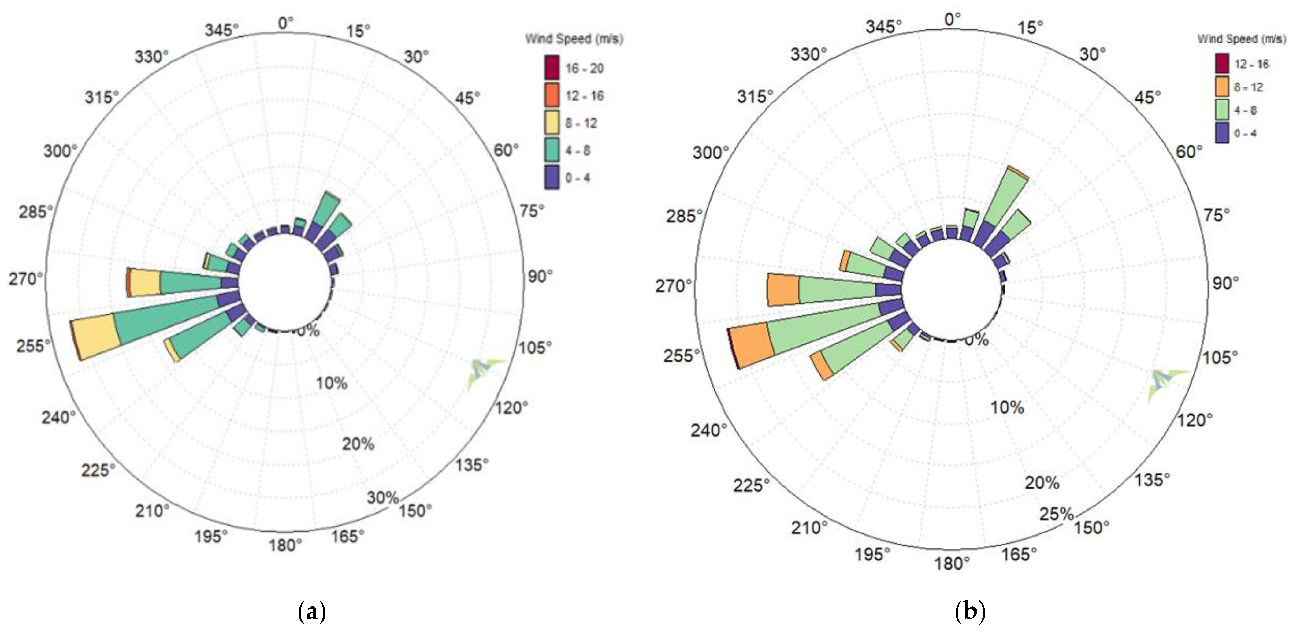
Figure 7 shows the wind rose diagrams for years 2016–2017 and 2017–2018. The Windographer software was used to obtain the wind rose diagrams for directional analysis of the available wind. In the figures, 0 degree represents north, and the whole is divided into 24 equal sectors. In the year 2016–2017, around 60% of wind exist in the sectors between 240 and 270 degrees clockwise, whereas 15 percent of the wind lies in the sectors between 30 and 45 degrees clockwise.

In the following year, 2017–2018, there is no significant change in the direction of the wind; around 55 percent wind lies in between 240 and 270 degrees, and almost 17 percent lies between 30 and 45 degrees clockwise. The maximum percentage of the wind lies in the south-west direction, which is ideal for wind turbines (WTs). Therefore, WTs are able to capture the maximum optimum power from the wind and work effectively, instead of changing the direction frequently.

4.4. Weibull Parameters Test Analysis

Table 2. Weibull paraments “k” and “c” at different heights for both years, 2016 to 2018.

Period	Height (m)	Methods
		PSO	CSO	GWO	EMJ	EPFM	MoM	MMLM
		k values
2016–2017	20	2.4198	2.4563	2.4078	2.3976	2.3461	2.388	2.3777
2017–2018		2.735	2.724	2.702	2.587	2.501	2.5788	2.5517
Overall		2.62	2.602	2.598	2.4827	2.4152	2.4737	2.4558
2016–2017	40	2.8019	2.8189	2.7979	2.7194	2.6379	2.7123	2.682
2017–2018		2.8758	2.8728	2.8718	2.917	2.7943	2.9117	2.8745
Overall		2.4583	2.4623	2.4563	2.8061	2.7061	2.7999	2.7637
2016–2017	60	3.161	3.138	3.117	2.8468	2.7665	2.8409	2.8298
2017–2018		3.2474	3.2764	3.2294	3.0246	2.9069	3.0204	3.0298
Overall		3.1992	3.1932	3.1622	2.9275	2.8302	2.9223	2.9167
2016–2017	80	3.0505	3.0795	3.0325	2.8732	2.8068	2.8675	2.8763
2017–2018		3.0385	3.0075	3.0065	3.0107	2.914	3.0064	3.0463
Overall		3.0707	3.0447	3.0287	2.9372	2.8567	2.9321	2.9527
		c (m/s) values
2016–2017	20	6.516	6.504	6.5	6.0512	6.0533	6.0516	6.0577
2017–2018		5.796	5.835	5.789	5.8681	5.8734	5.8686	5.8743
Overall		5.9	5.873	5.861	5.9606	5.9641	5.9611	5.967
2016–2017	40	7.0515	7.0565	7.0125	7.1178	7.125	7.1185	7.1148
2017–2018		6.7603	6.7413	6.7353	6.853	6.8647	6.8535	6.848
Overall		5.868	5.889	5.861	7.7218	7.7324	7.7224	7.7111
2016–2017	60	7.7415	7.7235	7.7125	7.8296	7.8381	7.8302	7.8194
2017–2018		7.4823	7.5283	7.4783	7.6122	7.6252	7.6126	7.6009
Overall		7.6866	7.6826	7.6586	6.9866	6.9958	6.9872	6.9826
2016–2017	80	8.1299	8.1769	8.1579	8.3321	8.3398	8.3328	8.3163
2017–2018		7.9597	7.9867	7.9407	8.1572	8.1687	8.1578	8.1438
Overall		8.1688	8.1918	8.1468	8.2452	8.2547	8.2458	8.2306

illustrated the Wb parameters “k” and “c” at different heights for both years (2016–2018) calculated using the seven methods. It is apparent from the table that the “k” ranged from 2.37 to 3.24, whereas the “c” ranged from 5.79 to 8.34 for the heights of 20 to 80 m. The shape parameter value increase with the increase in height, which indicates steady wind at the candidate site. The scale parameter for the two years was 7.1 m/s, which is almost the same as that for the two years independently. Fitness tests are used to compute the accuracy of the used methods. These tests also help us to compare different methods with each other. In this context, MBE, R², and RMSE errors are applied to the Weibull distribution curves and real data.

Table A1. Performance test results for Weibull fit.

Height (m)	Test	Method
		MMLM	EMJ	EPFM	MoM	GWO	PSO	CSO
20	MBE	−0.00997	0.01103	−0.07597	−0.06597	0.015103	−0.00804	−0.00144
	R2	0.96129	0.84516	0.98523	0.91523	0.991028	0.993437	0.994537
	RMSE	0.03155	0.01421	0.02007	0.04004	0.001153	0.001842	0.000158
40	MBE	−0.05597	−0.06297	0.00403	−0.06797	0.019703	−0.00364	−0.00604
	R2	0.96129	0.84516	0.98523	0.91523	0.994028	0.994137	0.994937
	RMSE	0.05845	0.00821	0.06793	0.05396	0.005253	0.004742	0.006642
60	MBE	−0.00897	−0.07497	−0.05097	−0.02097	0.012703	−0.00334	−0.00204
	R2	0.96129	0.84516	0.98523	0.91523	0.990328	0.991237	0.991137
	RMSE	0.04745	0.07021	0.02607	0.05296	0.001063	0.001042	0.000658
80	MBE	−0.05197	−0.07097	0.00903	−0.04897	0.018903	−0.00454	−0.00714
	R2	0.95365	0.96129	0.84516	0.98523	0.991523	0.996537	0.991937
	RMSE	0.05509	0.07999	0.06078	0.06961	0.000853	0.000642	0.000658
Accuracy %		95.9841	92.7189	95.9343	94.2539	99.1014	99.5627	99.5648

(see Appendix A) illustrates the fitness test results for different approaches. It shall be noted that all the used methods show acceptable fitness, suggesting the good fit of wind data with Weibull distribution. The accuracy percentage is also illustrated in Table A1. It shall be noted that although all the used methods show an acceptable accuracy, the accuracy percentage of all the AI methods is over 99%.

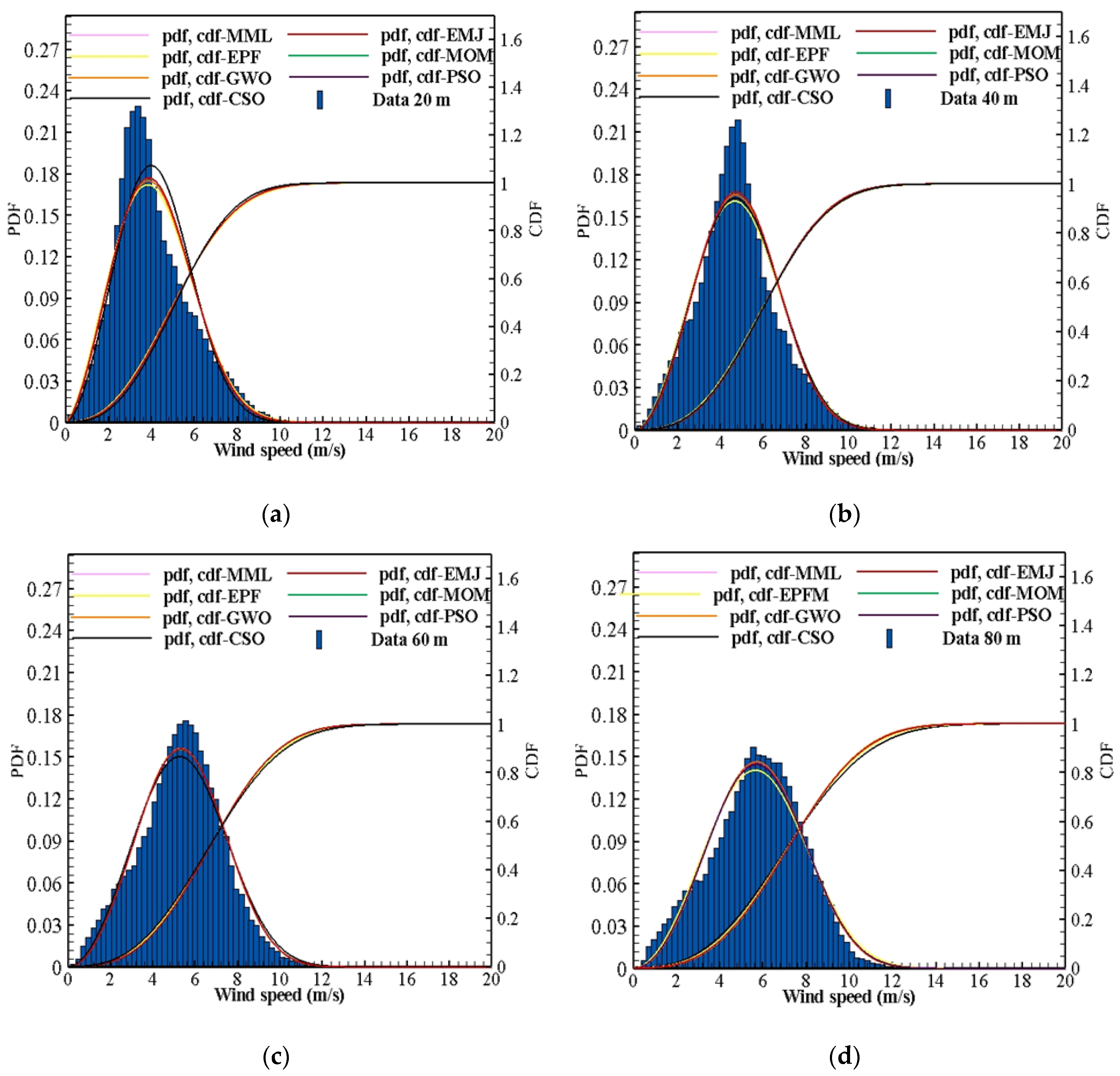
The good fit of these methods can also be seen in Figure 8a–d, where the probability density function and cumulative distribution for Weibull are presented at all mast heights for the year 2017–18. Moreover, the cumulative frequency for wind speeds more than 4 m/s was found to be 71%, 79%, 82%, and 85% at 20, 40, 60, and 80 m mast heights, respectively. It also exhibited that the probability for wind speed higher than 20 m/s is zero. The PDFs and CDFs for the year 2017–2018 at considered heights are depicted in Figure A1a–d.

It is challenging to analyze the fitness of distribution with multiple error functions. Therefore, a new fitness criterion is proposed based on the three error formulas. It is defined as

$$Net fitness=\frac{{{\displaystyle \sum }}_i^n\left|MB{E}_i\right|+{{\displaystyle \sum }}_i^{n}RMS{E}_i+{{\displaystyle \sum }}_i^n\left(1-R_i^2\right)}{3n}.$$

(26)

where n is the total number of error entries. Figure 9 presents the comparison of net fitness of the methods used for the estimation of Weibull parameters. It is apparent that all methods at all mast heights show acceptable performance. The error for AI algorithms ranges between 0.004276 and 0.005583, while that of the numerical methods ranges between 0.056606 to 0.067614. Figure 10 compares the convergence for all AI methods at the height of 80 m with 100 iterations. In both years, the grey wolf algorithm converges the fastest. However, all the methods perform similarly for the higher number of iterations.

4.5. Wind Energy Density and Specific Wind Characteristics

For the year 2016–2017, Weibull MWS, specific wind speeds, power density, and energy density at four heights are summarized in

Table 3. Weibull mean wind speed, specific wind speeds, power, and energy densities for the year 2016–2017.

Height (m)	Method	Vavg (m/s)	Vmp (m/s)	VmaxE (m/s)	PD (W/m2)	ED (kWh/m2)
80	EMJ	7.4268	7.1790	10.0140	346.6361	3036.5320
	EPFM	7.4268	7.1280	10.1020	351.5537	3079.6100
	MoM	7.4268	7.1750	10.0210	347.0417	3040.0850
	MMLM	7.4131	7.1690	9.9920	344.4921	3017.7500
	PSO	7.1401	7.0144	9.4259	344.8705	3021.066
	CSO	7.1584	7.0484	9.4198	345.0001	3022.201
	GWO	7.1275	6.9918	9.4282	346.9594	3039.364
60	EMJ	6.9763	6.7250	9.4390	288.8913	2530.6880
	EPFM	6.9763	6.6650	9.5410	293.9996	2575.4370
	MoM	6.9763	6.7210	9.4460	289.2523	2533.8500
	MMLM	6.9656	6.7030	9.4450	288.6086	2528.2120
	PSO	6.9296	6.8639	9.0402	288.0436	2523.262
	CSO	6.9111	6.8345	9.0376	288.3818	2526.225
	GWO	6.8991	6.8123	9.0419	289.7111	2537.869
40	EMJ	6.3313	6.0140	8.7170	222.1739	1946.2440
	EPFM	6.3313	5.9470	8.8250	226.6605	1985.5460
	MoM	6.3313	6.0080	8.7260	222.5454	1949.4980
	MMLM	6.3257	5.9790	8.7580	223.5748	1958.5150
	PSO	6.2792	6.0236	8.5464	223.3514	1956.559
	CSO	6.2851	6.0408	8.5349	224.078	1962.923
	GWO	6.2441	5.9872	8.5033	222.4333	1948.516
20	EMJ	5.3642	4.8310	7.7930	147.6697	1293.5860
	EPFM	5.3642	4.7770	7.8730	150.2098	1315.8380
	MoM	5.3642	4.8220	7.8080	148.1305	1297.6230
	MMLM	5.3692	4.8150	7.8310	149.0504	1305.6810
	PSO	5.7772	5.2275	8.3579	149.1503	1306.557
	CSO	5.7684	5.2572	8.2889	148.9265	1304.596
	GWO	5.7625	5.2013	8.3556	151.1166	1323.781

. The average wind speed ranged from 5.3 to 7.42 m/s, while V_mp and V_maxE are found between 4.7 to 7.2 m/s and 7.7 to 10.1 m/s, respectively. The annual Weibull PD and ED ranged between 147 to 351 W/m² and 1993 to 3079 kWh/m², respectively. The annual Weibull wind PD and ED, mean wind speed, and specific wind speeds for the year 2017–2018 are given in

Table A2. Weibull mean wind speed, specific wind speeds, power and energy densities for year 2017-2018.

Height (m)	Method	Vavg (m/s)	Vmp (m/s)	VmaxE (m/s)	PD (W/m2)	ED (kWh/m2)
80	EMJ	7.2854	7.134	9.661	318.187	2787.32
	EPFM	7.2854	7.071	9.773	324.119	2839.28
	MoM	7.2854	7.131	9.666	318.441	2789.54
	MMLM	7.2772	7.147	9.611	315.081	2760.11
	PSO	7.1119	6.9798	9.4012	351.639	3080.36
	CSO	7.1327	6.9823	9.4621	351.905	3082.69
	GWO	7.0916	6.9414	9.4086	353.442	3096.15
60	EMJ	6.8	6.666	9.003	258.075	2260.74
	EPFM	6.8	6.596	9.13	263.922	2311.96
	MoM	6.8	6.664	9.007	258.272	2262.47
	MMLM	6.7904	6.66	8.985	256.745	2249.09
	PSO	6.7064	6.6805	8.6739	256.686	2248.57
	CSO	6.7506	6.7364	8.7068	256.1	2243.43
	GWO	6.701	6.6676	8.6821	258.798	2267.07
40	EMJ	6.1122	5.934	8.196	191.285	1675.65
	EPFM	6.1122	5.858	8.328	196.259	1719.23
	MoM	6.1122	5.931	8.202	191.485	1677.4
	MMLM	6.1041	5.902	8.229	192.167	1683.38
	PSO	6.026	5.8269	8.1226	191.908	1681.11
	CSO	6.0088	5.8085	8.1025	192.762	1688.59
	GWO	6.0034	5.8026	8.0963	192.089	1682.7
20	EMJ	5.2113	4.858	7.322	127.93	1120.67
	EPFM	5.2113	4.789	7.429	131.032	1147.84
	MoM	5.2113	4.852	7.332	128.211	1123.13
	MMLM	5.2148	4.834	7.37	129.418	1133.7
	PSO	5.1566	4.9075	7.084	130.065	1139.37
	CSO	5.1906	4.933	7.142	131.007	1147.62
	GWO	5.1482	4.8788	7.1064	131.574	1152.59

.

According to wind power classes (WPC), regions that fall in WPC-III or above are suitable for most wind power conversion systems [19,49]. Results of measured wind speed and power density revealed that the Sujawal area stands in WPC-III and is suitable to harness the wind power.

4.6. Energy Production and Cost analysis

Total energy production and capacity factor are fundamental aspects of a wind power project. Furthermore, the capacity factor (CF) can be used to characterize the annual energy production (AEP) of the WTs. From [50], the random nature of wind usually affects the value of CF, which in result affects the efficiency and serviceability of the WTs. In practice, CF generally varies from 20% to 70%. The technical specifications of selected WTs are illustrated in

Table 4. Wind turbines (WTs) technical specifications.

WT Models	${\mathit{P}}_{\mathit{r}} \left(\mathbf{MW}\right)$	${\mathit{V}}_{\mathit{c}\mathit{i}} (\mathbf{m}/\mathbf{s})$	${\mathit{V}}_{\mathit{r}} (\mathbf{m}/\mathbf{s})$	${\mathit{V}}_{\mathit{c}\mathit{o}} (\mathbf{m}/\mathbf{s})$	Hub Height (m)	Diameter (m)
GE 1.7- 100	1.70	3	10	23	96	103
Nordex N90/2500	2.50	3	13.5	25	100	90
Vestas V80-2.0	2.00	4	15	25	100	80
Acciona AW-70/1500	1.50	4	11.6	25	80	70
Nordex N60/1300	1.30	2.5	15	25	60	60
Vestas V90-1.8	1.80	3.5	12	25	105	90
Enercon E-33/330	0.33	3	13	28	50	33.4
Enercon E-48/800	0.80	3	12	34	55	48
Suzlon S52-600	0.60	4	13	25	75	52
EWT DW54-500	0.50	2.5	10	25	40	54
GE 2.75-103	2.75	3	13	23	85	103
Gamesa g114-2.5	2.50	2	10	25	125	114
Windtec DF 2000 WT55	2.00	3	9.5	20	90	113
Siemens SWT-2.3-108	2.30	3	11.5	25	80	108

.

The energy produced is calculated using the WTs power curves data and the number of hours when the possibility of wind speed stayed in different bins at the turbine hub height; energy production, CF, and cost analysis are defined in [19,42,51]. The wind speed for different hub heights of the WTs is calculated using the power-law extrapolation model. The capacity factor (CF) and annual energy production (AEP) and of WTs with different power ratings ranged from 0.33 to 2.75 MW are estimated, respectively, and shown in

Table 5. WTs power production, annual energy production (AEP), capacity factor (CF), and cost/MWh.

WTs Model	Power (MW)	AEP (MWh)	CF	Cost$/MWh
GE 1.7- 100	0.8484	7432.23	0.474	22.72990001
Nordex N90/2500	0.863	7560.257	0.3452	31.21081287
Vestas V80-2.0	0.6089	5333.799	0.3044	35.39412813
Acciona AW-70/1500	0.4479	3923.376	0.2986	36.08162292
Nordex N60/1300	0.2571	2252.456	0.1978	54.46902226
Vestas V90-1.8	0.7084	6205.269	0.3935	27.37985414
Enercon E-33/330	0.0821	718.831	0.2487	43.32116045
Enercon E-48/800	0.1827	1600.826	0.2256	47.75697076
Suzlon S52-600	0.1963	1719.343	0.3271	32.93785571
EWT DW54-500	0.1627	1425.002	0.3253	33.12011252
GE 2.75-103	1.0917	9563.679	0.397	27.13847003
Gamesa G114-2.5	1.245	10905.966	0.498	21.63448314
Windtec DF 2000-WT55	1.0113	8858.846	0.5056	21.30928126
Siemens SWT-2.3-108	0.9814	8597.036	0.4267	25.24952567

. The calculations are made by assuming constant losses of 16.005%, i.e., turbine performance losses, wake effect losses, availability losses, and electrical losses.

The maximum AEP of 10905.966 MWh is gained by Gamesa G114-2.5 wind turbines followed by GE 2.75-103 (9563.679 MWh) and Windtec DF 2000-WT55 (8858.846 MWh). Whereas the minimum AEP of 718.831 MWh is generated by Enercon E-33/330, followed by EWT DW54-500 (1425.002 MWh). The CF is ranged between 0.20 to 0.51 for the selected WTs at their corresponding hub heights. The maximum CF is 0.51 for Gamesa G114-2.5, while minimum CF is 0.20 for Nordex N60/1300 wind turbine.

The estimated cost of energy per unit for WTs is given in Table 5. The cost of energy per unit is calculated by taking the assumptions (for instance, initial investment cost, operation and maintenance cost, real interest rate, life span, and cost of wind turbines) from the literature [19,42,51,52,53]. The lowest cost of energy (COE) per unit is 21.31 US Dollar $/MWh for Windtec DF 2000 followed by Gamesa G114-2.5 and GE 1.7- 100 with COE/unit 21.63 $/MWh and 22.72 $/MWh, respectively, while the highest COE is 54.47 $/MWh for Nordex N60/1300 followed by Enercon E-48/800 and Enercon E-33/330 with COE/unit 47.75 $/MWh and 43.32 $/MWh, respectively. Moreover, the cost of energy per unit ranges from 21.31 to 54.47 $/MWh. The capacity factor and cost/unit of all WTs are found in the appropriate range at the proposed site. Moreover, the capacity factor and cost/unit of selected WTs show that the Gamesa G114-2.5, Windtec DF 2000-WT55, and GE 1.7-100 wind turbines with the highest CF and lowest cost/unit are the most suitable for the selected site. Therefore, the WT models with corresponding specifications and power curves can be suitable for power production in the proposed area.

5. Conclusions

The Weibull distribution is considered as the most capable model for wind resource assessment in any region worldwide. Nevertheless, the precise estimation of its parameters remains a challenge for wind community researchers and developers. In this paper, a new criterion is introduced to estimate the Weibull parameters, which is based on the maximum distance metric. The proposed convergence objection function results are verified through mathematical expression. Furthermore, three artificial intelligence (AI) optimization algorithms are compared with four numerical methods using 2-year wind data (acquired from the Sujawal site). The goodness-fit tests show that the optimization algorithms have adequate accuracy for Weibull model parameter estimation in comparison to numerical methods.

The net fitness results for AI algorithms are ranged between 0.004276 and 0.005583, while that of the numerical methods ranged between 0.056606 to 0.067614. Furthermore, the average accuracy percentage of all the considered AI methods is over 99%. According to these findings, optimization algorithms present supremacy over numerical approaches. Also, the proposed convergent objective functions based on the maximum distance metric give a better approach for the optimization algorithms. The outcomes of the data analysis showed that the site has an energy density of about 3014.477 kWh/m², and a power density of 344.118 W/m² at the 80 m height.

The Windtec DF 2000-WT55 and Gamesa G114-2.5 wind turbines showed the highest annual energy production with good capacity factor and lowest cost of energy per unit, whereas, the capacity factor was found between 0.20 and 0.51 for the selected wind turbines. It is determined that the wind turbine models with corresponding specifications and power curves can be suitable for the investigated area. Besides, artificial intelligence optimization algorithms can be an alternative approach to the conventional numerical methods for Weibull model parameter estimation.