MIMR Criterion Application: Entropy Approach to Select the Optimal Quality Parameter Set Responsible for River Pollution

Abstract

Surface water quality has a vital role when defining the sustainability of the ecological environment, public health, and the social and economic development of whole countries. Unfortunately, the rapid growth of the worldwide population together with the current climate change have mostly determined fluvial pollution. Therefore, the employment of effective methodologies, able to rapidly and easily obtain reliable information on the quality of rivers, is becoming fundamental for an efficient use of the resource and for the implementation of mitigation measures and actions. The Water Quality Index (WQI) is among the most widely used methods to provide a clear and complete picture of the contamination status of a river stressed by point and diffuse sources of natural and anthropic origin, leading the policy makers and end-users towards a more and more correct and sustainable management of the water resource. The parameter choice is one of the most important and complex phases and recent statistical techniques do not seem to show great objectivity and accuracy in the identification of the real water quality status. The present paper offers a new approach, based on entropy theory and known as the Maximum Information Minimum Redundancy (MIMR) criterion, to define the optimal subset of chemical, physical, and biological parameters, describing the variation of the river quality level in space and time and thus identifying its pollution sources. An algorithm was implemented for the MIMR criterion and applied to a sample basin of Northeast Italy in order to verify its reliability and accuracy. A comparison with the Principal Component Analysis (PCA) showed how the MIMR is more suitable and objective to obtain the optimal quality parameters set, especially when the amount of investigated variables is small, and can thus be a useful tool for fast and low-cost water quality assessment in rivers.

1. Introduction

Rivers have a pivotal role in ecological and human health as well as in the economic development of territories, representing the main water supply for domestic use, irrigation, and industrial activities. In the last decades, their water quality has ever more worsened due to both natural processes and anthropic interventions, such as the discharge of industrial and municipal pollutants together with runoff from agricultural lands [1]. Recently, climate change has further contributed to increasing such problems in many countries, causing more and more extreme events. In fact, on the one hand, less inflow in rivers during draughts reduces the dilution of the contaminants introduced from human and natural sources; on the other hand, the more frequent occurrence of higher runoff due to intensive storms increases their load of pollutants. Similarly, the growth of water temperature modifies the bio-geo-chemical processes and reduces the dissolved oxygen concentration in natural channels, while the overflow of treated and untreated wastewater systems due to flooding seriously affects the biotic life cycle and the possibility of waterborne diseases [2]. In addition, the rapid growth of population and economic activities, together with the urban sprawl, are pushing towards a higher demand of high-quality water not often matched by the locally available resources, while the discharge of insufficiently treated wastewater raises expenses for downstream users and has damaging effects on the aquatic environments [2].

In this context, reliable information about river water quality must be collected for an efficient resource management and to implement protective measures and actions able to improve the conditions of the water bodies [3] as required by the Sustainable Development Goals (SDGs). Monitoring networks measuring various chemical, physical, and biological river quality parameters appear as a great source of information on the water status in space and time [4,5,6,7,8]. However, they do not provide a complete and clear picture of the scenario but only judgement in terms of individual parameters. In order to quickly and easily collect information on the river water quality with a global vision, different approaches based on the evaluation of only a few indices have been developed in recent years [9]. Among these, the Water Quality Index (WQI) method is widely used to simplify expressions of complex sets of pollution variables in rivers, lakes, and groundwater, and it is considered a key element in water resource management [10]. In particular, the WQI combines various environmental parameters and converts them into a unique value, detecting the overall status of water quality. Therefore, instead of comparing the different evaluation results of multiple parameters, the WQI method is a reliable approach able to provide integrated information on the quality [11]. Moreover, it helps decision makers to correctly and sustainably manage the water resource, it analyses the impacts of the application of regulatory policy or laws, and it provides a more comprehensive picture of the source’s quality for an easier understanding by non-technical stakeholders [12]. Introduced as early as 1965 by [13] to define the status of water quality in the Ohio River, it has undergone various formulations and modelling over time, becoming one of the 25 environmental performance indicators of the holistic Environmental Performance Index [14]. The evaluation of the WQI is based on four main steps: (1) choice of parameters; (2) calculation of sub-index values; (3) giving weights to the different parameters; (4) final assembly of the weighted sub-index values [15].

The parameters choice is one of the most important phases in the design of the WQI and also the most complex one. There are various WQIs across the world which are based on different selected parameters, ranging from 4 [16] to 26 [17]. In the last decades, most of the studies have focused on the design of a WQI with fewer environmental parameters able to describe the overall water quality, in order to reduce the repetitive or correlated environmental variables and lower the analytical and monitoring cost. Recently, various multivariate statistical techniques, including Cluster Analysis (CA), Principal Component Analysis (PCA), Factor Analysis (FA), and Discriminate Analysis (DA), have been widely used to select the few parameters able to detect variations in river water quality in space and time and to detect potential degradation sources within the basin. For instance, Kumarasamy et al. [18] investigated the hydrochemistry of the Tamiraparani river basin in Southern India with multivariate CA, PCA, and FA. Phung et al. [19] applied the CA, PCA, FA, and DA techniques to estimate the temporal and spatial changes of surface water quality in the Mekong Delta area of Vietnam. Correlation analysis, PCA, and CA components were employed by [20] to describe seasonal changes, identify contamination sources, and cluster monitoring stations of the Ganga and Yamuna rivers in the Uttarakhand State (India). In 2016, Barakat et al. [4] determined the main contamination sources in the Oum Er Rbia river and its main tributary in Morocco, using multivariate statistical methods including Pearson’s correlation, PCA, and CA. Zandagba et al. [21] studied the suitability of Nokoué’s water, one of the largest West African lagoons, and identified possible sources of pollution through Hierarchical Cluster Analysis (HCA) and PCA. Although such techniques are becoming more and more popular for their capacity to manage great volumes of spatial and temporal data deriving from a variety of gauge stations, they are still subjective because they depend on the number of parameters provided for the analysis [12,16].

The present paper offers a new approach on the basis of information theory, in order to select the variables causing the spatial and temporal quality variations of a river subject to point and diffuse pollution sources within basin. It provides powerful tools able to relate various interconnected flow data in order to obtain the best understanding of processes without any assumptions about the correlations/dependencies among time series. This theory, built on the mathematical concept of entropy, represents the quantitative measure of the information content associated with a signal. It has been widely used in different sectors of hydraulics and hydrology to derive models of rainfall-runoff, infiltration, and soil moisture [22,23,24,25,26,27] as well as distribution of velocity, sediment concentration, and shear stress in open-channel flows [28,29,30,31,32,33,34,35,36,37,38,39]. Among the different applications, information theory has also been employed for the optimization, design, and management of several gauge stations including networks of water quality and groundwater [40,41], rainfall [42,43], streamflow, and water level [44,45,46,47,48,49,50,51]. These problems can be solved through a multi-objective optimization approach, in which the repetitive information is minimized whilst the total information is maximized. This concept is known as Maximum Information Minimum Redundancy (MIMR) [45]. To the authors’ knowledge, the MIMR criterion has not yet been used for the identification of representative sets from an ensemble of quality parameters collected along a river. To that end, an easy-to-implement algorithm will be developed here and applied to a sample basin of Northeast Italy, subject to continuous stresses of urban and industrial origin, in order to verify its reliability and accuracy [52,53,54,55]. During the selection, the three norms of maximum overall information, maximum information transition ability, and minimum redundant information must be satisfied to achieve a unique solution under different scenarios with a good performance and to thereby simplify the decision-making process. The MIMR criterion, being based on a mathematical principle, could be more objective and less affected by the number of investigated variables compared to other selection methods. In fact, the above-mentioned four most used techniques for parameter selection (CA, PCA, FA, and DA) are characterized by several disadvantages: the need of correlated parameters; the strict assumption about their relation having to be linear, which occurs very rarely; and the required number of over 300 measured data points [56,57] for the investigated sample, in order to obtain reliable results. The MIMR approach, instead, would allow identifying only the parameters mostly responsible for the river pollution. In this way, the local monitoring programs could be better addressed and prioritized, increasing both the recording frequency of these parameters and the amount of measuring sites, especially in fluvial reaches at higher risk of contamination and located in strongly anthropized, industrial, and agricultural areas. A fast and simplified water quality assessment, based on few parameters, could thus be more easily communicated and better understood by the public and non-technical stakeholders. In addition, the local administrators and policy makers could be guided towards a faster and better choice of mitigation measures and structural investments in order to achieve some of the Sustainable Development Goals (SDGs) such as:

-

the significant reduction of pollutants in fluvial and marine environments (Goals 6.3 and 14.1);

-

the minimum release of hazardous substances and of untreated wastewater in rivers (Goal 6.3);

-

an increasingly efficient and right use of the water resource (Goal 12.2);

-

cleaner water to satisfy the needs of society and the safe use of surface waters for recreational purposes, hygiene, and household activities (Goal 6.4).

The paper is organized as follows: in Section 2, the study area and data are introduced, the basic entropy theory is briefly described for an easier understanding of the MIMR criterion, and the selection algorithm is presented; Section 3 reports the results of the MIMR application in the identification of the representative quality parameters set, the potentialities of the proposed framework, and the comparison with the PCA selection method; finally, Section 4 states the conclusions.

2. Materials and Methods

2.1. Study Area and Data Collection

The Bacchiglione basin, located in Northeast Italy, covers a surface of about 1177 km² with broad-leaved and coniferous forests dominating the mountainous area and non-irrigated arable land, together with small and discontinuous urban fabric and concentrated industrial and commercial sites in the remaining part up to the mouth (Figure 1). The Bacchiglione river has a length of 119 km, originates from Dueville springs, and crosses two major cities, Vicenza and Padova, flowing into the Adriatic Sea. The main channel is characterized by the presence of gravel boulders, cobbles, and aquatic plants on the bottom while cane fields and shrubbery cover the banks. The fauna is especially linked to the flora and the most common type is ornithofauna (native fauna), and the species most easily observed are moorhens and glens. In the mountain area, the water discharge trend shows a significant variability all year round, with high values in the winter months and low values in summer months. The flow rate decreases going along the river due to the increasing agricultural water demand, and only near the big cities an increase is recorded because of urban and industrial wastewaters. The most important causes of water quality contamination in the Bacchiglione basin are to be found in the high population density and the presence of tourists all year round, together with the numerous industrial settlements.

Six quality parameters—Dissolved Oxygen (DO), five-day test for Biochemical Oxygen Demand (BOD₅), Ammonia Nitrogen (NH₄-N), Nitrate Nitrogen (NO₃-N), Total Phosphorus (TP), and Escherichia Coli (E. coli)—were analyzed through the MIMR criterion to select the variables set responsible for the river contamination level. They were sampled with 720 data points for each parameter from January 2008 to December 2017 at 12 gauge stations by the Regional Environmental Prevention and Protection Agency of Veneto (ARPAV), according to the National Environmental Quality Standards for Surface Water (Legislative Decree No. 152/2006). The gauge stations were chosen because, in addition to being distributed along the main reach of the river, they also measured both the flow depth and quality parameters (Figure 2). All stations usually acquired data with a quarterly frequency (40 data points per site and parameter), excluding stations 326, 174, and 181 which, addressing drinking water purification, recorded with a monthly frequency (120 data points per site and parameter).

2.2. Basic Entropy Measures

Shannon [58] developed the concept of entropy as a measure of information, disorder, chaos, or uncertainty. Considering a certain event, defined as a discrete random variable X, it can occur in different ways and lead to different outcomes, X₁, X₂,…, X_N, with probabilities p(X₁), p(X₂),…, p(X_N), respectively. Therefore, the probability of occurrence, p(X_i), of the event X_i can thus be interpreted as a measure of uncertainty about the occurrence of the event X_i and also provides an evaluation of the event information content. When an event occurs with high probability, less information will be needed to characterize the event. On the other hand, more information will be needed to characterize the event if it occurs with low probability, p(X_i). This means that a more uncertain event transmits more information or that more information is required to characterize it. Subsequently, being a measure of the amount of uncertainty, entropy represents the information content of the event or its probability of occurrence. Since the information content of an event, X_i, can be expressed as the logarithm of its occurrence probability, p(X_i), entropy H(X) can thus be quantitatively defined as the probability-weighted average of the information content of each event X_i:

$$H\left(X\right)=-{{\displaystyle \sum }}_{i=1}^{N}p(X_i)lo{g}_2\left[p\left(X_i\right)\right].$$

(1)

H(X) is measured in average number of binary digits (bits) and takes values between 0 (complete information) and log₂N (no information).

In the case of an ensemble of multivariate discrete random variables N, the joint entropy can be described as a measure of the overall information of the random variables, i.e.,

$$H\left(X_i,\dots ,X_N\right)=-{{\displaystyle \sum }}_{i_1=1}^{N_1}\dots {{\displaystyle \sum }}_{i_N=1}^{N_N}p\left(X_1,\dots ,X_N\right)·lo{g}_{2}p\left(X_1,\dots ,X_N\right),$$

(2)

where p(X₁,…, X_N) is the joint probability of the N variables. When the random variables are stochastically independent, the joint entropy is equal to the sum of its one-dimensional marginal entropies; otherwise, it is smaller.

It is probable that the information regarding one random variable (e.g., X₁) can be derived from knowledge of another variable (e.g., X₂) of the same ensemble. Mutual information, also known as transinformation, measures the linear or nonlinear dependence between two random variables and detects how much uncertainty can be reduced in one of the variables when the other variable is equal to the difference between the total entropy and the sum of the single entropies. For more than two variables, the multidimensional transinformation between the n existing parameters and the new (added) parameter (n+1) can be defined as:

$$T\left[\left(X_1,X_2,\dots ,X_n\right),X_{n+1}\right]=H\left(X_1,X_2,\dots ,X_n\right)-H\left[\left(X_1,X_2,\dots ,X_n\right),X_{n+1}\right].$$

(3)

The transinformation is between 0 and H(X). It is zero when the variables are statistically independent, while it is equal to H(X) when the variables are functionally dependent and, thus, the information at one parameter can be fully transmitted to another parameter with no loss of information at all. Larger values of T correspond to greater amounts of information transferred. To assess the redundancy and the amount of duplicated information in a set of parameters, the total correlation can be calculated, and its mathematical expression is equal to:

$$C\left(X_1,\dots ,X_N\right)={{\displaystyle \sum }}_{i=1}^{N}H\left(X_i\right)-H(X_1,\dots ,X_N),$$

(4)

where H(X_i) is the marginal entropy of the ith random variable and H(X₁,…, X_N) is the joint entropy of the N random variables. It is equal to 0 when all random variables are independent, otherwise H(X₁,…, X_N) > 0.

2.3. MIMR Criterion

The main concept of the MIMR approach is to choose a parameter set able to: (1) maximize the whole information content (joint information), (2) maximize the entire information transition ability (transinformation), and (3) minimize the redundant information (total correlation) [45].

Let there be N potential candidate parameters monitored in the gauge stations located along the river. For each candidate parameter, there are some years of records denoted by X₁, X₂, X₃,…, X_N. Let S be the set of parameters already selected and its elements represented by X_S1, X_S2,…, X_Sk. Similarly, let F be the set of candidate parameters to be selected and its elements denoted as X_F1, X_F2, X_F3,…, X_Fm. The sum of k and m is the total number, N, of potential candidate parameters. The effective information of S can be modelled as joint entropy and transinformation:

$$H\left(X_{S1},X_{S2},\dots ,X_{Sk}\right)+{{\displaystyle \sum }}_{i=1}^{m}T\left(X_{S1:Sk};X_{Fi}\right),$$

(5)

or

$$H\left(X_{S1},X_{S2},\dots ,X_{Sk}\right)+{{\displaystyle \sum }}_{i=1}^{m}T\left(X_{S1:Sk};X_{Fi:F_m}\right),$$

(6)

where X_S1:Sk is the merged time series of X_S1, X_S2, X_S3,…, X_Sk, and its marginal entropy is equal to the multivariate joint entropy of X_S1, X_S2, X_S3,…, X_Sk. In particular, the first part of the equation is the joint entropy, measuring the total but not duplicated amount of information, which can be obtained from the selected parameters. The second part is the information transition ability of S, which can be measured by the sum of the transinformation between grouped variables in S and each parameter in F (Equation (5)) or between grouped variables in S and in F (Equation (6)).

Another key point to consider is the redundant information among the selected parameters, and it can be measured from the total correlation as:

$$C\left(X_{S1},X_{S2},\dots ,X_{Sk}\right),$$

(7)

Therefore, the MIMR criterion-based objective functions is formulated as:

$$max: H\left(X_{S1},X_{S2},\dots ,X_{Sk}\right)+{{\displaystyle \sum }}_{i=1}^{m}T\left(X_{S1:Sk};X_{Fi}\right),$$

(8)

$$min: C\left(X_{S1},X_{S2},\dots ,X_{Sk}\right),$$

(9)

or

$$max: H\left(X_{S1},X_{S2},\dots ,X_{SK}\right)+{{\displaystyle \sum }}_{i=1}^{m}T\left(X_{S1-Sk};X_{Fi:Fm}\right),$$

(10)

$$min: C\left(X_{S1};X_{S2},\dots ,X_{Sk}\right),$$

(11)

This constitutes a multi-objective optimization problem, which can be unified to a single objective optimization problem through integrated functions in order to facilitate the end-user’s decision making:

$$max: {\lambda }_1(H\left(X_{S1},X_{S2},\dots ,X_{Sk}\right)+{{\displaystyle \sum }}_{i=1}^{m}T(<X_{S1},X_{S2},\dots ,X_{Sk}>;X_{Fi}))-{\lambda }_{2}C\left(X_{S1},X_{S2},\dots ,X_{Sk}\right),$$

(12)

$$max: {\lambda }_1(H\left(X_{S1},X_{S2},\dots ,X_{Sk}\right)+{{\displaystyle \sum }}_{i=1}^{m}T(<X_{S1},X_{S2},\dots ,X_{Sk}>;<X_{Fi},\dots ,X_{Fm}>))-{\lambda }_{2}C\left(X_{S1},X_{S2},\dots ,X_{Sk}\right)$$

(13)

where λ₁ and λ₂ are the information and redundancy weights, respectively, and their sum is 1. Their variations allow users to obtain different possible solutions under various scenarios. Since the first goal is the maximum information of the parameter set, λ₁ should be usually larger than λ₂ [45]. A sensitivity analysis on different information redundancy weights found that most parameters kept stable with λ₁ between 0.5 and 1 and λ₂ between 0.5 and 0.

2.4. Selection Procedure

The application of MIMR criterion requires a selection procedure, which presents the following steps:

• collecting the continuous time series of each potential candidate parameter and discretizing them;
• calculating marginal entropies for all the candidate parameters;
• identifying the parameter with the maximum marginal entropy and defining it as the main parameter;
• updating the S set, where the parameters already selected are saved, and the F set, where all the unselected candidate parameters are saved;
• selecting the next parameter from the F set by the MIMR criterion. In this step, all parameters in F are scanned sequentially to search the one satisfying Equation (10) or Equation (11);
• repeating steps 4 and 5 until the expected number of parameters is selected.

The convergence of the selection depends on the ratio between the joint entropy of the selected parameters and of all potential candidate parameters. These steps show that if no convergence threshold is provided, then all potential candidate parameters will be ranked in descending order, which will help to determine the parameter with the least degree of importance. An algorithm in MATLAB was built in order to minimize the implementation effort.

2.5. Data Discretization

The continuous time series acquired at the gauge stations along the river should be discretized in order to know the entropy terms. Various approaches exist for data discretization, such as the histogram method and the mathematical floor function. For the application of histogram discretization, an arbitrary number of bins must be assumed, which is a questionable method since entropy terms depend on the bin size. In particular, the entropy values decrease as the bin width increases. The subjective calculation of the bin size could be overcome with the use of a mathematical floor function which converts a continuous value x in its nearest and lowest integer multiple of a constant a, i.e.,

$$X_q=a\left[\frac{2x+a}{2a}\right],$$

(14)

where [·] is the mathematical floor function, X_q the quantized discrete value, and a the bin width. The advantages of the mathematical floor function are the lack of a parametric distribution and the inclusion of physical considerations where the resolution of a should not be less than the uncertainties involved in the continuous data. However, determining an appropriate a is not always easy, and the selection of a should guarantee that: (a) all candidate parameters have significant and distinct information; (b) the spatial and temporal variability of time series is preserved before and after discretization as much as possible; and (c) the selected parameters are as stable as possible, when a varies within an interval near its optimal value. In this paper, the bin width was calculated through known empirical formulas of [59,60,61]. Scott [59] proposed an optimal bin width as:

$$a=3.49\sigma \left(x\right)N^{-\frac{1}{3}},$$

(15)

where σ is the standard deviation of an observation series of X and N is the sampling size.

Sturges [60] estimated the bin width as:

$$a=\frac{R_x}{1+lo{g}_{2}N},$$

(16)

where R_x represents the range of X and N its sampling size.

Bendat and Piersol [61] suggested another method for defining an optimal bin width:

$$a=\frac{R_x}{1.87{\left(N-1\right)}^{0.4}},$$

(17)

where R_x is the range of X and N its sampling.

3. Results and Discussion

3.1. Entropy Evaluation and Data Length Effect

The entropy values, reported in

Table 1. Entropy values with different bin widths.

Binning Evaluation	Maximum Marginal Entropy	Average Marginal Entropy	Joint Entropy	Total Correlation
Scott	2.86	1.46	5.78	2.96
Sturges	2.39	1.23	7.31	1.97
Bendat and Piersol	2.55	1.41	5.55	2.91

, are only slightly affected by the different bin widths calculated by the methods of Scott, Sturges, and Bendat and Piersol described in the previous paragraph. The maximum and average marginal entropies evaluated through Sturges’ approach are a little lower than the others. All three methods present joint entropies lower than the saturated value which is equal to log₂(n) = 9.49 bits (where n is the number of data acquired in ten-year observation equal to 720). Although there are no significant differences among the three methods, Sturges’ formula seems to show the highest information content and lowest redundancy of the time series. Considering the seasonal trend, the entropy values tend to level out, reducing even more the differences among the three methods (

Table 2. Seasonal entropy values with different bin widths.

Binning Evaluation	Season	Maximum Marginal Entropy	Average Marginal Entropy	Joint Entropy	Total Correlation
Scott	winter	2.36	1.31	6.63	0.52
	spring	2.21	1.30	6.45	1.35
	summer	2.27	1.19	6.43	1.26
	autumn	2.25	1.25	6.49	0.99
Sturges	winter	2.25	1.09	6.55	0.10
	spring	2.13	1.26	6.27	1.26
	summer	2.23	1.11	6.47	0.15
	autumn	1.99	1.08	6.37	0.25
Bendat and Piersol	winter	2.32	1.27	6.75	0.56
	spring	2.21	1.40	6.68	1.75
	summer	2.16	1.23	6.62	0.89
	autumn	2.24	1.27	6.64	0.96

).

However, a slight increase in the winter months is still detectable compared to the rest of the year, which could be explained reporting the seasonal trend of each single parameter (Figure 3). The box-plots were built gathering the data of all gauge stations along the river. In particular, as shown by the figure, the mean and standard deviation values of E. coli concentrations are significantly higher in winter than those measured in other seasons, due to domestic and industrial discharges. The seasonal DO content depends on the water temperature (T) which mainly affects the solubility of oxygen. In fact, it increases during winter, when T is lower, and vice versa in the summer. The lowest mean concentrations of NH₄-N occur in summer for excessive fertilizer use on agricultural land, while the mean concentration of NO₃-N is maintained roughly constant for the whole year. The same behavior is observed for TP, even though the standard deviations are slightly higher in hot seasons, while the BOD₅ parameter shows a high concentration especially in winter due to the presence of a large discharge of urban and industrial wastewaters in the river. In summary, the higher values of mean concentrations and their standard deviation for most parameters confirm the increase of the information content detected in winter months.

With regard to the joint entropy, the values obtained from Scott’s and Bendat and Piersol’s formulas increase, while Sturges’ decreases, reducing their distance. This underlines that, in the investigated case, the estimation method of the bin width does not particularly influence the entropy values, and thus, any formula could be chosen for the data discretization.

The maximum and average marginal entropies, the joint entropy, and the total correlation of time series were calculated by increasing their length in order to know the influence of the data length on the values of entropy terms. Figure 4 demonstrates how the temporal trends are very similar for the three methods of binning evaluation. The values usually become higher with increasing data length and then tend to stabilize. The trends are not monotonous, and fluctuations are evident at certain data lengths (e.g., around 1 year, 3 year, and 5 year) according to previous studies [62,63]. Moreover, it is interesting to note how the entropy values, estimated using 1-year, 2-year, and 5-year series, nearly reach 60%, 75%, and 90% of the ones calculated in 10 years of data. More importantly, as the measure parameters are subject to variability among years due mainly to different meteorological conditions, it is necessary to detect and estimate such variability with shorter time series. Although, in this paper, the quality parameters observed in at least 10 years were used for the MIMR selection, shorter lengths of series (1-year, 2-year, and 5-year) could also be considered, especially when a limited amount of data is available.

3.2. Application of MIMR Criterion

The MIMR criterion was applied according to the procedure described in Section 2.4, and a threshold of 0.95 was chosen in order to consider 95% of the total joint entropy in the data set and thus obtain the optimal subset of parameters.

With regard to the values of λ₁ and λ₂, the main purpose of the analysis is to obtain the maximum information from the selected parameters, and thus the first one needs to be higher than the second one, as suggested by [45]. Therefore, a sensitivity analysis was carried out varying λ₁ from 0.5 to 1 and λ₂ from 0.5 to 0 (

Table 3. Sensitivity analysis of the selected parameters with varying information weights.

Binning Evaluation		Iteration Step
	λ1	1	2	3	4	5	6
Scott	0.5	DO	E. coli	NH4-N	NO3-N	TP	BOD5
	0.6	DO	E. coli	NH4-N	NO3-N	TP	BOD5
	0.7	DO	E. coli	NH4-N	NO3-N	TP	BOD5
	0.8	DO	E. coli	TP	NH4-N	BOD5	NO3-N
	0.9	DO	E. coli	TP	NH4-N	BOD5	NO3-N
	1.0	DO	E. coli	TP	NH4-N	BOD5	NO3-N
Sturges	0.5	DO	E. coli	NO3-N	NH4-N	TP	BOD5
	0.6	DO	E. coli	NO3-N	NH4-N	TP	BOD5
	0.7	DO	E. coli	NO3-N	NH4-N	TP	BOD5
	0.8	DO	E. coli	TP	NH4-N	BOD5	NO3-N
	0.9	DO	E. coli	TP	NH4-N	BOD5	NO3-N
	1.0	DO	E. coli	TP	NH4-N	BOD5	NO3-N
Bendat and Piersol	0.5	DO	E. coli	NH4-N	NO3-N	TP	BOD5
	0.6	DO	E. coli	NH4-N	NO3-N	TP	BOD5
	0.7	DO	E. coli	NH4-N	NO3-N	TP	BOD5
	0.8	DO	E. coli	TP	NH4-N	BOD5	NO3-N
	0.9	DO	E. coli	TP	NH4-N	BOD5	NO3-N
	1.0	DO	E. coli	TP	NH4-N	BOD5	NO3-N

). The results of Table 3 show the stability of MIMR with increasing values assigned to the information weights. In the present case, such stability is especially guaranteed from the small number of data. In fact, the correct choice of values of λ₁ and λ₂ is based on a deep knowledge of the system, which it is not always possible. Selecting optimal weights still represents a challenge, and thus investigating the performance of MIMR with different values of λ₁ and λ₂ can provide useful suggestions. In particular, by increasing the value of λ₁, a more informative but less independent parameter set is derived. As seen from Figure 5, Figure 6 and Figure 7, a value of 0.8 for information weight leads to a good balance between information and redundancy. To sum up, the values of λ₁ = 0.8, λ₂ = 0.2, and a threshold of 95% were used in this study.

Table 4. Maximum Information Minimum Redundancy (MIMR) results over the entire 10-year series.

		Winter	Spring	Summer	Autumn
Scott	Set of selected parameters	DO, E. coli	DO, E. coli	DO, E. coli	DO, E. coli
	Joint Entropy	4.51	4.52	4.27	4.35
	Information Transition Ability	6.91	6.37	6.85	6.59
	Total Correlation	0.42	0.41	0.42	0.47
	MIMR value	10.43	9.91	10.19	9.97
Sturges	Set of selected parameters	DO, E. coli	DO, E. coli	DO, E. coli	DO, E. coli
	Joint Entropy	2.49	2.41	2.27	2.41
	Information Transition Ability	7.01	6.78	6.72	6.90
	Total Correlation	0.011	0.012	0.013	0.013
	MIMR value	9.00	8.70	8.53	8.82
Bendat and Piersol	Set of selected parameters	DO, E. coli	DO, E. coli	DO, E. coli	DO, E. coli
	Joint Entropy	4.20	4.16	3.99	3.71
	Information Transition Ability	6.93	6.63	6.75	6.94
	Total Correlation	0.035	0.038	0.040	0.034
	MIMR value	10.29	9.95	9.93	9.91

reports the results of the MIMR criterion application over the entire 10-year series. As highlighted in the table, the optimal representative subset of selected parameters, characterized by a balance among maximum total information, maximum transition ability, and minimum redundant information, is constituted by Dissolved Oxygen and Escherichia Coli, and it stays constant under different time windows and seasonal conditions. In this way, the MIMR criterion could be used to simplify and speed up the analysis process which leads to the quality assessment of the Bacchiglione river. In particular, the correlation between the temporal and spatial variability of only two parameters with one of the different factors affecting the water quality, such as population growth, climate change, uncontrolled tourism, numerous industrial settlements, and excessive land exploitation, allows to rapidly identify the point and/or diffuse pollution sources within the basin. For example, Escherichia Coli is an indicator of a fecal contamination probably due to the discharge of untreated municipal wastewaters into the river and surface runoff of pastures and fields used for livestock farming. At the same time, the reduction of Dissolved Oxygen could be associated to the release of untreated domestic sewages when the fluvial reach flows through strongly urbanized areas or to the release of fertilizers and pesticides when it crosses intensive agricultural lands.

3.3. Comparison with PCA

The performance of the MIMR criterion was compared with another method, i.e., Principal Component Analysis, which is now the most used multivariate statistical approach able to detect relationships between the water quality parameters, define contamination sources, and group gauge stations with similar characteristics into clusters. The application of PCA was preceded by a data standardization consisting of computing the z-score values of the parameters, which have zero mean and unit variance, in order to reduce the impact of difference on the variance of variables, balance the variable sizes, and make the measurement units uniform. The appropriateness of the dataset for the PCA was verified through the Kaiser–Meyer–Olkin (KMO) and Bartlett’s tests of Sphericity. The KMO index measures the sampling suitability that represents the variance caused by underlying principal components. In particular, if this index is greater than 0.5, the factor analysis is satisfactory. In the present case, the KMO had a value of 0.68. Bartlett’s test of Sphericity, instead, checks if variables are related; that is, the correlation matrix is an identity matrix, making PCA an unsuitable technique for the data analysis. In the present case, the correlation matrix is not an identity matrix, therefore PCA can be both applied efficiently on all data and grouped by season in order to define interrelationship among the parameters. The results of the PCA obtained using the SPSS Software are shown in Figure 8 and

Table 5. Loadings values for water quality parameters in all seasons.

	PCA1	PCA2
E. coli	0.781	0.022
NH4-N	0.565	0.428
NO3-N	0.061	0.684
TP	0.774	−0.230
BOD5	0.634	0.375
DO	−0.016	0.752

and

Table 6. Loading values for water quality parameters in (a) winter, (b) spring, (c) summer, and (d) autumn.

	PCA1	PCA2		PCA1	PCA2
E. coli	0.744	−0.264	E. coli	0.761	−0.213
NH4−N	0.574	0.362	NH4−N	0.636	−0.353
NO3−N	−0.138	−0.354	NO3−N	0.154	0.44
TP	0.788	−0.186	TP	0.588	0.243
BOD5	0.709	0.323	BOD5	0.75	0.349
DO	−0.172	0.831	DO	−0.109	0.788
(a)			(b)
	PCA1	PCA2		PCA1	PCA2	PCA3
E. coli	0.751	0.123	E. coli	0.851	−0.086	0.017
NH4−N	0.743	−0.273	NH4−N	0.444	0.660	0.052
NO3−N	0.423	−0.430	NO3−N	−0.194	0.898	−0.042
TP	0.706	0.145	TP	0.790	0.095	−0.099
BOD5	0.614	0.116	BOD5	0.483	0.361	0.465
DO	0.135	0.878	DO	−0.12	−0.066	0.933
(c)			(d)

.

In this study, the two principal components, which have eigenvalues >1 and explain almost 56% of the total variance in the water dataset, were retained. In autumn, the third component also appears with an eigenvalue slightly greater than 1. The variables with eigenvalues <1 were eliminated due to their low significance [64]. The PC loadings with values >0.75, 0.75–0.50, and 0.50–0.30 were classified as strong, moderate, and weak, respectively [65]. The first factor (PC1), accounting for the 35% of the total variance, shows strong positive loadings of E. coli and TP, and moderate positive loading of NH₄-N and BOD₅. If one considers the seasonal variation, the situation is very similar with 34%, 32%, 36%, and 33% in winter, spring, summer, and autumn, respectively. The parameter E. coli remains constantly high for the whole year, while TP decreases in spring. NH₄-N furtherly increases in summer and BOD₅ shows lower values in autumn. The second factor (PC2) explains 56% of the total variance and has a strong positive loading on DO and positive moderate loading on NO₃-N. While the oxygen remains high all year round, the NO₃-N levels are quite low if one considers the seasonal trend. According to the PCA, the identified parameters are four, and they become more or less significant in the different seasons. The MIMR criterion, instead, provides only two parameters, Dissolved Oxygen and Escherichia Coli, which stay constant under different meteorological conditions. This result underlines how this method seems to be more suitable to detect the optimal parameters set both when the amount of the investigated variables is small and when a non-linear relationship among parameters exists, being the MIMR criterion independent from the correlations among time series.

4. Conclusions

The rapid growth of the worldwide population, together with the current climate change, are contributing to the increase of river pollution, pushing research towards the development and implementation of effective methodologies able to rapidly and easily provide reliable information on the degradation status.

The Water Quality Index (WQI) proved to be a useful tool to obtain a clear and complete picture of the contamination level of a river stressed by point and diffuse sources of natural and anthropic origin, leading the policy makers and end-users towards a more and more correct and sustainable management of the water resource. Such index is often based on a significant number of environmental parameters describing the overall water quality and, recently, most of the studies have focused on reducing them in order to remove the redundant variables and lower the analytical and monitoring costs. Therefore, the quality parameters selection represents one of the most important and complex phases for the design of the WQI, and recent multivariate statistical techniques do not seem to show great objectivity and accuracy in the identification of the real water pollution status.

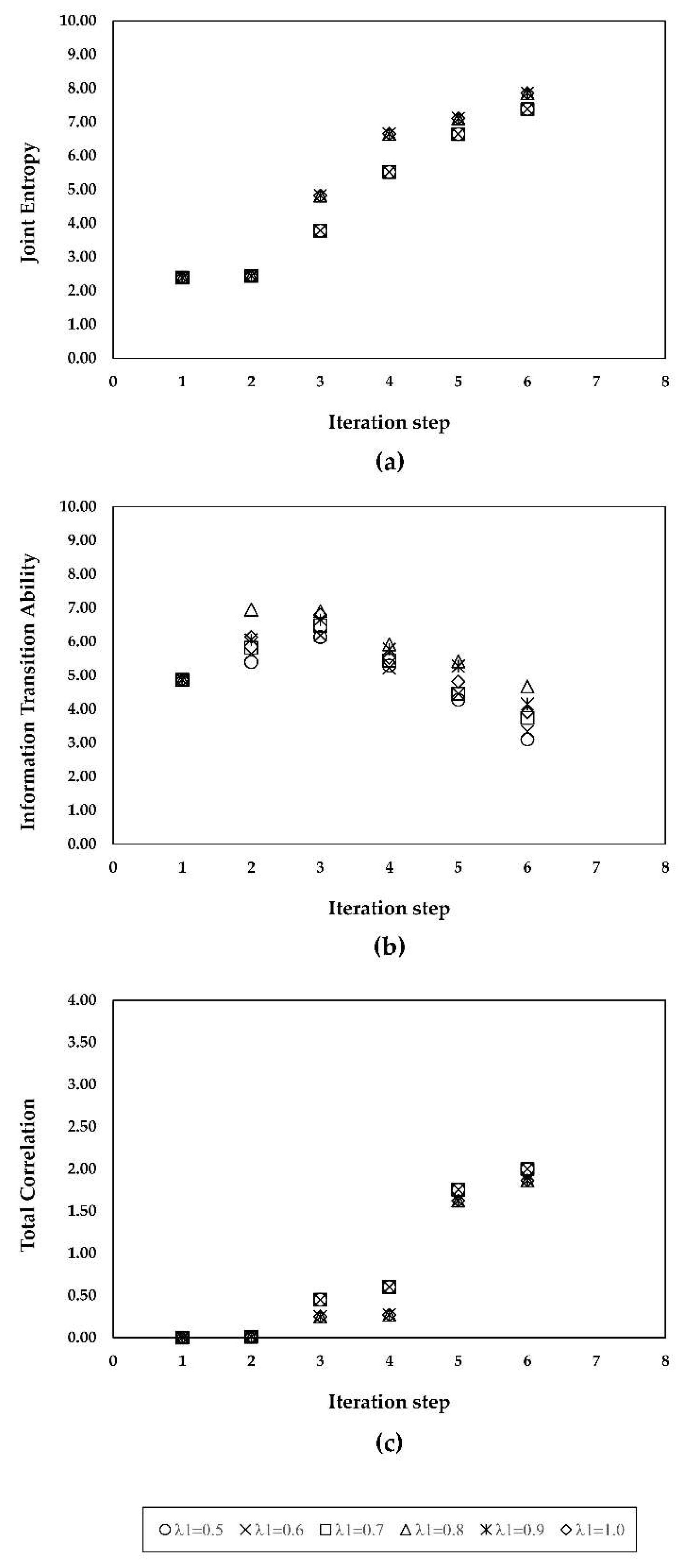
This study proposes a new method based on information theory in order to select the variables causing the quality variations in time and space of a river subject to point and diffuse pollution sources within the basin. Such method, known as the Maximum Information Minimum Redundancy (MIMR) criterion, built on the mathematical concept of entropy, allows choosing the parameters through a multi-objective optimization approach, where the repetitive information is minimized whilst the total information is maximized. The criterion was validated on a sample basin of Northeast Italy subject to continuous stresses of urban and industrial origin. Its application required the data discretization using a mathematical floor function, which converts continuous random variables to integers assigning a proper value of the bin width. In the present paper, the three known empirical formulas, used to define the optimal bin width, showed not to significantly affect the entropy values, leading to the conclusion that any formula could be chosen for the data discretization. The assessment of the quality parameters’ information content under different time windows highlighted its reaching about 90 % in 5-years, compared to the one calculated in 10 years, demonstrating how shorter lengths of series could also be considered, especially when a limited amount of data is available. Besides, a sensitivity analysis, performed by varying the information redundancy tradeoff weights, allowed choosing the most suitable weights to balance the two conflicting objectives, maximum information and minimum redundancy, and thus obtaining the optimal representative subset of quality parameters.

The MIMR criterion was also quantitatively compared to the multivariate statistical approach PCA, and the results showed how the MIMR seems be more suitable to detect the optimal parameters set both when the amount of the investigated data is small and when a non-linear relationship among the parameters exists. In fact, this set of parameters, constituted by Dissolved Oxygen and Escherichia Coli, stays constant both when considering all data and when grouping them in the four seasons. This way, the MIMR criterion could be used to develop a future WQI, more objective and more correctly weighted, able to provide a better water quality assessment of the Bacchiglione river under different conditions. In addition, the correlation between the spatial and temporal variability of only two parameters and one of the factors affecting the river quality status also allows a faster and clearer identification of the contamination sources within the basin. This can help the environmental managers to better address and prioritize the local monitoring activities and guide the local administrators and policy makers towards the choice of mitigation measures and structural investments, which could speed up the achievement of the Sustainable Development Goals (SDGs). Some of these mitigation measures and interventions could be the adoption of good land use practices and sustainable food production systems (Goal 2.4), the re-naturalization of some fluvial reaches with parks and green areas (Goal 6.6), the revamping of wastewater treatment plants with advanced technologies (Goal 6.A), and the building of new treatment plants (Goal 6.A).

Finally, the method achievements could help the public and non-technical stakeholders to more meaningfully understand the drivers of the water quality degradation in the basin, therefore, strengthening the involvement of the local communities in actions aimed at improving the water quality and sanitation (Goal 6.B).

References

1. Singh, K.P.; Malik, A.; Sinha, S. Water quality assessment and apportionment of pollution sources of Gomti river (India) using multivariate statistical techniques—A case study. Anal. Chim. Acta 2005, 538, 355–374. [Google Scholar] [CrossRef]
2. Wall, K. Engineering: Issues, Challenges and Opportunities for Development; UNESCO, 7 place de Fontenoy: Paris, France, 2010. [Google Scholar]
3. Kachroud, M.; Trolard, F.; Kefi, M.; Jebari, S.; Bourrié, G. Water Quality Indices: Challenges and Application Limits in the Literature. Water 2019, 11, 361. [Google Scholar] [CrossRef] [Green Version]
4. Barakat, A.; Baghdadi, M.E.; Rais, J.; Aghezzaf, B.; Slassi, M. Assessment of spatial and seasonal water quality variation of Oum Er Rbia River (Morocco) using multivariate statistical techniques. ISWCR 2016, 4, 284–292. [Google Scholar] [CrossRef]
5. Chowdury, M.S.U.; Emran, T.B.; Ghosh, S.; Pathak, A.; Alam, M.M.; Absar, N.; Andersson, K.; Hossain, M.S. IoT Based Real-time River Water Quality Monitoring System. Proced. Comput. Sci. 2019, 155, 161–168. [Google Scholar] [CrossRef]
6. Koparan, C.; Koc, A.B.; Privette, C.V.; Sawyer, C.B. Autonomous In Situ Measurements of Noncontaminant Water Quality Indicators and Sample Collection with a UAV. Water 2019, 11, 604. [Google Scholar] [CrossRef] [Green Version]
7. Mamun, K.A.; Islam, F.R.; Haque, R.; Khan, M.G.M.; Prasad, A.N.; Haqva, H.; Mudliar, R.R.; Mani, F.S. Smart Water Quality Monitoring System Design and KPIs Analysis: Case Sites of Fiji Surface Water. Sustainability 2019, 11, 7110. [Google Scholar] [CrossRef] [Green Version]
8. Meyer, A.M.; Klein, C.; Fünfrocken, E.; Kautenburger, R.; Beck, H.P. Real-time monitoring of water quality to identify pollution pathways in small and middle scale rivers. Sci. Total Environ. 2019, 651, 2323–2333. [Google Scholar] [CrossRef]
9. Sun, W.; Xia, C.Y.; Xu, M.Y.; Guo, J.; Sun, G.P. Application of modified water quality indices as indicators to assess the spatial and temporal trends of water quality in the Dongjiang River. Ecol. Indic. 2016, 66, 306–312. [Google Scholar] [CrossRef]
10. Garcia, C.A.B.; Garcia, H.L.; Mendonça, M.C.S.; da Silva, A.F.; Alves, J.P.H.; da Costa, S.S.L.; Araújo, R.G.O.; Silva, I.S. Assessment of Water Quality Using Principal Component Analysis: A Case Study of the Açude da Macela, Sergipe, Brazil. Mod. Environ. Sci. Eng. 2017, 3, 690–700. [Google Scholar]
11. Wu, Z.; Wang, X.; Chen, Y.; Cai, Y.; Deng, J. Assessing river water quality using water quality index in Lake Taihu Basin, China. Sci. Total Environ. 2018, 612, 914–922. [Google Scholar] [CrossRef]
12. Sutadian, A.D.; Muttil, N.; Yilmaz, A.G.; Perera, B.J.C. Development of river water quality indices-a review. Environ. Monit. Assess. 2016, 188, 58. [Google Scholar] [CrossRef] [PubMed] [Green Version]
13. Horton, R.K. An index number system for rating water quality. J. Water Pollut. Control. Fed. 1965, 37, 300–306. [Google Scholar]
14. EPI. Environmental Performance Index: Summary for Policymakers. 2010. Available online: http://epi.yale.edu/files/2010_epi_summary_for_policymakers.pdf (accessed on 15 July 2019).
15. Tripathi, M.; Singal, S.K. Use of Principal Component Analysis for parameter selection for development of a novel Water Quality Index: A case study of river Ganga India. Ecol. Indic. 2019, 96, 430–436. [Google Scholar] [CrossRef]
16. Abbasi, T.; Abbasi, S.A. Water Quality Indices, 1st ed.; Elsevier Science: Burlington, MA, USA, 2012. [Google Scholar]
17. Dojlido, J.; Raniszewski, J.; Woyciechowska, J. Water quality index applied to rivers in the Vistula river basin in Poland. Environ. Monit. Assess. 1994, 33, 33–42. [Google Scholar] [CrossRef]
18. Kumarasamy, P.; James, R.A.; Dahms, H.U.; Byeon, C.W.; Ramesh, R. Multivariate water quality assessment from the Tamiraparani river basin, Southern India. Environ. Earth Sci. 2014, 71, 2441–2451. [Google Scholar] [CrossRef]
19. Phung, D.; Huang, C.; Rutherford, S.; Dwirahmadi, F.; Chu, C.; Wang, X.; Dinh, T.A. Temporal and spatial assessment of river surface water quality using multivariate statistical techniques: A study in Can Tho City, a Mekong Delta area, Vietnam. Environ. Monit. Assess. 2015, 187, 1–13. [Google Scholar] [CrossRef]
20. Sharma, M.; Kansal, A.; Jain, S.; Sharma, P. Application of multivariate statistical techniques in determining the spatial temporal water quality variation of Ganga and Yamuna Rivers present in Uttarakhand State, India. Water Qual. Expos. Health 2015, 7, 567–581. [Google Scholar] [CrossRef]
21. Zandagba, J.E.B.; Adandedji, F.M.; Lokonon, B.E.; Chabi, A.; Dan, O.; Mama, D. Application Use of Water Quality Index (WQI) and Multivariate Analysis for Nokoué Lake Water Quality Assessment. AJESE 2017, 1, 117–127. [Google Scholar]
22. Jowitt, P.W. A maximum entropy view of probability-distributed catchment models. Hydrol. Sci. J. 1991, 36, 123–134. [Google Scholar] [CrossRef]
23. Singh, V.P. Entropy theory for derivation of infiltration equations. Water Resour. Res. 2010, 46, W03527. [Google Scholar] [CrossRef]
24. Al-Hamdan, O.Z.; Cruise, J.F. Soil moisture profile development from surface observations by principle of maximum entropy. J. Hydrol. Eng. 2010, 15, 327–337. [Google Scholar] [CrossRef]
25. Singh, V.P. Entropy theory for movement of moisture in soils. Water Resour. Res. 2010, 46, W03516. [Google Scholar] [CrossRef]
26. Singh, V.P. Hydrologic synthesis using entropy theory: Review. J. Hydrol. Eng. 2011, 16, 421–433. [Google Scholar] [CrossRef]
27. Singh, V.P.; Sivakumar, B.; Cui, H. Tsallis Entropy Theory for Modeling in Water Engineering: A Review. Entropy 2017, 19, 641. [Google Scholar] [CrossRef] [Green Version]
28. Luo, H.; Singh, V.P.; Schmidt, A. Comparative study of 1D entropy-based and conventional deterministic velocity distribution equations for open channel flows. J. Hydrol. 2018, 563, 679–693. [Google Scholar] [CrossRef]
29. Termini, D.; Moramarco, T. Dip phenomenon in high-curved turbulent flows and application of entropy theory. Water 2018, 10, 306. [Google Scholar] [CrossRef] [Green Version]
30. Mirauda, D.; Pannone, M.; De Vincenzo, A. An entropic model for the assessment of stream-wise velocity dip in wide open channels. Entropy 2018, 20, 69. [Google Scholar] [CrossRef] [Green Version]
31. Mirauda, D.; De Vincenzo, A.; Pannone, M. Statistical characterization of flow field structure in evolving braided gravel beds. Spat. Stat. 2019, 34, 100268. [Google Scholar] [CrossRef]
32. Mirauda, D.; Russo, M.G. Information Entropy Theory Applied to the Dip-Phenomenon Analysis in Open Channel Flows. Entropy 2019, 21, 554. [Google Scholar] [CrossRef] [Green Version]
33. Kumbhakar, M.; Ghoshal, K.; Singh, V.P. Derivation of Rouse equation for sediment concentration using Shannon entropy. Physica A 2017, 465, 494–499. [Google Scholar] [CrossRef]
34. Mirauda, D.; De Vincenzo, A.; Pannone, M. Simplified entropic model for the evaluation of suspended load concentration. Water 2018, 10, 378. [Google Scholar] [CrossRef] [Green Version]
35. Zhu, Z.; Yu, J. Estimating the Bed-Load Layer Thickness in Open Channels by Tsallis Entropy. Entropy 2019, 21, 123. [Google Scholar] [CrossRef] [Green Version]
36. Zhu, Z.; Yu, J.; Dou, J.; Peng, D. An Expression for Velocity Lag in Sediment-Laden Open-Channel Flows Based on Tsallis Entropy Together with the Principle of Maximum Entropy. Entropy 2019, 21, 522. [Google Scholar] [CrossRef] [Green Version]
37. Sheikh Khozani, Z.; Wan Mohtar, W.H.M. Investigation of New Tsallis-Based Equation to Predict Shear Stress Distribution in Circular and Trapezoidal Channels. Entropy 2019, 21, 1046. [Google Scholar] [CrossRef] [Green Version]
38. Kazemian-Kale-Kale, A.; Bonakdari, H.; Gholami, A.; Gharabaghi, B. The uncertainty of the Shannon entropy model for shear stress distribution in circular channels. Int. J. Sedim. Res. 2020, 35, 57–68. [Google Scholar] [CrossRef]
39. Mirauda, D.; Russo, M.G. Modeling Bed Shear Stress Distribution in Rectangular Channels Using the Entropic Parameter. Entropy 2020, 22, 87. [Google Scholar] [CrossRef] [Green Version]
40. Guo, Y.S.; Wang, J.F. Spatial analysis on the layout of groundwater quality monitoring network. In Proceedings of the 18th International Conference on Geoinformatics: Geoinformatics 2010, Beijing, China, 18–20 June 2010. [Google Scholar]
41. Leach, J.M.; Coulibaly, P.; Guo, Y. Entropy based groundwater monitoring network design considering spatial distribution of annual recharge. Adv. Water Resour. 2016, 96, 108–119. [Google Scholar] [CrossRef]
42. Xu, H.L.; Xu, C.Y.; Sælthun, N.R.; Xu, Y.P.; Zhou, B.; Chen, H. Entropy theory based multi-criteria resampling of rain gauge networks for hydrological modelling—A case study of humid area in Southern China. J. Hydrol. 2015, 525, 138–151. [Google Scholar] [CrossRef]
43. Yeh, H.C.; Chen, Y.C.; Chang, C.H.; Ho, C.H.; Wei, C. Rainfall network optimization using radar and entropy. Entropy 2017, 19, 553. [Google Scholar] [CrossRef] [Green Version]
44. Alfonso, L.; Liyan, H.; Lobbrecht, A.; Price, R. Information theory applied to evaluate the discharge monitoring network of the Magdalena River. J. Hydroinform. 2012, 15, 211–228. [Google Scholar] [CrossRef] [Green Version]
45. Li, C.; Singh, V.P.; Mishra, A.K. Entropy theory-based criterion for hydrometric network evaluation and design: Maximum information minimum redundancy. Water Resour. Res. 2012, 48, W05521. [Google Scholar] [CrossRef]
46. Leach, J.M.; Kornelsen, K.C.; Samuel, J.; Coulibaly, P. Hydrometric network design using streamflow signatures and indicators of hydrologic alteration. J. Hydrol. 2015, 529, 1350–1359. [Google Scholar] [CrossRef]
47. Stosic, T.; Stosic, B.; Singh, V.P. Optimizing streamflow monitoring networks using joint permutation entropy. J. Hydrol. 2017, 552, 306–312. [Google Scholar] [CrossRef]
48. Alfonso, L.; Lobbrecht, A.; Price, R. Information theory–based approach for location of monitoring water level gauges in polders. Water Resour. Res. 2010, 45, W03528. [Google Scholar] [CrossRef]
49. Alfonso, L.; Lobbrecht, A.; Price, R. Optimization of water level monitoring network in polder systems using information theory. Water Resour. Res. 2010, 46, W12553. [Google Scholar] [CrossRef]
50. Alfonso, L.; Ridolfi, E.; Gaytan-Aguilar, S.; Napolitano, F.; Russo, F. Ensemble entropy for monitoring network design. Entropy 2014, 16, 1365–1375. [Google Scholar] [CrossRef] [Green Version]
51. Fahle, M.; Hohenbrink, T.L.; Dietrich, O.; Lischeid, G. Temporal variability of the optimal monitoring setup assessed using information theory. Water Resour. Res. 2015, 51, 7723–7743. [Google Scholar] [CrossRef] [Green Version]
52. Mirauda, D.; Ostoich, M. Surface water vulnerability assessment applying the integrity model as a decision support system for quality improvement. Environ. Impact Assess. Rev. 2011, 31, 161–171. [Google Scholar] [CrossRef]
53. Mirauda, D.; Ostoich, M. Assessment of Pressure Sources and Water Body Resilience: An Integrated Approach for Action Planning in a Polluted River Basin. Int. J. Environ. Res. Public Health 2018, 15, 390. [Google Scholar] [CrossRef] [Green Version]
54. Mirauda, D.; Ostoich, M.; Di Maria, F.; Benacchio, S.; Saccardo, I. Integrity Model Application: A Quality Support System for Decision-makers on Water Quality Assessment and Improvement. IOP Con. Ser. Earth Environ. Sci. 2018, 120, 012006. [Google Scholar] [CrossRef]
55. Mirauda, D.; Caniani, D.; Colucci, M.T.; Ostoich, M. A mathematical approach based on a new water resilience index to assess the pollution risk of the river Bacchiglione, northern Italy. J. Ecol. Indic. under review.
56. Hutcheson, G.D.; Sofroniou, N. The Multivariate Social Scientist: Introductory Statistics Using Generalized Linear Models, 1st ed.; SAGE Publications Ltd.: Thousand Oaks, CA, USA, 1999. [Google Scholar]
57. Sutadian, A.D.; Muttil, N.; Yilmaz, A.G.; Perera, B.J.C. Using the Analytic Hierarchy Process to identify parameter weights for developing a water quality index. Ecol. Indic. 2017, 75, 220–233. [Google Scholar] [CrossRef]
58. Shannon, C.E. The Mathematical Theory of Communications; Bell System Technical Journal: New York, NY, USA, 1948; Volume 27, pp. 379–423. [Google Scholar]
59. Scott, D.W. On optimal and data-based histograms. Biometrika 1979, 66, 605–610. [Google Scholar] [CrossRef]
60. Sturges, H.A. The choice of a class interval. J. Am. Stat. Assoc. 1926, 21, 65–66. [Google Scholar] [CrossRef]
61. Bendat, S.; Piersol, A. Measurements and Analysis of Random Data; John Wiley and Sons: New York, NY, USA, 1966. [Google Scholar]
62. Keum, J.; Coulibaly, P. Sensitivity of entropy method to time series length in hydrometric network design. J. Hydrol. Eng. 2017, 22, 04017009-1–04017009-13. [Google Scholar] [CrossRef]
63. Wang, W.; Wanga, D.; Singh, V.P.; Wanga, Y.; Wu, J.; Wang, L.; Zou, X.; Liu, J.; Zou, Y.; He, R. Optimization of rainfall networks using information entropy and temporal variability analysis. J. Hydrol. 2018, 559, 136–155. [Google Scholar] [CrossRef]
64. Kim, J.O.; Mueller, C.W. Factor Analysis: Statistical Methods and Practical Issues; Sage: Beverly Hills, CA, USA, 1978. [Google Scholar]
65. Liu, C.W.; Lin, K.H.; Kuo, Y.M. Application of factor analysis in the assessment of groundwater quality in a black foot disease area in Taiwan. Sci. Total Environ. 2003, 313, 77–89. [Google Scholar] [CrossRef]
Figure 1. The Bacchiglione basin: detailed pattern and land use.
Sustainability 12 02078 g001
Figure 2. Gauge stations measuring various quality parameters along the Bacchiglione river.
Sustainability 12 02078 g002
Figure 3. Seasonal trend of quality parameters for all gauge stations: (a) Escherichia Coli; (b) Dissolved Oxygen; (c) Ammonia Nitrogen; (d) Nitrate Nitrogen; (e) Total Phosphorus; (f) Biochemical Oxygen Demand.
Sustainability 12 02078 g003
Figure 4. Entropy terms of time series under different lengths and bin widths: (a) Average marginal entropy; (b) Joint Entropy; (c) Total Correlation.
Sustainability 12 02078 g004
Figure 5. Entropy terms of the selected parameters with varying information redundancy tradeoff weights (Scott’s method): (a) Joint Entropy; (b) Information Transition Ability; (c) Total Correlation.
Sustainability 12 02078 g005
Figure 6. Entropy terms of the selected parameters with varying information redundancy tradeoff weights (Sturges’ method): (a) Joint Entropy; (b) Information Transition Ability; (c) Total Correlation.
Sustainability 12 02078 g006
Figure 7. Entropy terms of the selected parameters with varying information redundancy tradeoff weights (Bendat and Piersol’s method): (a) Joint Entropy; (b) Information Transition Ability; (c) Total Correlation.
Sustainability 12 02078 g007
Figure 8. Variance and cumulative variance of water quality data set: (a) for all seasons; (b) in winter; (c) in spring; (d) in summer; (e) in autumn.
Sustainability 12 02078 g008