Abstract
The Chinese government has identified air pollution transmission points in Beijing–Tianjin–Hebei region and its surrounding areas under 2 + 26 initiative. This study introduces a modified Gravity Model to construct the spatial correlation network of industrial NOx in 2 + 26 policy region from 2011 to 2015, and further explores network characteristics and socioeconomic factors of this spatial correlation network by Social Network Analysis. Results indicate significant correlation of industrial NOx emission in 2 + 26 policy cities. The spatial correlation network of industrial NOx has remained stable within 5 years, implying no pollution exacerbation of interregional transmission. According to the effect of output and input in the correlation network of industrial NOx, cities in 2 + 26 policy region can be categorized into four types: high-high, high-low, low-low, and low-high, as each should adopt the corresponding strategies for emission reduction. Shijiazhuang, Liaocheng, Cangzhou, Heze and Handan should be key monitored during implementation of emission reduction. Taiyuan, Hebi, Langfang, Tangshan and Yangquan, should give priority to local emission reduction although less associated with other cities, based on city type and current emission situation. Environmental regulation and geographical distance have significant influence on the spatial correlation network of industrial NOx, of which the indicator of environmental regulation difference matrix has become significantly negative since 2014, while the indicator of geographical effect has been significantly positive all along. Urban industrial emission has significant correlation between cities with distance of 0–300 km, while no significant correlation between cities with distance exceeding 300 km.
1. Introduction
Interregional spatial association has grown increasingly closer with the deepening regional opening, which is not only reflected in economy [1,2,3,4], but also in environmental problems [5]. Regional air pollution control has become a key issue of the Chinese government [6,7,8]. Beijing-Tianjin-Hebei (BTH) region and its surrounding areas have been severely afflicted by air pollution in China, including Beijing, Tianjin, Hebei, Shandong, Shanxi, Henan, and Inner Mongolia [9]. Since the implementation of joint regional prevention and control in 2010, BTH region has always been a focus of the joint control strategy. In 2012, BTH region was defined as a key zone for pollution control and classified management, according to the 12th Five-Year Planning for Air Pollution Control in Key Areas. In 2013, The Ten Articles defined the five-year target of air pollution management in the BTH region. Detailed Implementing Plan for Air Pollution Control in the Beijing-Tianjin-Hebei Region and Surrounding Areas of 2013 proposed the idea of the BTH region and its surrounding areas for the first time, further expanding the scope of the BTH regional joint prevention and control. In 2014, the Program of Treatment of Air Pollution in Key Industries in the Beijing-Tianjin-Hebei Region and Surrounding Areas within Limited Time explicitly called for air pollution control in key industries in six provinces and cities, namely Beijing, Tianjin, Hebei Province, Shanxi Province, the Nei Monggol Autonomous Region, and Shandong Province, to achieve the expected strength and effect of pollution control. In 2017, the BTH regional air pollution transport channel was put forward in Program of Work for Air Pollution Control in the Beijing-Tianjin-Hebei Region and Surrounding Areas, clarifying 28 cities in the transport channel as key targets of emission reduction (known as 2 + 26 policy), including Beijing, Tianjin, Shijiazhuang, Tangshan, Langfang, Baoding, Cangzhou, Hengshui, Xingtai, Handan, Taiyuan, Yangquan, Changzhi, Jincheng, Jinan, Zibo, Jining, Dezhou, Liaocheng, Bingzhou, Heze, Zhengzhou, Kaifeng, Anyang, Hebi, Xinxiang, Jiaozuo, and Puyang, as shown in Figure 1.
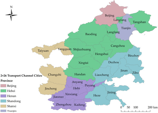
Figure 1.
“2 + 26” transport channel cities in Beijing-Tianjin-Hebei region and its surrounding areas.
Studies have been conducted on spatial correlation of air pollution from different perspectives. Some scholars focused on technological analysis, as employing air quality models for numerical simulation [10,11], which supported the cross-regional transmission of air pollution between different administrative units [12]. Qin et al. [13] simulated pollution caused by PM2.5 in the Pearl River Basin, finding cross-boundary transmission a main reason for the pollution in autumn. Scholars also adopted models based on Geographic Information System (GIS) to evaluate the geographical implications of pollutants’ dispersion [14,15]. Lee et al. [16] developed land use regression models based on GIS to evaluate outdoor NOx and NO2 concentrations in Taipei metropolis. Economists put more emphasis on the socioeconomic mechanism. Some of them adopted spatial econometrics models to verify the relationship between air pollution and economic growth [17,18]. Rupasingha et al. [19] were the first to consider spatial autocorrelation in their empirical analysis of the Environmental Kuznets Curve. Zhu et al. [20] demonstrated a significant positive spatial effect of foreign direct investment (FDI) on SO2 emission in the BTH region. Liu, Sun, and Feng [21] found the spatial agglomeration effect of environmental pollution in China with Spatial Durbin Model (SDM), and the negative spatial spillover effect in the east. Although traditional econometrics could be applied to analyze the spatial association of regional pollution, in view of the possible complex, bidirectional and multithreaded network structure of the associated pollution transport within the region, traditional methods could not illustrate complicated multithreaded spatial relations within the region, due to its general perspective as overall analysis.
Social Network Analysis (SNA) is an interdisciplinary method with “relationship” as analytical unit [22,23], with both overall analysis of a region as a whole and partial analysis for comparison of individuals within networks, which has more advantages to explain the complexity of pollution correlation network in this study. Compared with traditional econometrics, SNA has advantages in analyzing intraregional differences, for which it was chosen for this study.
SNA has already been adopted by some economists for different issues [24,25]. Cassi et al. [26] employed SNA to analyze the network and its characteristics between international trade and financial integration. Qian et al. [27] found the spatial association network of regional capital movement at provincial level in China. Some scholars started to introduce SNA to researches on environmental problems [28,29]. Liu et al. [30] discussed the spatial effect of environmental pollution in China by constructing a multithreaded network, and demonstrated the positive impact of environmental regulation and geographical proximity on the spatial spillover of environmental pollution. Several Chinese scholars evidenced spillover of air pollution by SNA, such as Liu et al. [31] and Sun et al. [32]. They analyzed the spatial association and dynamic interaction of air pollution in the Yangtze River Delta, finding the air pollution in this region a multithreaded network structure.
Researches on spatial correlation of air pollution were carried out from national [33,34], provincial [21,35] or municipal [36,37] level. Policies of air pollution control in China tend to take a city as individual, which makes it more accurate to study air pollution at municipal level. No existing literature has involved 2 + 26 policy region on regional transmission of air pollution. Besides, due to the geographical proximity and resource endowment similarity in the region, the industry sector would generate upstream and downstream industry chains or a competitive relationship, which could further lead to transmission of industrial air pollutant emissions between cities in the region [38]. Therefore, it was valuable to discuss the spatial correlation of pollutant emissions in the sampled region.
NOx is one of the nonnegligible pollutants in China. Its toxicity posed a threat to the health of residents [39,40]. Exposure to excessive NOx can result in diseases in the short term, and even death in the long term [41]. Besides, NOx can lead to the generation of PM2.5 and O3 by reacting with other elements in the atmosphere [42,43]. It also contributes to the formation of acid rain [44,45], which brings damage to the ecosystem and society. The Chinese government has realized the severity of NOx, and has defined NOx as one of the constraints of pollution emission control during the 12th Five-Year Plan (FYP). 10% and 15% emission reduction in total NOx and industrial NOx were supposed to be achieved during the 12th FYP period [46].
The trend of NOx emission in China from 2007 to 2015 is shown in Figure 2. For total NOx emission, it increased from 2007 to 2011, and declined each year from 2012 to 2015. The emission of total NOx in 2015 was 1.850 × 10¹⁰ kg, which reached the emission target of 2.046 × 10¹⁰ kg. During the sampled years, industrial NOx emission took a proportion of more than 60% in the total emission of NOx, with the similar trend curve as total NOx emission. It demonstrated that industrial sectors were the biggest contributor to the pollution of NOx. It peaked in 2011 with the emission of 1.730 × 10¹⁰ kg and decreased to 1.181 × 10¹⁰ kg in 2015. The targeted emission was 10% of the emission in 2010, i.e., 1.391 × 10¹⁰ kg, which was also achieved in 2015.
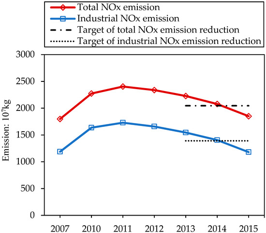
Figure 2.
Total and industrial NOx emission of China in 2007–2015.
In this study, city level data was used based on 2 + 26 policy which was issued in one of the most polluted areas in China. Since industrial NOx emission significantly contributed to NOx pollution, this research constructed a correlation network of industrial NOx emission in cities within 2 + 26 policy region based on socioeconomic elements. Due to data limitations of industrial NOx emission in the city level of China, we collected data from 2011 to 2015 through public yearbooks and local government interviews. Instead of taking traditional econometric methods, Social Network Analysis was adopted in this research, to explore the internal structure and characteristics of spatial correlation of industrial NOx emission. Different roles of 2 + 26 cities in the transmission network of industrial NOx emission are identified, in order to further define the priority of each city in the reduction strategy of industrial NOx emission. Moreover, a nonparametric method was adopted in Social Network Analysis, known as Quadratic Assignment Procedure (QAP), which provides a solution to the endogenous problem of relational data, to discuss the key influencing factors of the constructed spatial correlation network.
2. Methods and Data
2.1. Modified Gravity Model
Reilly Law was proposed in the 1930s, which extended the law of universal gravitation to social sciences [47], known as Gravity Model. This study introduces the Gravity Model based on its original definition and modification by previous literatures [29,30]. The modified Gravity Model is as follows:
where Tij is the gravity of city i to city j in transmission of industrial NOx emission, Kij is the contribution of city i to city j in transmission of industrial NOx emission. Ei and Ej stand for the air pollution in city i and city j respectively. Emission of industrial NOx is taken as a variable. Gi and Gj denote economic development of city i and city j respectively. Annual GDP of each city is adopted as an indicator. Pi and Pj represents population of city i and city j respectively, indicated by permanent resident population at the end of the year. Dij is the spatial distance between city i and city j, calculated by spherical distance between cities.
The gravity matrix of regional industrial NOx emission is constructed as binary matrix:
where I denotes the binary gravity matrix. It is measured according to Equation (4):
where Iij is the element of the binary gravity matrix, is the average value of matrix row. Elements higher than in the row were marked as 1, indicating significant spatial correlation of industrial NOx emission; elements lower than the value were marked as 0, implying insignificant spatial correlation.
2.2. Social Network Analysis
In spatial correlation network of air pollution in 2 + 26 policy region, it is possible to have complex structural features of multithread and bi-direction, in which SNA serves as a feasible tool revealing the characteristics of the complicated network.
2.2.1. Overall Indicators
Network density reflects the intensity of connection in the network. Higher density provides better economic and social conditions for cities in the region, but can also result in excessive resource dependence, which would limit the development of individual cities. Network density can be denoted as follows:
where N is the number of cities in the network, is the maximum possible connections in the network, and L represents the actual connection in the network. Dn ranges from 0 to 1.
Robustness of network can be measured by relevance [48]. Reachability is one of the indicators to test relevance in networks, which is as follows:
where C denotes reachability ranging from 0 to 1, V represents actual number of unreachable pairs in the network, and is the maximum number of unreachable pairs in the network. Higher reachability infers a more robust network.
Network efficiency is another indicator reflecting relevance of network. In the spatial correlation network of regional pollution, lower network efficiency means more pathways of pollution transport. The existence of more multiple overlying pollution associations implies worse pollution. Network efficiency can be calculated as followed:
where E represents network efficiency, ranging from 0 to 1. M is the actual number of redundant lines in the network, and max(M) is the maximum number of redundant lines in the network.
2.2.2. Centrality Analysis
To explore the position and role of cities within 2 + 26 policy region, degree centrality is employed in this research. Cites with higher degree centrality are more in the centrality of the network, which means more influential to other individuals within the region. Degree centrality can be either absolute or relative. Absolute degree centrality is the number of cities directly associated with a certain city in the network. Relative degree centrality is calculated as:
where De denotes degree centrality, n is the absolute degree centrality, and N-1 is the maximum number of cities directly associated with a certain city in the network. Relative degree centrality is adopted to ensure the comparability of the industrial NOx correlation network in different years.
Degree centrality is divided into indegree and outdegree, in order to depict the directional relationship between individuals in the network. Since the modified Gravity Model constructed a directed network, both indegree and outdegree are calculated to distinguish the direction of pollution transmission. Outdegree illustrates the pollution transmission to other cities, while indegree demonstrates the pollution transmission from other cities.
2.2.3. Quadratic Assignment Procedure
Multicollinearity may result from relational data adopted in this research. Therefore, traditional econometrics is not applicable in this research. This research adopts Quadratic Assignment Procedure to analyze influencing factors of the correlation network of industrial emission [49], as well as the geographical effect. QAP is a nonparametric test, which can avoid the problem of multicollinearity. QAP figures out the correlation coefficient between matrices by matrix permutation, which compares the similarity between elements in two matrices.
Environmental regulation and geographical effect were mainly involved as influencing factors of air pollution correlation networks, according to existing literatures [29,30]. According to the pollution haven hypothesis, enterprises tend to avoid themselves from strict environmental regulations, which leads to movement to cites with lenient environmental regulation. Environmental regulation difference, thus, might lead to the spatial transport and correlation of industrial NOx emission. Besides, neighboring cities often share frequent environmental and economic links, which makes geographical distance a possible impacting element in the correlation network of industrial NOx emission.
On such a basis, this study built the following model:
where I is the binary gravity matrix, X1 is the environmental regulation difference, and X2 stands for the geographical effect among cities.
I = f(X1, X2)
Energy intensity difference matrix was taken as a variable of environmental regulation [30,50]. Geographical effect was measured by two matrices of geographical proximity and geographical distance. Geographical proximity matrix was constructed by the standard of adjacency, with adjacent cities marked 1 and nonadjacent 0. Geographical distance matrices of 0–100 km, 100–200 km, 200–300 km, and 300–400 km were constructed, respectively, by the distance between cities. If the distance between two cities fell within the distance intervals, it was marked 1, otherwise, it was marked 0.
2.3. Data Resources
Data of industrial NOx emission came from the Annual Statistic Report on Environment in China (2011–2015) and local government investigation. Annual GDP of each city and permanent resident population at the end of the year of each city were from the China City Statistical Yearbook (2012–2016). Energy intensity was from local statistics yearbooks (2012–2016). Spatial distance was expressed by spherical distance. Annual GDP of each city took the price of 2011 as base year, with nominal GDP converted into real GDP.
3. Result and Discussion
3.1. Spatial Correlation Network of Industrial NOx
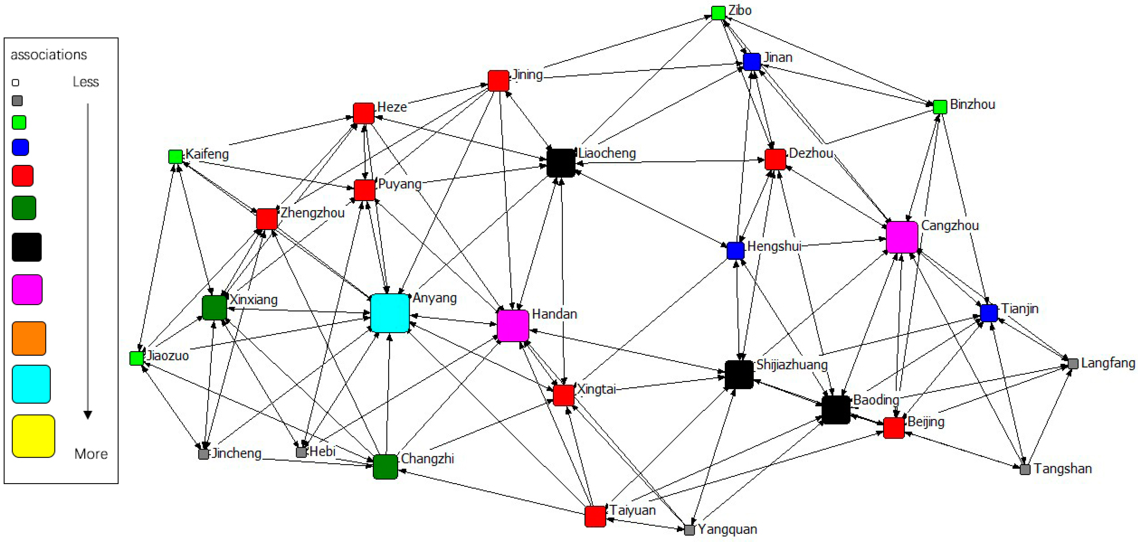
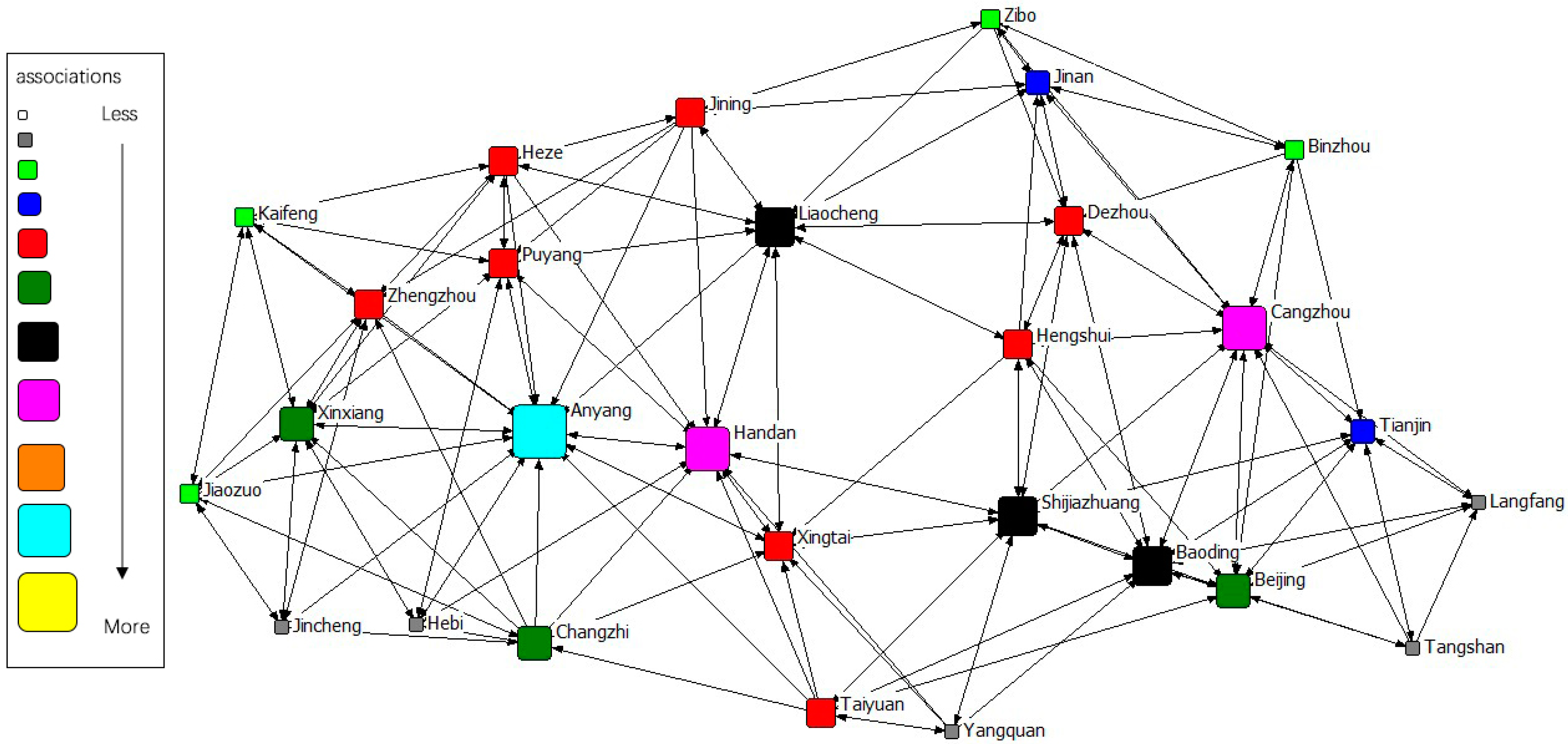
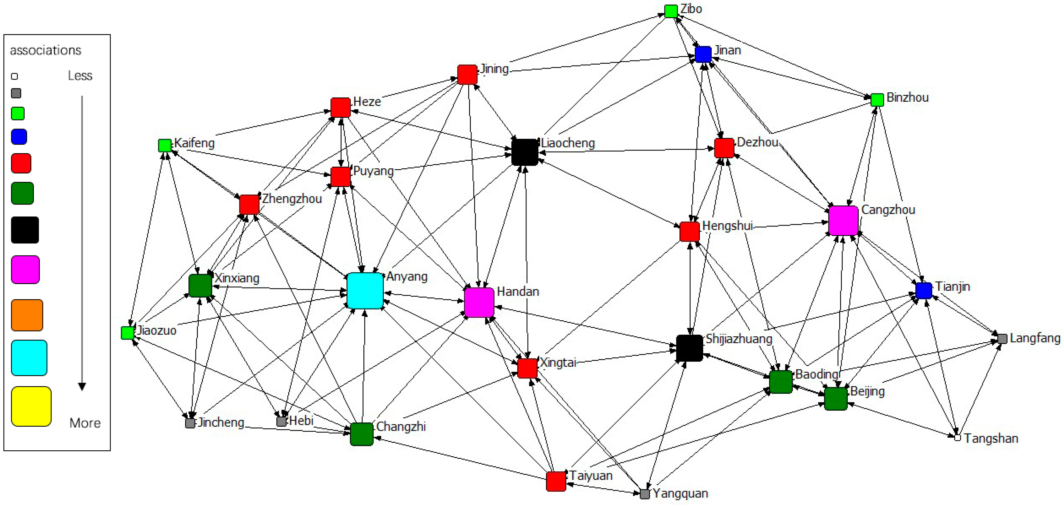
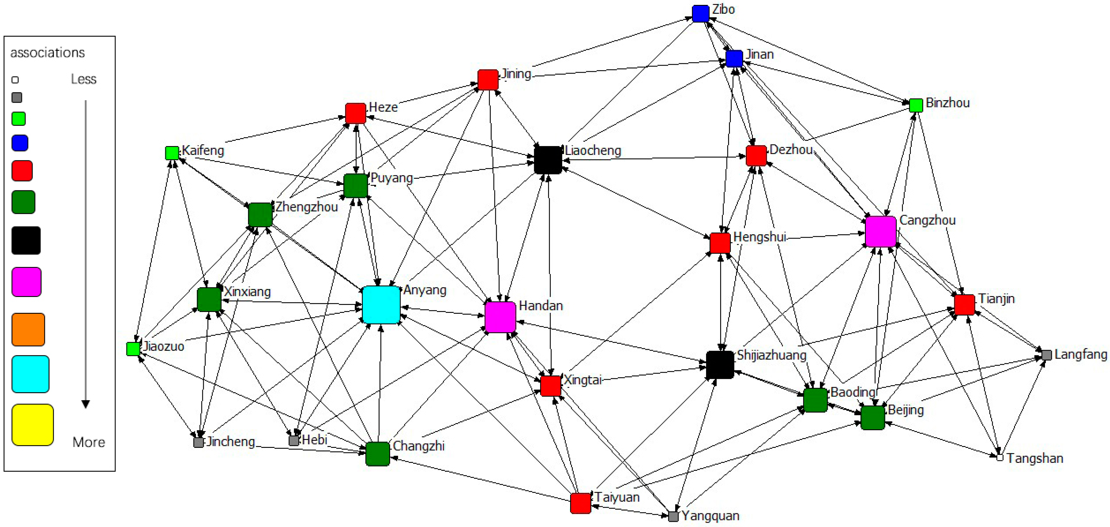
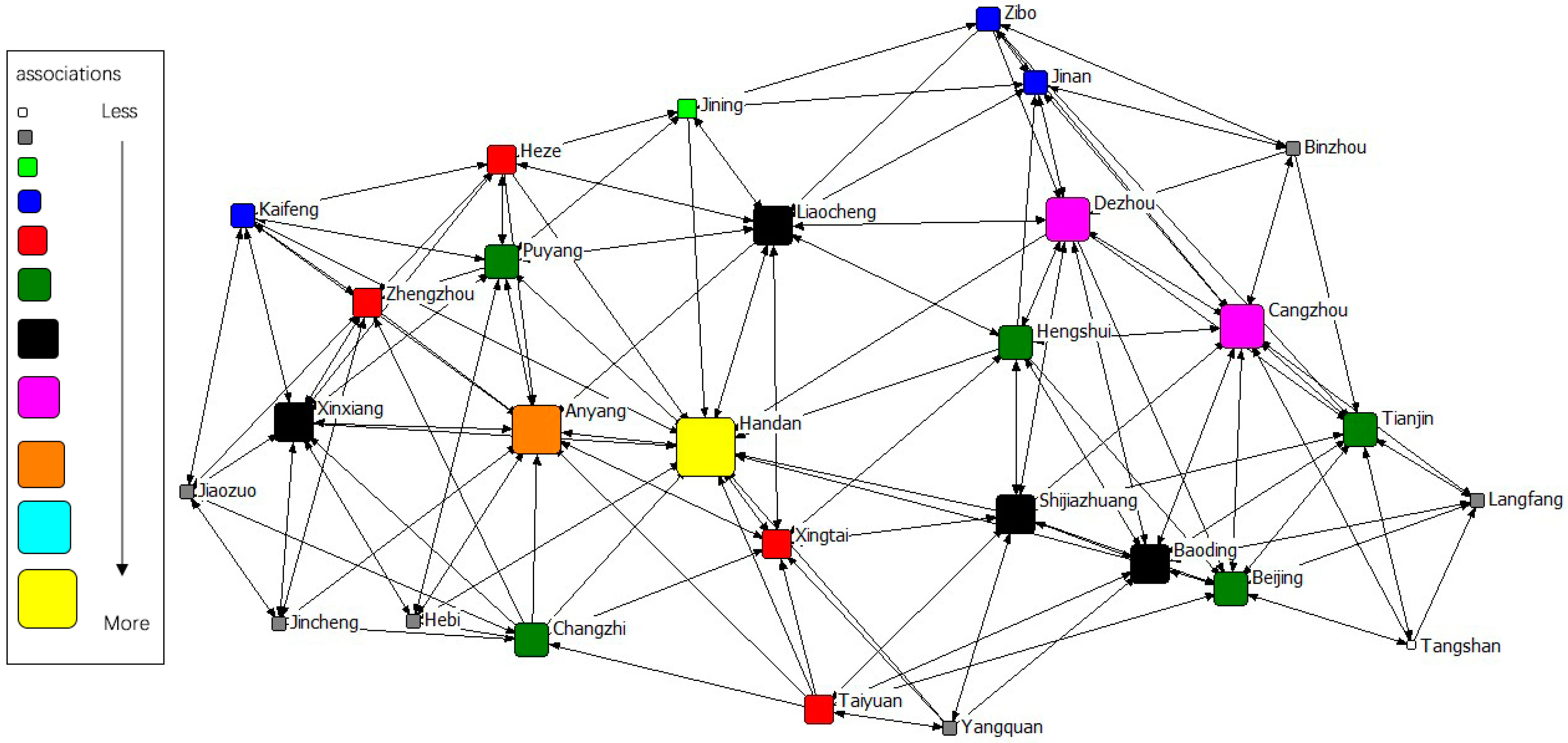
The gravity matrix of industrial NOx emission in 2 + 26 cities was calculated by the modified Gravity Model. With Ucinet 6.0, the spatial correlation network of industrial NOx emission in 2 + 26 policy region was constructed, respectively, in 2011–2015. By Netdraw, the correlation networks of industrial NOx were visualized from 2011 to 2015. Results of year 2011 to 2015 are displayed in Figure 3, Figure 4, Figure 5, Figure 6 and Figure 7. It might also be noted that, arrows and lines in Figure 3, Figure 4, Figure 5, Figure 6 and Figure 7 indicate significant pollution transmission from one city to another. No arrow or line means the pollution transmission between the two was not significant. The squares from small to large in Figure 3, Figure 4, Figure 5, Figure 6 and Figure 7 represent the number of related cities from less to more, which indicates the associations of a certain city in the network. To better compare the results in different years, different colors were used to indicate the exact quantity of related cities. Cities with the same square size share the same color.
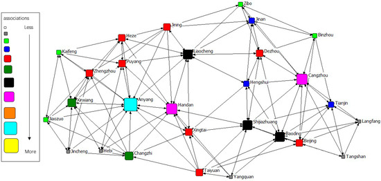
Figure 3.
Spatial correlation network of industrial NOx emission in 2 + 26 policy region, 2011.
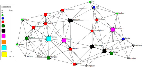
Figure 4.
Spatial correlation network of industrial NOx emission in 2 + 26 policy region, 2012.
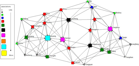
Figure 5.
Spatial correlation network of industrial NOx emission in 2 + 26 policy region, 2013.
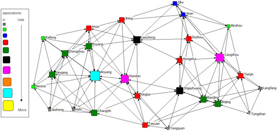
Figure 6.
Spatial correlation network of industrial NOx emission in 2 + 26 policy region, 2014.
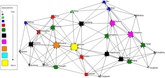
Figure 7.
Spatial correlation network of industrial NOx emission in 2 + 26 policy region, 2015.
The results indicated a relatively stable network structure of industrial NOx emission from 2011 to 2015. Intercity correlation, on the other hand, showed interannual differences. Some cities remained the same in connection with other cities during the 5 years, including Langfang, Cangzhou, Taiyuan, Yangquan, Changzhi, Jincheng, Liaocheng, Heze and Hebi. The correlation of other cities changed in different years. For example, the NOx emission of Anyang was most connected with that of other cities in 2011–2014, but was replaced by Handan in 2015. Some disconnected cities became correlated; for instance, the NOx emission in Handan and Dezhou had no significant relationship during 2011–2014, but became correlated in 2015. Some connected cities in a certain year showed no significant correlations in other years, such as Anyang and Jining in 2015. Compared with the network in 2011, the network in 2015 had the most significant difference. 16 cities had changes in their connections, including Handan, Kaifeng, Xintai, Dezhou, Hengshui, Baoding, Tianjin, Zibo, Beijing, Zhengzhou, Puyang, Shijiazhuang, Binzhou, Anyang, Jiaozuo, and Jining.
3.2. Characteristics of the Network Structure
3.2.1. Overall Characteristics
Network correlation and density of industrial NOx emission in 2 + 26 cities were measured through Ucinet 6.0. The results are shown in Figure 8. The correlation and density of spatial correlation network fluctuated slightly over five years, which meant the spatial transmission of industrial NOx emission in this region remained largely stable.
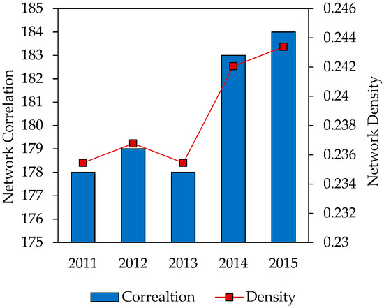
Figure 8.
Network density of industrial NOx emission in 2011–2015.
Reachability of the network of industrial NOx emission in 2011 to 2015 remained at 1, indicating significant robustness of air pollution correlation among 2 + 26 policy region. Network efficiency, as in Table 1, also showed stability with minor fluctuations, which proved the stable spatial correlation network of industrial NOx emission in the sampled region within five years.

Table 1.
Network efficiency of emission of industrial NOx in 2011–2015.
3.2.2. Individual Characteristics
The standardized relative degree centrality of 2 + 26 cities in the correlation network of industrial NOx emission are calculated by Ucinet 6.0. Outdegree and indegree in 2011–2015 are shown in Table 2. Cities with high outdegree were authorities in the network, which was more influential as the sources during the pollution transmission of industrial NOx emission. Shijiazhuang remained the highest outdegree in 2011–2015. Cities with high indegree were hubs in the network, receiving heavier pollution during the transmission of industrial NOx emission. Cities with the highest indegree were Anyang in 2011–2012, Cangzhou in 2013–2014 and Handan in 2015. Cities with low indegree or outdegree indicated marginalization of reception or delivery during pollution transmission, which indicated little impact on network. Langfang and Hebi remained the lowest of outdegree in 2011–2015, Xingtai in 2011–2012, and Jincheng in 2013–2014. Taiyuan, Yangquan and Tangshan had the lowest indegree in 2011–2015.

Table 2.
The standardized degree of industrial NOx emission network in 2011–2015.
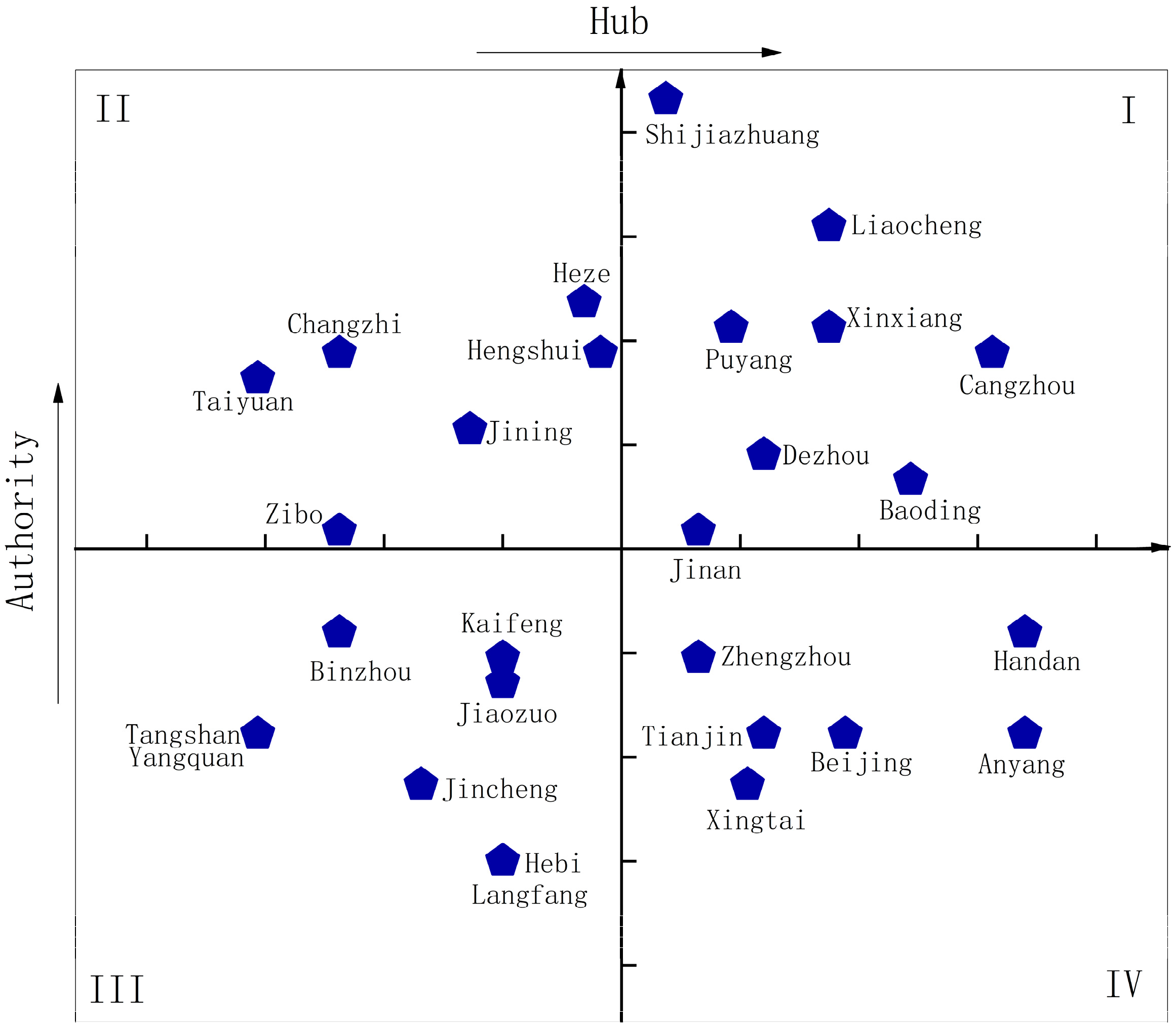
To better evaluate the city characteristics over the five years, the average outdegree and indegree of each city were calculated and after, standardized, to determine the position trend of cities in the network, as shown in a quadrant scatter chart of Figure 9. Since outdegree and indegree respectively reflect the occurrence of delivery and reception for pollutant emission from a certain city to other cities, cities were further distinguished as authority or hub according to the average outdegree and indegree after standardization. Four quadrants in the scatter chart, marked I, II, III and IV, divided cities in the region into four types: high-high, high-low, low-low, and low-high, indicating positions of a city as high authority and hub, high authority but low hub, low authority, and hub and low authority but high hub in the network.
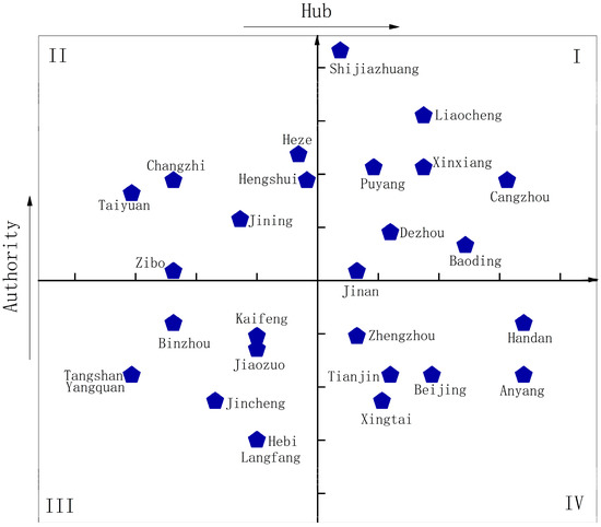
Figure 9.
The position trend of each city in the industrial NOx emission network.
Due to different characteristics of cities, differentiated strategies should be implemented for pollutant reduction and control. Cities of the high-high type were both strong authorities and hubs; therefore, they should be taken as key targets in reduction of regional industrial NOx emission. Both local emission reduction and intercity cooperation should be stressed for better reduction effect, with special attention given to competitive, or upstream and downstream enterprises in other cities, to alleviate the problem of transregional air pollution. Cities of the high-low type could easily impact other cities with their industrial NOx emissions, but were less likely to be influenced in return. The emission reduction strategy of this type should focus on the local emission, which was beneficial for other cities and themselves. As for the low-low type, such cities were neither authorities nor hubs compared to other cities. However, it was the position trend of a city in the network, not the city itself, being discussed in this research. Thus, the emission effect of a city on itself should also be measured, combined with its emission situation. Cities of this type should determine their emission-reducing strategies based on their own emissions. Cities with a relatively high level of industrial NOx emission should first improve the local pollution, to satisfy the basic emission standard. Cities up to basic standard of industrial NOx emission should be encouraged to employ a less strict strategy for saving costs. For low-high type cities which mostly acted as hubs, they were vulnerable authorities, and more susceptible to emissions from other cities. Their emission reduction strategies should emphasize intercity emission reduction, especially focusing on competitive, upstream or downstream enterprises concerning other cities.
Moreover, based on previous literatures [51], the core cities and the edge cities were determined by degree centrality (indegree or outdegree) of all years ranking top (bottom) 5, as in Table 2. The results showed that, Shijiazhuang, Liaocheng, Heze, and Xinxiang always ranked among the top few in outdegree from 2011–2015, indicating larger contribution to pollution delivery in the network; Cangzhou and Handan featured top-ranking indegrees to more pollution reception in the network. Shijiazhuang, Liaocheng, Xinxiang and Cangzhou were high-high cities to be given special attention in reduction of industrial NOx emission. Heze was a high-low type city that should emphasize local emission reduction. Handan, a low-high type city, needed to focus on intercity emission reduction, in order to prevent it from being excessively impacted by emissions from other cities.
Hebi and Langfang always ranked among the last few in outdegree over 2011–2015, as they showed a small contribution to the output emissions in the network; Tangshan, Taiyuan and Yangquan always ranked bottom in indegree, evidencing little reception of emissions in the network. Combined with city types, the reduction emission strategies can be worked out. As a city of high-low type, Taiyuan, though it received fewer emissions from the outside, should focus on local industrial pollution to prevent the impact on its surrounding cities. Hebi, Langfang, Tangshan and Yangquan, as low-low type cities, were marginalized in both outdegree and indegree, meaning that improvement in their emission result gave little contribution to the overall air pollution of the network. However, these cities should still guarantee their local industrial emissions up-to-standard, avoiding local environmental effects of industrial NOx emission.
4. Influencing Factors of the Correlation Network of Industrial NOx Emission
QAP regression of the industrial NOx emission correlation network by year is shown in Table 3. Measurement of geographical effect was done by the matrix of geographical proximity (Column 1) and the matrix of geographical distance (Column 2). The impact of environmental regulation and geographical effect are both discussed in the following.

Table 3.
QAP Regression Results of Industrial NOx Emission.
Results in Table 3 demonstrated negative coefficients of environmental regulation difference in the spatial correlation network of industrial NOx emission, with insignificance from 2011 to 2013, and significance at 1% level in 2014–2015, which showed the narrowed difference in environmental regulation would lead to a more intensive correlation network. Column 1 and Column 2 showed consistency in regression coefficient and significance level of environmental regulation difference, implying robustness of the regression. A bounce-back in industrial NOx emission might be a feasible explanation due to the continued national policy for energy consumption reduction. To be specific, in response to the national policy on energy saving and emission reduction, enterprises in the region invested heavily in energy intensity reduction. When energy consumption was brought down to a certain level, and energy efficiency up to a higher level, the difference among cities in energy intensity would be narrowed naturally. Nevertheless, as energy consumption continued to decrease, the marginal cost for lower energy consumption would increase, whereas enterprises might substantially increase their output for cost recovery, thus worsening pollution and spatial spillover of industrial NOx emission. The bounce-back effect of industrial NOx emission had no significant effect on the spatial correlation network before 2014. Since 2014, with the environmental regulation difference becoming significant at 1% level, the bounce-back has produced significant negative impact.
According to Column 1 in Table 3, of the regression by the geographical proximity matrix, the adjusted R2 was acceptable in each year with fluctuations in 28.8%–31.2%. The geographical proximity matrix rejected the original hypothesis at the significant level of 1% in each year of 2011–2015, with positive coefficients, verifying a positive relationship between industrial NOx emission and geographical proximity in 2 + 26 policy region. Reliable explanations were obtained in Column 2, with the adjusted R2 from 56.5% to 58.2% in each year. Geographical distance matrices of 0–100 km and 100-200 km remained significantly positive at 1% level; the matrix of 200–300 km passed the test of significance at 5% level, showing positive effect; and the matrix of 300–400 km failed the test of significance. The emission of industrial NOx had significant spatial correlation in cities within the distance of 0–300 km, while no significant spatial correlation when exceeding 300 km.
Results demonstrated positive geographical effect on the spatial correlation network of industrial NOx emission. Moreover, the significance level of the geographical distance matrix reduced as the geographic distance increased, meaning that the spatial correlation of industrial NOx emission weakened gradually with the widening distance. Regression coefficients of the geographical distance matrix strengthened such findings. Figure 10 illustrated the trend of regression coefficients of the geographical distance matrix in the spatial correlation network over 2011–2015. Coefficients of the same geographical distance matrix remained stable in 2011–2015, but evidenced a cascade decrease of matrices with different distances. Closer geographical distance influenced spatial correlation of industrial NOx emission more severely, which further supported the existence of geographical distance effect.
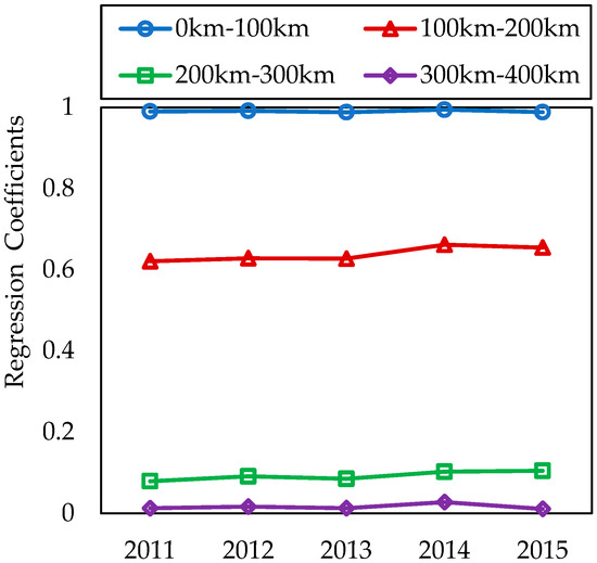
Figure 10.
The coefficient trend of geographical distance effect in industrial NOx emission network.
5. Conclusions
The spatial correlation network of industrial NOx emission was constructed based on a modified Gravity Model and Social Network Analysis. It revealed a stable structure in the network according to network density, reachability and efficiency. Correlation of industrial NOx emission received less impact from the background of emission decline of industrial NOx and economic upswing.
Cities in 2 + 26 policy region were categorized into 4 types by the position of cities in the spatial correlation network of industrial NOx emission: high-high type, high-low type, low-low type and low-high type. Shijiazhuang, Puyang, Liaocheng, Dezhou, Xinxiang, Cangzhou, Jinan, Baoding and Hengshui are high-high type cities. Taiyuan, Changzhi, Zibo, Jining and Heze belong to high-low type. Low-low type includes Kaifeng, Jiaozuo, Langfang, Hebi, Jincheng, Bingzhou, Yangquan and Tangshan. Low-high type consists of Zhengzhou, Xingtai, Tianjin, Beijing, Anyang and Handan. Appropriate emission reduction strategies ought to be implemented corresponding to characteristics of each city type. Cities of the high-high type should stress both local emission reduction and intercity collaboration; the high-low type should focus mainly on local emission so as to avoid exporting pollution to other cities; the low-low type may adopt rather relaxed emission reduction policy on the premise that their own emission levels are up-to-standard; and the low-high type should pay more attention to intercity emission reduction.
Core cities in the network are Shijiazhuang, Liaocheng, Cangzhou, Heze, and Handan. Shijiazhuang, Liaocheng, and Cangzhou should be listed as key monitoring cities in industrial NOx emission reduction. Heze should be a key city for local emission reduction, and Handan, a special focus of intercity emission reduction. Edge cities include Hebi, Langfang, Tangshan, Taiyuan, and Yangquan. Despite its marginalization of pollution reception in the network, Taiyuan still contributed to pollution delivery. It should prioritize the local industrial emissions reduction to avoid air pollution spillover to its neighboring cities. Hebi, Langfang, Tangshan and Yangquan share little links with other cities, but should first standardize local industrial emissions based on their current industrial NOx emission.
Influencing factors of the spatial transport network of industrial NOx emission involve environmental regulation difference and geographical effect. Environmental regulation difference has projected a significant negative effect on the spatial correlation network of industrial NOx emission since 2014; the possible reason behind this being the bounce-back of industrial NOx emission caused by increased output of enterprises trying to seek more profit under the national policy of energy consumption reduction. The geographical proximity matrix and the geographical distance matrix both have a significant positive effect on the spatial correlation network of industrial NOx emission. Meanwhile, spatial correlation of industrial NOx emission features a significant geographical distance effect, with the significance of the geographical distance matrix lowering as the distance stretches longer; i.e., the spatial transport of industrial NOx emission weakens gradually as geographical distance increases. Specifically, industrial NOx emission of cities within the distance range of 0–300 km is of significant spatial correlation; exceeding the spatial distance of 300 km, the spatial transport will no longer be significant.
Author Contributions
Conceptualization, X.T., L.S., Z.M. and G.L.; methodology, S.J.; software, S.J. and Y.W.; validation, X.T.; formal analysis, S.J. and Y.W.; investigation, X.X.; resources, S.J., Y.W. and L.S.; writing—original draft preparation, S.J.; writing—review and editing, S.J., X.T., L.S., R.C., Z.M. and G.L.; visualization, S.J.; supervision, X.T., L.S., R.C., Z.M. and G.L.; project administration, L.S. and Z.M.; funding acquisition, S.J. and L.S. All authors have read and agreed to the published version of the manuscript.
Funding
This research was funded by National Key R&D Program of China (2018YFC0213702), and supported by the Outstanding Innovative Talents Cultivation Funded Programs 2019 of Renmin University of China.
Conflicts of Interest
The authors declare no conflict of interest.
References
- Anselin, L. Spatial Effects in Econometric Practice in Environmental and Resource Economics. Am. J. Agr. Econ. 2001, 83, 705–710. [Google Scholar] [CrossRef]
- Pinault, L.; Crouse, D.; Jerrett, M.; Brauer, M.; Tjepkema, M. Spatial associations between socioeconomic groups and NO2 air pollution exposure within three large Canadian cities. Environ. Res. 2016, 147, 373–382. [Google Scholar] [CrossRef] [PubMed]
- Wang, W.-Q.; Ying, Y.-Y.; Wu, Q.-Y.; Zhang, H.-P.; Ma, D.-D.; Xiao, W. A GIS-based spatial correlation analysis for ambient air pollution and AECOPD hospitalizations in Jinan, China. Respir. Med. 2015, 109, 372–378. [Google Scholar] [CrossRef] [PubMed]
- Maddison, D. Modelling sulphur emissions in Europe: A spatial econometric approach. Oxf. Econ. Pap. 2007, 59, 726–743. [Google Scholar] [CrossRef]
- Sun, C.-Z.; Yang, Y.-D.; Zhao, L.-S. Economic spillover effects in the Bohai Rim Region of China: Is the economic growth of coastal counties beneficial for the whole area? China Econ. Rev. 2015, 33, 123–136. [Google Scholar] [CrossRef]
- Song, C.-B.; Lin, W.; Xie, Y.-C.; He, J.-J.; Xi, C.; Wang, T.; Lin, Y.-C.; Jin, T.-S.; Wang, A.-X.; Yan, L. Air pollution in China: Status and spatiotemporal variations. Environ. Pollut. 2017, 227, 334–347. [Google Scholar] [CrossRef]
- Liu, H.; Tian, Y.-H.; Xu, Y.; Huang, Z.; Huang, C.; Hu, Y.-H.; Zhang, J. Association between ambient air pollution and hospitalization for ischemic and hemorrhagic stroke in China: A multicity case-crossover study. Environ. Pollut. 2017, 230, 234–241. [Google Scholar] [CrossRef]
- Lelieveld, J.; Evans, J.; Fnais, M.; Giannadaki, D.; Pozzer, A. The contribution of outdoor air pollution sources to premature mortality on a global scale. Nature 2015, 525, 367–371. [Google Scholar] [CrossRef]
- Notice on Printing Detailed Implementing Plan for Air Pollution Control in the Beijing-Tianjin-Hebei Region and Surrounding Areas. Available online: http://www.mee.gov.cn/gkml/hbb/bwj/201309/t20130918_260414.htm (accessed on 17 February 2020).
- Fan, Q.; Yu, W.; Fan, S.-J.; Wang, X.-M.; Lan, J.; Zou, D.-L.; Feng, Y.-R.; Chan, P.W. Process analysis of a regional air pollution episode over Pearl River Delta Region, China, using the MM5-CMAQ model. J. Air Waste Manag. Assoc. 2014, 64, 406–418. [Google Scholar] [CrossRef]
- Wang, H.; Xue, M.; Zhang, X.-Y.; Liu, H.; Zhou, C.-H.; Tan, S.; Che, H.-Z.; Chen, B.; Li, T. Mesoscale modeling study of the interactions between aerosols and PBL meteorology during a haze episode in Jing–Jin–Ji (China) and its nearby surrounding region—Part 1: Aerosol distributions and meteorological features. Atmos. Chem. Phys. 2015, 15, 3257–3275. [Google Scholar] [CrossRef]
- Hu, J.-L.; Wang, Y.-G.; Ying, Q.; Zhang, H.-L. Spatial and temporal variability of PM2.5 and PM10 over the North China Plain and the Yangtze River Delta, China. Atmos. Environ. 2014, 95, 598–609. [Google Scholar] [CrossRef]
- Qin, M.-M.; Wang, X.-S.; Hu, Y.-T.; Huang, X.-F.; He, L.-Y.; Zhong, L.-J.; Song, Y.; Hu, M.; Zhang, Y.-H. Formation of particulate sulfate and nitrate over the Pearl River Delta in the fall: Diagnostic analysis using the Community Multiscale Air Quality model. Atmos. Environ. 2015, 112, 81–89. [Google Scholar] [CrossRef]
- Briggs, D. The Role of Gis: Coping With Space (And Time) in Air Pollution Exposure Assessment. J. Toxicol. Environ. Health Part A 2005, 68, 1243–1261. [Google Scholar] [CrossRef] [PubMed]
- Famoso, F.; Wilson, J.; Monforte, P.; Lanzafame, R.; Brusca, S.; Lulla, V. Measurement and modeling of ground-level ozone concentration in Catania, Italy using biophysical remote sensing and GIS. Int. J. Appl. Eng. Res. 2017, 12, 10551–10562. [Google Scholar]
- Lee, J.-H.; Wu, C.-F.; Hoek, G.; de Hoogh, K.; Beelen, R.; Brunekreef, B.; Chan, C.-C. Land use regression models for estimating individual NOx and NO2 exposures in a metropolis with a high density of traffic roads and population. Sci. Total Environ. 2014, 472, 1163–1171. [Google Scholar] [CrossRef]
- Zeng, J.-Y.; He, Q.-Q. Does industrial air pollution drive health care expenditures? Spatial evidence from China. J. Clean. Prod. 2019, 218, 400–408. [Google Scholar] [CrossRef]
- Li, M.; Li, C.; Zhang, M. Exploring the spatial spillover effects of industrialization and urbanization factors on pollutants emissions in China’s Huang-Huai-Hai region. J. Clean. Prod. 2018, 195, 154–162. [Google Scholar] [CrossRef]
- Rupasingha, A.; Goetz, S.; Debertin, D.; Pagoulatos, A. The environmental Kuznets curve for US counties: A spatial econometric analysis with extensions. Pap. Reg. Sci. 2004, 83, 407–424. [Google Scholar] [CrossRef]
- Zhu, L.; Gan, Q.-M.; Liu, Y.; Yan, Z.-J. The impact of foreign direct investment on SO2 emissions in the Beijing-Tianjin-Hebei region: A spatial econometric analysis. J. Clean. Prod. 2017, 166, 189–196. [Google Scholar] [CrossRef]
- Liu, X.-R.; Sun, T.; Feng, Q. Dynamic spatial spillover effect of urbanization on environmental pollution in China considering the inertia characteristics of environmental pollution. Sustain. Cities Soc. 2020, 53, 101903. [Google Scholar] [CrossRef]
- Oliveira, M.; Gama, J. An overview of social network analysis. WIREs Data Min. Knowl. Discov. 2012, 2, 99–115. [Google Scholar] [CrossRef]
- Yokura, Y.; Matsubara, H.; Sternberg, R. R&D networks and regional innovation: A social network analysis of joint research projects in Japan. Area 2013, 45, 493–503. [Google Scholar] [CrossRef]
- Snyder, D.; Kick, E. Structural Position in the World System and Economic Growth, 1955–1970: A Multiple-Network Analysis of Transnational Interactions. Am. J. Sociol. 1979, 84, 1096–1126. [Google Scholar] [CrossRef]
- Chase-Dunn, C.; Grimes, P. World-Systems Analysis. Annu. Rev. Sociol. 2003, 21, 387–417. [Google Scholar] [CrossRef]
- Cassi, L.; Morrison, A.; Ter Wal, A. The Evolution of Trade and Scientific Collaboration Networks in the Global Wine Sector: A Longitudinal Study Using Network Analysis. Econ. Geogr. 2012, 88, 311–334. [Google Scholar] [CrossRef]
- Qian, X.-H.; Wang, Y.; Zhang, G.-L. The spatial correlation network of capital flows in China: Evidence from China’s High-Value Payment System. China Econ. Rev. 2018, 50, 175–186. [Google Scholar] [CrossRef]
- Salpeteur, M.; Calvet-Mir, L.; Díaz-Reviriego, I.; Reyes-García, V. Networking the environment: Social network analysis in environmental management and local ecological knowledge studies. Ecol. Soc. 2017, 22, 41. [Google Scholar] [CrossRef]
- Chen, Y.-T.; Ge, C.-Z.; Duan, X.-M. Researches on SO2 Emission Network Structure and Its Determinants in the Yangtze River Economic Belt. Ecol. Econ. 2017, 33, 143–148. [Google Scholar]
- Liu, H.-J.; Liu, C.-M.; Yang, Q. Spatial spillover and the source of environment pollution—Empirical study on the perspective of network analysis. Economist 2015, 10, 28–35. [Google Scholar] [CrossRef]
- Liu, H.-J.; Liu, C.-M. Air pollution’s nonlinear transmission among cities and its co-movement network in Jing-Jin-Ji Region. Chin. J. Popul. Sci. 2016, 84–95. [Google Scholar]
- Sun, Y.-N.; Xiao, C.-X.; Liu, H.-J. Air pollution’s urban linkage and dynamic interaction in Yangtze River Delta Region—Based on AQI data empirical study. Rev. Econ. Manag. 2017, 121–131. [Google Scholar] [CrossRef]
- Balado-Naves, R.; Baños-Pino, J.F.; Mayor, M. Do countries influence neighbouring pollution? A spatial analysis of the EKC for CO2 emissions. Energy Policy 2018, 123, 266–279. [Google Scholar] [CrossRef]
- Antonakakis, N.; Chatziantoniou, I.; Filis, G. Energy consumption, CO2 emissions, and economic growth: An ethical dilemma. Renew. Sustain. Energ. Rev. 2017, 68, 808–824. [Google Scholar] [CrossRef]
- Chen, S.-M.; Zhang, Y.; Zhang, Y.-B.; Liu, Z.-X. The relationship between industrial restructuring and China’s regional haze pollution: A spatial spillover perspective. J. Clean. Prod. 2019, 239, 11508. [Google Scholar] [CrossRef]
- Du, Y.-Y.; Sun, T.-S.; Peng, J.; Fang, K.; Liu, Y.-X.; Yang, Y.; Wang, Y.-L. Direct and spillover effects of urbanization on PM2.5 concentrations in China’s top three urban agglomerations. J. Clean. Prod. 2018, 190, 72–83. [Google Scholar] [CrossRef]
- Xu, X.-X.; Wang, Y.-H. Study on Spatial Spillover Effects of Logistics Industry Development for Economic Growth in the Yangtze River Delta City Cluster Based on Spatial Durbin Model. Int. J. Environ. Res. Public Health 2017, 14, 1508. [Google Scholar] [CrossRef]
- Liu, H.-J.; Liu, C.-M.; Chen, M. The Conduction Network and Collaborative Reduction among Different Industries of Carbon Dioxide Emission in China’s Industries. China Popul. Resour. Environ. 2016, 26, 90–99. [Google Scholar] [CrossRef]
- Kurvits, T.; Marta, T. Agricultural NH3 and NOx emissions in Canada. Environ. Pollut. 1998, 102, 187–194. [Google Scholar] [CrossRef]
- Wei, C.-C.; Lin, H.-J.; Lim, Y.-P.; Chen, C.-S.; Chang, C.-Y.; Lin, C.-J.; Chen, J.J.-Y.; Tien, P.-T.; Lin, C.-L.; Wan, L. PM2.5 and NOx exposure promote myopia: Clinical evidence and experimental proof. Environ. Pollut. 2019, 254, 113031. [Google Scholar] [CrossRef]
- Diao, B.-D.; Ding, L.; Su, P.-D.; Cheng, J.-H. The Spatial-Temporal Characteristics and Influential Factors of NOx Emissions in China: A Spatial Econometric Analysis. Int. J. Environ. Res. Public Health 2018, 15, 1405. [Google Scholar] [CrossRef]
- Wang, N.; Lyu, X.-P.; Deng, X.-J.; Huang, X.; Jiang, F.; Ding, A.-J. Aggravating O3 pollution due to NOx emission control in eastern China. Sci. Total Environ. 2019, 677, 732–744. [Google Scholar] [CrossRef] [PubMed]
- Song, W.; Wang, Y.-L.; Yang, W.; Sun, X.-C.; Tong, Y.-D.; Wang, X.-M.; Liu, C.-Q.; Bai, Z.-P.; Liu, X.-Y. Isotopic evaluation on relative contributions of major NOx sources to nitrate of PM2.5 in Beijing. Environ. Pollut. 2019, 248, 183–190. [Google Scholar] [CrossRef] [PubMed]
- Boningari, T.; Smirniotis, P.G. Impact of nitrogen oxides on the environment and human health: Mn-based materials for the NOx abatement. Curr. Opin. Chem. Eng. 2016, 13, 133–141. [Google Scholar] [CrossRef]
- Gómez-García, M.A.; Pitchon, V.; Kiennemann, A. Pollution by nitrogen oxides: An approach to NOx abatement by using sorbing catalytic materials. Environ. Int. 2005, 31, 445–467. [Google Scholar] [CrossRef]
- Notice of the State Council on Issuing the Plan for Energy Conservation and Emission Reduction during the “Twelfth Five-Year Plan” Period (No. 40 [2011]). Available online: http://www.gov.cn/zhengce/content/2012-08/12/content_2728.htm (accessed on 17 February 2020).
- Reilly, W.J. The law of Retail Gravitation; Knickerbocker Press: Albany, NY, USA, 1931; p. 183. [Google Scholar]
- Krackhardt, D. Graph Theoretical Dimensions of Informal Organization. Comput. Organ. Theory 1994, 89–111. [Google Scholar] [CrossRef]
- Liu, J. Lectures on Whole Network Approach: A practical guide to UCINET, 2nd ed.; Truth & Wisdom Press: Shanghai, China, 2014; p. 357. [Google Scholar]
- Jiang, K.; Lu, X.-X. Research on the measurement of environmental regulation variables. Stat. Decis. 2011, 19–22. [Google Scholar] [CrossRef]
- Zhang, D.-G.; Lu, Y.-Q. Study on the Spatial Correlation and Explanation of Carbon Emission in China—Based on Social Network Analysis. Soft Sci. 2017, 31, 15–18. [Google Scholar]
© 2020 by the authors. Licensee MDPI, Basel, Switzerland. This article is an open access article distributed under the terms and conditions of the Creative Commons Attribution (CC BY) license (http://creativecommons.org/licenses/by/4.0/).


