Article

An Optimization Management Model for Countries with Mutually Competitive Regions

1
School of Mathematics and Statistics, North China University of Water Resources and Electric Power, Zhengzhou 450045, China
2
School of Economics and Finance, Xi’an Jiaotong University, Xi’an 710061, China
3
Shaanxi Institute of Socialism, Xi’an 710061, China
*
Author to whom correspondence should be addressed.
Sustainability 2020, 12(6), 2326; https://doi.org/10.3390/su12062326
Submission received: 11 February 2020 / Revised: 7 March 2020 / Accepted: 10 March 2020 / Published: 17 March 2020

Abstract

:
It is difficult to manage resources allocation and pollution in a multi-regional country with mutually competitive relations. This work therefore intends to propose an optimal control model for the management problem. Through introducing the union utility function to model competitive interactions, we construct an integrated economy, resource, and environment macroeconomic model according to the social practices in the country with some competitive regions. Numerical procedures are proposed to search for the optimal energy policy and antipollution strategy of the model. As shown, an optimal fair tradeoff between efficiency and equity can be balanced for each region in the country. More important, the model verifies the importance of the role of government for management problems in a country with complex internal competitive relations

1. Introduction

For an economic system with competitive individuals, each individual will only pursue the maximization of their own profits, if there is no powerful management from the government. It usually leads to the Nash equilibrium according to the non-cooperative game theory [1]. However, the Nash equilibrium is suboptimal to the system. It is necessary to introduce one government to bring more profits for the whole system. The presence of government makes the optimal solution of the system more like a cooperative game equilibrium [2], where the role of the government is to ensure more profits for the economic system.
These systems with internal competitive relations widely exist in various scientific and social applications. Here, the “competitive” means that each region competes for the scare resource and they all try to obtain as more as possible to meet their own urgent needs. In this work, we consider energy resource development to illustrate the management problem in a multi-competitive-region country. We intend to accurately model the systems with internal competitiveness from the perspective of optimization. Since energy resource use worsens the environmental quality when improving the life quality of human beings, it is necessary for us to develop energy resources while controlling the pollution for a sustainable energy resource development. In the model, it is also necessary to characterize the internal relations, which is of vital importance for the harmonic development of a country with many regions.
Generally, two theoretical frameworks are applicable to the management problem: one is based on the Integrated Assessment Models (IAMs); the other is related to optimum control theory.
The IAMs are suggested to comprehensively evaluate greenhouse gas emissions by integrating scientific theories and technical methods of natural and social science. The global warming model was firstly suggested by Nordhaus in 1991 [3]. Then on this base, the DICE (the Dynamic Integrated Model of Climate and the Economy) was developed in 1994 and is of broad influence [4]. Presently, there are approximately 20 actively used models in development and use. In China, the most representative is the I\O-INET model developed by the scholars from Tsinghua University [5]. In general, the computation scale of the IAMs is usually very large and computer simulation is needed.
Roughly speaking, optimization management is to determine the optimal control paths of control variables in a dynamic optimization system. The Forster models are proposed to determine the optimal energy use for energy development in [6,7]. Zhong and Li (2002) suggest a dynamic optimization model on global warming, and analyze the emission reduction policy as well as its economy-environment affects [8]. Zhu and Wang etc. demonstrate that the productivity of energy resources is critical to improve the environmental quality [9]. For further studies on climate policy using dynamic optimizing models, one may refer to [10].
However, these models are still far from realities, since they only consider the emissions of greenhouse gas in one single region without involving the internal relationship between different regions. Hence, multi-regional modelling has attracted more attention and interest in the area of optimization management. Leimbach and Eisenack propose the multi-regional model, which represents a dynamic model of international trade based on a trade algorithm [11]. It is shown that there exist complex and nonlinear relations between different regions, especially when the relations of these regions are competitive.
Li and Zhong have provided the two-regional control model to simulate the mutual increasing and decreasing competition of different regions in [12]. But their model is not accurate enough and practical, since it is limited only to nonlinear competitive relations of different regions and the nonlinearity is not accurately characterized. In practical problems, various relations, whether it is linear or nonlinear, may exist and be coupled with each other in different regions simultaneously. It is necessary for the management agency or the government to present an overall optimization plan according to concrete internal relations. More accurately, the real relationship in a country should be described as competition in cooperation or cooperation in competition. A fair resource allocation will provide each region with proper satisfactions, and keep the balance of the system at the same time. While, on the contrary, unfair resource allocation will lead to strong resistances from those regions that do not receive sufficient resources.
To this end, we mean to develop strategies to reasonably allocate resources in a multi-regional country in this work. We will extend the concept of union utility function to construct a more accurate optimization model with mutually competitive relations between each region in the country. By solving the model, we mean to maximize the total utility of the country and find a fair trade-off between each region with subtle mutual relationships.
As far as we have known, the competitiveness has also been studied in the area of game theory. But unlike optimal control, traditional game theories only consider the optimization of each individual’s utility, they seldom investigate concrete internal complex relationships within a system. In fact, it is the optimizing objective function that makes the Optimal Control Model different with the Game Model. The objective of a Game Model is to maximize the welfare functions of each individual region, where each participant only considers its own profit. While, in an Optimal Control Model, there exists an overall objective function and usually it considers various complex relations within a system. Theoretically, solutions of Optimal Control Models can bring more profits for each region than that in Game Models, because government takes the responsibility to coordinate the interests of all parties. In economics, we call it market failures, which often happen in the world today. When the market fails, the government should intervene and direct the market to run in a correct way to benefit the whole welfare of the country.
In the paper, we propose an effective way to describe the internal relations and realize optimization management in multi-competitive-region settings following with the framework of the optimal control theory. Representatively, we focus on the energy resource development problem in a country with competitive regions. We introduce the concept of union utility function to characterize the internal competitive relations, and a dynamic management model is then constructed to optimize energy resource allocations in the multi-competitive-region country.
The paper is structured as follows. In Section 2, we summarize the multi-competitive-model model and propose an iterative algorithm to search the optimal solution in Section 2, where a multi-regional game model is also provided for comparison. Numerical experiments and detailed analysis are presented in Section 3. We end with some conclusions in Section 4.

2. The Multi-Competitive-Region Model

Utility function constructs the basis of modern economics, and utility has been widely implemented for various purposes in economics. For example, we may determine the market price of risk [13] for weather derivative pricing, through studying the utility equilibrium relations in an incomplete market.
It is easy to utilize simple utility function to describe utility from an individual, but it is quite different to model the utility of a country with complex internal relationships.
In a country with competitive internal competitiveness, the satisfaction of each region is not only from the quantity of resource allocation, but also from the mutual comparisons with each other on resource allocations. Especially when the resources are very scarce and important, unfair resource allocation can bring great negative effects to those regions that receive an insufficient amount of resources. To model such internal relations, we utilize utility to characterize the satisfaction of each region or the country, and we introduce the union utility function to represent the complex nonlinear or linear relations in a multi-competitive-region country.
In this work, we suppose that a country is composed by many regions and each region composed by many parts. The union utility function is defined as the product of relative utility of each region, which is equal to utility function divided by its reference utility of the region, but the utility of a region is the linear sum of utility of each part within each region.
Here, we note that there exist other types of union utility function. Our union utility function is only one of them. Nevertheless, only nonlinear union utility function can be used to describe the psychological effects in a multi-competitive-region model. Our union utility function is only an exploration to the more practical union utility function. In the future, it is important to develop more practical union utility functions for multi-regional countries.
To maximize the utility of the country, the government should hit the correct allocation of energy resources. The total utility is taken as the objective function, which is supposed as integral for the suggested union utility function in a given period. For simplicity, the current model does not consider the discount of utility according to traditional Ramsey practices. We suppose that there exists a utility function that can characterize the utility for each part of each region. To indicate the regional disparity, the energy resource consumption, the pollution after technical treatment, and the level of antipollution policy are chosen as variables of the utility function. In addition, we consider time factor in the multi-competitive-region model for modelling the urgent need of energy resource consumption.
We suppose that resource consumption can of course bring positive effects to the region. We take pollution into account and make a distinction between pollution and antipollution strategy. In this model, pollution is produced from production departments and consumers, and is directly proportional to speed of resource use; the pollution exponentially decays with different decay rates; the resource reserves are reduced by the economic activities and the antipollution activities.
In this section, we first introduce the multi-competitive-region model. For comparison convenience, we also present a game model where each part of the region only fights for its own interests and there is no government involved. In the end, we develop a numerical algorithm for finding the optimal solutions of these models.

2.1. Decomposed Model

We consider energy resource development in an n -regional country, where each region has various different parts. We suppose:
I. Only one resource is involved; II. The i -th region has n i parts; III. The relations between different regions are mutually reinforcing and weakening, but the relations between different parts within a region are linear and there is no mutual competition effects among these parts; IV. There is a reference utility for each region, which provides critical satisfaction point of the region; V. We only consider total quantity of energy resource and omit its origin.
Based on the suppositions, we have the multi-competitive-region model taken the following formulation
M a x 0 T i = 1 n j = 1 n i U ( C i j ( E i j , t ) , T i ( P i j ) , A i j ) n i U r e f i d t P i j . = α i j E i j β i j A i j δ i j P i j ( i = 1 , 2 , m , j = 1 , 2 , n i ) S . = i = 1 m j = 1 n i κ i j A i j E i j P i j ( 0 ) = P i j 0 > 0 P i j ( T ) 0 S ( 0 ) = S 0 > 0 S ( T ) 0 E i j 0 0 A i j A ^ 0 i = 1 n j = 1 n i A i j A ^
In Model (1), there are m competitive regions in the country and n i parts in region i ; E i j —the resource use of the j-th part in the i-th region; S —the total quantity of the energy resource; A i j —the antipollution level of the j-th part in the i-th region, and A ^ —the overall budget of antipollution level; P i j —the pollution accumulation of the j-th part in the i-th region; U r e f i —constant, the reference utility of each part in the i-th region.
The consumption function C i j ( E i j , t ) represents energy resource use in the j-th part of the i-th region. T i j ( P i j ) describes pollution accumulations after being controlled by the technical means in the ij-th part.
Suppose that energy resource use increases resource consumption, but the growth rate decreases with respect to increasing energy use. Namely, C i j ( E i j , t ) E i j > 0 , 2 C i j ( E i j , t ) E i j 2 < 0 . In addition, considering the timeliness of resource uses, we suppose the rapid mobilization of resources increase the utility, i.e., C i j ( E i j , t ) t < 0 , 2 C i j ( E i j , t ) t 2 > 0 .
Let the pollution function describe the impacts of pollution and the digestive capacity under different technique conditions. We assume that T i j ( P i j ) > 0 , T i j ( P i j ) < 0 .
The economy dynamics is characterized by the state equations P i j . = α i j E i j β i j A i j δ i j P i j and S . = i = 1 m j = 1 n i κ i j A i j E i j as in [5]. The pollution is governed by the state equation P i j . = α i j E i j β i j A i j δ i j P i j , where: 1. the flux of pollution P i j . is proportional to current resource use E i j with the rate α i j ; 2. antipollution strategy can slowdown the speed of pollution accumulation proportionally with the rate β i j ; and 3. pollution exponentially decays with the rate δ i j , where α i j , β i j > 0 , 0 < δ i j < 1 . The state equation S . = i = 1 m j = 1 n i κ i j A i j E i j indicates 1. The antipollution level A i j causes the resource proportionally diminishing with the rate κ i j , which represents the antipollution level of the j-th part of the i-th region; 2. The reduction of resource is mainly caused by the resource use (resource extraction). However, here it should be noticed that the natural attenuation of pollutants has been criticized for its lack of realism [14], but here we still use it for simplicity.
The utility function U ( C i j ( E i j , t ) , T i ( P i j ) , A i j ) 0 (“=” holds in some situations) in the objective function is jointly determined by resources use, pollution accumulation and antipollution level. We further suppose that U C i j > 0 , U C i j C i j < 0 , U T i j < 0 , U T i j T i j > 0 , U A i j > 0 , U A i j A i j < 0 .
We use union utility function to describe the utility of the country. The union utility function should be correlated to the utility function of each region and each part of the region. As discussed in [12], we may utilize the product of the utility in each region to model the competitive relations. In this work, we will extend the concept of union utility function to more accurately characterize the true relations.
As shown in the welfare function of model (2), the utility function of each part is mutually linear related and the sum j = 1 n i U ( C i j ( E i j , t ) , T i ( P i j ) , A i j ) represents the utility of the i-th region, since the parts are cooperative players in region i . Let U r e f i be the utility level of each part in the i-th region for the use of comparison with utilities of other regions. Due to the competitive relations between different regions, the union utility function is taken as the product of the utilization of each region and the operator symbol is implemented to reflect multiplier effect and model the nonlinear mutual relations with U r e f i being the reference dividing limit utility for the i-th region. Using the union utility function and the reference utility, we dispose the extreme unbalanced situation that all utilities coming from only one region become the optimal path.
It should also be pointed that other union utility function are possible in practical situations. For example, if we take i = 1 n j = 1 n i U ( C i j ( E i j , t ) , T i ( P i j ) , A i j ) ( U r e f i ) n i as the union utility function, the union utility function will represent an unstable situation with linear relations existing between each region, while nonlinear relations between each part within a region. In fact, this function depicts a situation with stable external relations and unstable internal relations of the regions. In this study, we only discuss the union utility function i = 1 n j = 1 n i U ( C i j ( E i j , t ) , T i ( P i j ) , A i j ) n i U r e f i , which depicts the mutually competing relations between different regions, but also harmony linear relations existing within the region. The union utility function in this form represents a more common and practical situation of all regions with competitive external relations and no internal competitive relations. Of course, there should be a large quantity mixed utility function forms between the above two situations, and we simply omit them in this paper for simplicity.
For clarity, a typical case with one pollutant, two regions and two different parts in every region, (that is n = 2 ,   n 1 = 2 , n 2 = 2 in (1)) is considered in this paper. The competitive relationship is embodied only between the two regions. We utilize single subscript in the simplified model, and we suppose U r e f 1 = U r e f 2 = U r e f 3 = U r e f 4 = U r e f . Correspondingly (1) degenerates into
M a x 0 T { [ U ( C 1 ( E 1 , t ) , T 1 ( P 1 ) , A 1 ) + U ( C 2 ( E 2 , t ) , T 2 ( P 2 ) , A 2 ) ] / ( 2 U r e f ) × [ U ( C 3 ( E 3 , t ) , T 3 ( P 3 ) , A 3 ) + U ( C 4 ( E 4 , t ) , T 4 ( P 4 ) , A 4 ) ] / ( 2 U r e f ) } d t P i . = α i E i β i A i δ i P i S . = j = 1 4 κ j A j j = 1 4 E j P i ( 0 ) = P i 0 > 0 P i ( T ) 0 S ( 0 ) = S 0 > 0 S ( T ) 0 E i 0 0 A i A ^ 0 j = 1 4 A j A ^ ( i = 1 , , 4 )
where the variables and constants with subscript 1,2 belong to region 1, the variables and constants with subscript 3,4 belong to region 2.

2.2. The Game Model

For comparisons with the multi-competitive-region model, we present a multi-regional game model which does not involve management from the government. The model actually describes a kind of anarchy and competitive state. We only present the multi-regional game model as a reference corresponding to the model (2)
M a x 0 T U ( C i ( E i , t ) , T i ( P i ) , A i ) d t ( i = 1 , 2 , 3 , 4 ) P i . = α i E i β i A i δ i P i S . = j = 1 4 κ j A j j = 1 4 E j P i ( 0 ) = P i 0 > 0 P i ( T ) 0 S ( 0 ) = S 0 > 0 S ( T ) 0 E i 0 0 A i A ^ 0 j = 1 4 A j A ^
which is a multi-objective optimization model. In this model, through selecting energy use E i and antipollution level A i , each individual seeks for the maximization of its own profit for given strategies of other competitors. The maximization leads to the famous Nash equilibrium in the framework of game theory. In fact, the multi-regional game model is the non-cooperative Gournot model that can be seen as the earliest application of Nash equilibrium.

2.3. Numerical Algorithm

In the following Section 2.3.1 and Section 2.3.2, we present the numerical algorithms for the multi-competitive-region model and the multi-regional game model respectively.

2.3.1. Numerical Algorithm for the Multi-Competitive-Region Model

To search the optimal pathway of control variables through the maximum principle, we construct the following Hamilton function:
H = [ U ( C 1 ( E 1 , t ) , T 1 ( P 1 ) , A 1 ) + U ( C 2 ( E 2 , t ) , T 2 ( P 2 ) , A 2 ) ] × [ U ( C 3 ( E 3 , t ) , T 3 ( P 3 ) , A 3 ) + U ( C 4 ( E 4 , t ) , T 4 ( P 4 ) , A 4 ) ] + i = 1 4 λ P i ( α i E i β i A i δ i P i ) + λ S ( κ 1 A 1 κ 2 A 2 κ 3 A 3 κ 4 A 4 E 1 E 2 E 3 E 4 )
where λ P i , λ S are the adjoint variables corresponding to their state variables.
The adjoint variables λ P i , ( i = 1 , , 4 ) , λ S are governed by the following motion equations
{ λ ˙ P i = H P i = δ i λ P i + U T i T i ( U 3 + U 4 ) λ P i ( T ) 0 , P i ( T ) 0 , P i ( T ) λ P i ( T ) = 0 , i = 1 , 2
{ λ ˙ P i = H P i = δ i λ P i + U T i T i ( U 1 + U 2 ) λ P i ( T ) 0 , P i ( T ) 0 , P i ( T ) λ P i ( T ) = 0 , i = 3 , 4
{ λ ˙ S = 0 λ S ( T ) 0 , S ( T ) 0 , S ( T ) λ S ( T ) = 0
where U i ( i = 1 , 2 , 3 , 4 ) is the abbreviation of U ( C i ( E i , t ) , T i ( P i ) , A i ) , the boundary conditions in (5), (6)), and (7) are Kuhn-Tucker conditions for complementary relaxation, which guarantee the non-negative constraints for pollution accumulations and energy resources use.
Since the solution of a first-order ordinary differential equation system
{ d y d x = p ( x ) y + q ( x ) y ( x 0 ) = y 0
can be expressed as
y = e x 0 x p ( t ) d t [ x 0 x q ( s ) e x 0 s p ( t ) d t d s ] + y 0
we use the following numerical scheme to solve the equations.
First, we may try the five zero ending conditions λ P i ( T ) = 0 , ( i = 1 , 2 , 3 , 4 ) , λ S ( T ) = 0 for adjoint variables. According to (7), it is easy to get λ S ( t ) = 0 ; (5) and (6) are classical first order linear ODEs with the analytical solutions λ P i ( t ) = e T t δ i ( τ ) d τ [ T t U T i T i ( U 3 + U 4 ) e T τ δ i ( x ) d x d τ ] , ( i = 1 , 2 ) and λ P i ( t ) = e T t δ i ( τ ) d τ [ T t U T i T i ( U 1 + U 2 ) e T τ δ i ( x ) d x d τ ] , ( i = 3 , 4 ) respectively. If δ i , ( i = 1 , , 4 ) are constants, the solutions will degenerate into λ P i ( t ) = e δ i t T t U T i T i ( U 3 + U 4 ) e δ i τ d τ , ( i = 1 , 2 ) and λ P i ( t ) = e δ i t T t U T i T i ( U 1 + U 2 ) e δ i τ d τ , ( i = 3 , 4 ) respectively.
Second, we utilize the λ P i ( t ) , λ S ( t ) to solve P i ( t ) , ( i = 1 , , 4 ) , S ( t ) , and check whether they satisfy the ending constraints P i ( T ) 0 , S ( T ) 0 . If all of them are satisfied, the problem has been solved in the framework of maximum principle.
If not, we suppose the zero ending condition P i ( T ) = 0 or S ( T ) = 0 holds, classify the cases into two categories. In the first category, the three zero ending conditions hold all for P i ( t ) , S ( t ) , namely P i ( T ) = 0 , S ( T ) = 0 . The problem can be treated as fixed-end-point problem, where Euler equation and calculus of variations can be applied [7]. In the second category, where only one or two of the three zero ending conditions hold, we take these zero ending conditions into its state equations. Through model elimination, the problem is still put into the framework of maximum principle.
Hence, we only suppose λ P i ( T ) = 0 , ( i = 1 , , 4 ) , λ S ( T ) = 0 in the following derivation.
To maximize H about the control variables E 1 , E 2 , E 3 , E 4 , where E 1 , E 2 , E 3 , E 4 0 , the Kuhn-Tucker conditions are H / E i 0 , ( i = 1 , , 4 ) , and there are complementary conditions E i ( H / E i ) = 0 . However, we can directly eliminate the trivial extremeness E i = 0 which completely ceases production and consumption.
So, we suppose E i > 0 . Correspondingly,
H E i = U C i C i E i ( U 3 + U 4 ) + λ P i α i λ S = 0 , ( i = 1 , 2 )
H E i = U C i C i E i ( U 1 + U 2 ) + λ P i α i λ S = 0 , ( i = 3 , 4 )
Notice that 2 H / E i 2 = ( U C i C i [ C i E i ] 2 + U C i 2 C i E i 2 ) ( U 3 + U 4 ) 0 , ( i = 1 , 2 ) and 2 H / E i 2 = ( U C i C i [ C i E i ] 2 + U C i 2 C i E i 2 ) ( U 1 + U 2 ) 0 , ( i = 3 , 4 ) , thus H is indeed maximized.
Besides, H should also be maximized with respect to A 1 , A 2 , A 3 , A 4 . Let
H A i = U A i ( U 3 + U 4 ) λ P i β i λ S κ i = 0 , ( i = 1 , 2 )
H A i = U A i ( U 1 + U 2 ) λ P i β i λ S κ i = 0 , ( i = 3 , 4 )
Since 2 H A i 2 = U A i A i ( U 3 + U 4 ) < 0 , ( i = 1 , 2 ) , 2 H A i 2 = U A i A i ( U 1 + U 2 ) < 0 , ( i = 3 , 4 ) , H is indeed maximized about A 1 , A 2 , A 3 , A 4 .
Coupling (10) (11) (12) (13) simultaneously, we obtain the following equations
U C i C i E i ( U 3 + U 4 ) + λ P i α i λ S = 0 , ( i = 1 , 2 ) U C i C i E i ( U 1 + U 2 ) + λ P i α i λ S = 0 , ( i = 3 , 4 ) U A i ( U 3 + U 4 ) λ P i β i λ S κ i = 0 , ( i = 1 , 2 ) U A i ( U 1 + U 2 ) λ P i β i λ S κ i = 0 , ( i = 3 , 4 )
Equations (14) constitute the nonlinear integral equations about the optimal path way of the resource use E 1 ( t ) , E 2 ( t ) , E 3 ( t ) , E 4 ( t ) and antipollution level A 1 ( t ) , A 2 ( t ) , A 3 ( t ) , A 4 ( t ) .
Since the equations generally have no analytical solutions, we discretize the equations in [ 0 , T ] and let discretized points be 0 = t 0 < t 1 < < t i < < t n = T , where t i = t 0 + i h , h = T n . Here we utilize the trapezoid formula to approximate the integral
0 t i f ( τ ) d τ h 2 [ f ( 0 ) + 2 j = 1 i 1 f ( t j ) + f ( t i ) ]
where f represents the integrated part. Integral Equations (14) then become a 8 n + 8 -order nonlinear algebraic equations with the unknowns E 1 ( t 0 ) , E 1 ( t n ) , E 2 ( t 0 ) , E 2 ( t n ) , E 3 ( t 0 ) , E 3 ( t n ) , E 4 ( t 0 ) , E 4 ( t n ) , A 1 ( t 0 ) , A 1 ( t n ) , A 2 ( t 0 ) , A 2 ( t n ) , A 3 ( t 0 ) , A 3 ( t n ) , A 4 ( t 0 ) , A 4 ( t n ) .
The nonlinear equations can be solved through the MATLAB “fsolve” function. We denote the optimal pathway of energy use and antipollution level by E i * ( t ) and A i * ( t ) , respectively.
It is noticed that, A 1 + A 2 + A 3 + A 4 should be confined in the closed control set [ 0 , A ^ ] which represents the national antipollution budget. Some boundary solutions need to be discussed in details to maximize H for a practical problem. But for simplicity, these details for these boundary solutions are omitted in this work, and we only consider the situation where all variables are confined in the feasible set.
Correspondingly, we can numerically obtain the optimal pollution pathway
P i ( t ) = e 0 t δ i ( τ ) d τ [ 0 t ( α i E i β i A i ) e 0 τ δ i ( x ) d x d τ ] + P i 0 , ( i = 1 , 2 , 3 , 4 )
according to the state equation P i . = α i E i β i A i δ i P i . If δ i , ( i = 1 , , 4 ) are constants, the solutions degenerate into
P i ( t ) = e δ i t 0 t ( α i E i β i A i ) e δ i τ d τ + P i 0 , ( i = 1 , 2 , 3 , 4 )
The optimal pollution accumulation pathway is
S ( t ) = 0 t ( j = 1 4 κ j A j j = 1 4 E j ) d τ + S 0
according to the state equation S . = j = 1 4 κ j A j j = 1 4 E j .

2.3.2. Numerical Algorithm for the Multi-Regional Game Model

To find the Nash equilibrium of the model (3), we search the optimal pathway of control variables by the maximum principle. As the procedure for the model (2), we construct the Hamilton function:
H i = U ( C i ( E i , t ) , T i ( P i ) , A i ) + j = 1 4 λ P j ( α j E j β j A j δ j P j ) + λ S ( κ 1 A 1 κ 2 A 2 κ 3 A 3 κ 4 A 4 E 1 E 2 E 3 E 4 )
where λ P i , λ S are the adjoint variables corresponding to its state variables.
The adjoint variables λ P i , ( i = 1 , , 4 ) are determined by the motion equations
{ λ ˙ P i = H i P i = δ i λ P i + U T i T i λ P i ( T ) 0 , P i ( T ) 0 , P i ( T ) λ P i ( T ) = 0
While for λ S , it is determined by (7)).
To maximize H i with respect to the control variables E i , we have
H i E i = U C i C i E i + λ P i α i λ S = 0 , ( i = 1 , 2 , 3 , 4 )
Since 2 H i / E i 2 = U C i C i [ C i E i ] 2 + U C i 2 C i E i 2 0 , ( i = 1 , 2 , 3 , 4 ) , H i is indeed maximized.
Besides, H i should also be maximized about A i , which gives rise to
H i A i = U A i λ P i β i λ S κ i = 0 , ( i = 1 , 2 , 3 , 4 )
Since 2 H i A i 2 = U A i A i < 0 , ( i = 1 , 2 , 3 , 4 ) , H i is indeed maximized with respect to A i .
Coupling (21) (22) simultaneously, we obtain the following equations
U C i C i E i + λ P i α i λ S = 0 , ( i = 1 , 2 , 3 , 4 ) U A i λ P i β i λ S κ i = 0 , ( i = 1 , 2 , 3 , 4 )
Equation (23) can be solved numerically with the same treatment to (14). In addition, it is also noticed that, A 1 + A 2 + A 3 + A 4 should be confined in the closed control set [ 0 , A ^ ] for the national antipollution budget. But for simplicity, the details for these boundary solutions are omitted in this work, and we only consider all the variables are confined to the feasible set.

3. Model Experiments

We apply the multi-competitive-region model and the algorithm to analyze the optimal energy resource allocation in a simulated multi-competitive-region country. For comparison, the corresponding multi-region game model is also solved.
The following functional forms are used
U ( C i ( E i , t ) , T i ( P i ) , A i ) = 1 b e θ C i ( d T i + ω T i 2 ) + 1 l e γ A i
C i ( E i , t ) = ( 1 m i e λ i E i ) e ρ i t
T i ( P i ) = n i P i μ i
where i = 1 , , 4 .
Assume that the pollution exponentially of the i-th part decays with a constant rate δ i , ( i = 1 , , 4 ) , respectively; the total national budget for antipollution is + or a large enough presence A ^ to ensure internal solutions.
The following example is numerically simulated for the energy resource use and pollution control in a two-region country with one resource. We assume the situation that region 1 is more advanced than region 2 in term of productivity and efficiency of antipollution.
In particular, we suppose that
0.1 = α 1 < α 2 = 0.15 , 0.5 = α 3 < α 4 = 0.55 ; ρ 1 = ρ 2 = ρ 3 = ρ 4 = 1 ; δ 1 = δ 2 = 0.2 , δ 3 = δ 4 = 0.25 ; 0.1 = κ 1 < κ 2 = 0.2 , 0.15 = κ 3 < κ 4 = 0.25 ; P 10 = P 30 = P 20 = P 40 = 10 ; C 1 ( E , t ) > C 2 ( E , t ) and C 3 ( E , t ) > C 4 ( E , t ) , with 0.2 = m 1 < m 2 = 0.4 , 0.25 = m 3 < m 4 = 0.45 and 0.4 = λ 1 < λ 2 = 0.45 , 0.2 = λ 3 < λ 4 = 0.25 (See Figure 1a); 0.1 = n 1 < n 2 = 0.2 , 0.1 = n 3 < n 4 = 0.2 ; μ 1 = μ 2 = 0.5 , μ 3 = μ 4 = 0.7 (See Figure 1b); b = 0.1 , θ = 1 ; d = 1 , ω = 1 ; l = 0.2 , γ = 2 ; U r e f = 10 .
Take T = 10 , n = 20 , we obtain the nonlinear equations with 8 n + 8 = 168 unknowns. Then the equations (14) and (23) can be solved by the MATLAB “fsolve” function. The optimal energy resource use paths and antipollution strategies are shown in Figure 2 for the multi-competitive-region model, and that for the multi-regional game model are shown in Figure 3. Figure 4 presents the pollution paths of the multi-competitive-region model and the multi-regional game model, respectively. We obtain the optimal utility functions with respect to the optimal control and the game models respectively in Figure 5.
The optimal energy resource use and antipollution strategy are presented in Figure 2. The final optimal energy resource use strategies are shown as (a) for each part in Figure 2, and the antipollution strategies are demonstrated as Figure 2. Figure 2a indicates that the government needs to distribute more urgent supplies in the beginning. Over time, there are rapid declines in the energy use, which shows that the supplies are not as important as at the beginning.
The optimal antipollution paths are as shown in Figure 2b: the antipollution levels of the more advanced region 1 are lower than that of region 2 for the higher antipollution efficiency of region 1. In addition, the antipollution level of parts 3 and 4 higher than that of parts 1 and 2, since the antipollution technique level of region 1 is supposed to be higher than that of region 2.
This numerical example permits internal solutions of antipollution actions, since no budget limit is imposed on antipollution operations. It is noticed that these internal solutions will not happen in the linear Forster model of [7], where only boundary solution is optimal. Under the internal competitive relations imposed in the example, the optimal energy resource uses and antipollution levels are internal solutions. Indeed, the optimal solutions may be the tradeoff of various complex relationships, where any deviations from the optimal solutions will lead to the weakening of the overall effectiveness
In Figure 3, we plot the energy use and antipollution paths of the multi-regional game model for comparison with the paths of the multi-competitive-region model. It is noticed that the energy resource use is far greater than that of the multi-competitive-region model at the beginning of the period, but then it decreases to a very low level. As for the antipollution paths of the game model, they almost coincide and remain constant in Figure 3b.
In sum, the result indicates that participants in the game model go into a disordered competition: both of them put a lot of energy resource for production and antipollution, but the overall utility obtained is still smaller than that of the optimal control paths of multi-competitive-region model, as shown in Table 1 and Figure 5. As expected, a game without management will inevitably lead to huge internal friction in the economic system.
The state pollution variable is plotted in Figure 4, where P i * ( t ) is the optimal state path of the i-th part in the multi-competitive-region model, P i g ( t ) is the game state path of the i-th part in the game model. As shown, both P i * ( t ) and P i g ( t ) are nonnegative. The pollution paths P i * ( t ) , ( i = 1 , 2 , 3 , 4 ) in the multi-competitive-region model decreases monotonically and slowly. While in the game model, an upward trend appears in the pollution paths of parts 3 and 4 due to their relative lower antipollution efficiency. Since we consider the time factor of energy resource use, both parts 3 and 4 try to obtain more interests in a short period, which leads to a serious pollution accumulation. With the passage of the time, parts 1, 2, 3, and 4 reduce their production and pollution to a small enough level (see Figure 3) since the time effect of the utility becomes small.
If we compare the pollution accumulations at T = 10, we will find the pollution accumulations of the multi-competitive-region model are roughly equal to that of the game model. However, to achieve such an antipollution result, the multi-competitive-region model only needs to put much less input of antipollution. Therefore, we may conclude that a rough growth scenario is implied in the game model, while an intensive growth scenario is implied in the multi-competitive-region model.
In Table 1, we compare the obtained utilities of the multi-competitive-region model and the game model. As shown, the total utility of the multi-competitive-region model is larger than that of the game model, where the total utilities are computed through the regulated objective function in (2). In the multi-competitive-region model, the utilities of district 1 and 2 are smaller than that of the game model, while the utilities of district 3 and 4 are not. In this example, it is also shown that the direct linear sum of utility in the multi-competitive-region is also larger than that of the game model.
To sum up, we obtain the optimal control paths for energy resource use and antipollution strategies through solving the multi-competitive-region model. Through comparing with the solution of the non-cooperative game models, the multi-competitive-region model represents an intensive and sustainable development of an economic system. In addition, it is also shown that the model verifies the importance of the role of government in a country with complex competitive relations.
We emphasize here that all above results are interpreted in the qualitative sense only. If quantitative results are necessary, we can fit the utility functions of the model through the real data from an extensive statistical survey. Implementing the fitted functions, the multi-competitive-region model can present more practical optimal solutions in principle.

4. Conclusions

A macroeconomic model is proposed to investigate management problems on energy resource use and antipollution operations in a country with competitive regions. We consider the effects of fairness and extend the union utility function to model complex internal relations between competitive regions with cooperative parts in each region. Through using the union utility function, the multi-competitive-region model is constructed for energy resource development and utilization in a multi-regional country.
We illustrate the multi-competitive-region model through its simplest version of one energy resource, two competitive regions with two cooperative parts in each region. The optimal path to maximize the overall utility is then numerically obtained through an iterative algorithm. Numerical experiments show that the optimal path of control variables guarantees the maximization of the overall utility of the two-competitive-region country for a given period. For comparison, we also provide a multi-regional game model. As shown, the optimal solution is the optimal compliance strategy that follows a balanced policy for energy resource use in a multi-regional country with internal competitive relations.
In the numerical experiments, the optimal solution may be an internal solution in the presence of inter-regional competition, which is distinguished with that in traditional Ramsey models, where only boundary solution is possible to attain the optimal solution. Our result is lined with the reality: local benefits are limited by global benefits, while global benefits are also affected by local benefits at the same time. In addition, since the multi-competitive-region model achieves more utilities in a more intensive and sustainable way, it is practically important for the government to reasonably plan its resource allocation strategy in a multi-regional country.
Nevertheless, much concrete work is still necessary for its practical use for multi-regional management problems, as we only provide a theoretical framework. For example, it is of vital importance for practical use to find a proper union utility function that exactly depicts the complex internal relations between different individuals. In future work, some uncertainties should also be taken into consideration in the optimization model for simulating more practical economic phenomena. Despite that much further work is still necessary, the multi-competitive-region model is an important and useful theoretical development for multi-region management problems. It can be utilized to guide the intense and harmonic energy resource development in a multi-regional country, such as China, the United States, etc.

Author Contributions

Conceptualization, P.L. and W.Z.; methodology, P.L. and W.Z.; software, P.L.; validation, W.Z.; formal analysis, P.L.; investigation, W.Z.; resources, P.L.; data curation, W.Z.; writing—original draft preparation, P.L.; writing—review and editing, W.Z.; visualization, P.L.; supervision, W.Z.; project administration, W.Z.; funding acquisition, W.Z.. All authors have read and agreed to the published version of the manuscript.

Funding

This research was supported in part by the Scientific Research Projects Plan of Henan Higher Education Institutions (19A110023).

Conflicts of Interest

The authors declare no conflict of interest.

References

  1. Nash, J. Non-Cooperative Games. Ann. Math. 1951, 54, 286–295. [Google Scholar] [CrossRef]
  2. Gale, D.; Shapley, L.S. College admissions and the stability of marriage. Am. Math. Mon. 1962, 69, 9–15. [Google Scholar] [CrossRef]
  3. Nordhaus, W.D. The Cost of Slowing Climate Change: A Survey. Energy J. 1991, 12, 37–66. [Google Scholar] [CrossRef]
  4. Nordhaus, W.D. Managing the Global Commons: The Economics of Climate Change; MIT Press: Cambridge, MA, USA, 1994. [Google Scholar]
  5. Zhang, A.L.; Zheng, H.; He, J.K. Economy, resource, environment model for the Chinese situation system. J. Tsinghua Univ. Sci. Technol. 2002, 42, 1616–1620. (In Chinese) [Google Scholar]
  6. Forster, B.A. Optimal Resource Use in a Polluted Environment. J. Environ. Econ. Manag. 1980, 7, 321–333. [Google Scholar] [CrossRef]
  7. Chiang, A.C. Elements of Dynamic of Optimization; Mc-Graw Hill Inc.: New York, NY, USA, 1992. [Google Scholar]
  8. Zhong, X.H.; Li, Z.N. A macroeconomic model on climate change (In Chinese). Syst. Eng. Theory Pract. 2002, 3, 20–25. [Google Scholar]
  9. Yang, Y.H.; Zhu, D.J.; Wang, C.; Song, J. The relations between resource consumption and environment from economic view. Resour. Environ. Eng. 2007, 21, 71–74. [Google Scholar]
  10. Aaheim, A. The determination of optimal climate policy. Ecol. Econ. 2010, 69, 562–568. [Google Scholar] [CrossRef]
  11. Leimbach, M.; Eisenack, K. A trade algorithm for multi-regional models subject to spillover externalities. Comput. Econ. 2009, 33, 107–130. [Google Scholar] [CrossRef]
  12. Li, P.; Zhong, W.Z. Optimization Macroeconomic Model on Energy resource development in Multi-regional Country. Chin. J. Eng. Math. 2012, 29, 317–324. (In Chinese) [Google Scholar]
  13. Li, P. Pricing weather derivatives with partial differential equations of the Ornstein-Uhlenbeck process. Comput. Math. Appl. 2018, 75, 1044–1059. [Google Scholar] [CrossRef]
  14. Chevé, M. Irreversibility of pollution accumulation. Environ. Resour. Econ. 2000, 16, 93–104. [Google Scholar] [CrossRef]
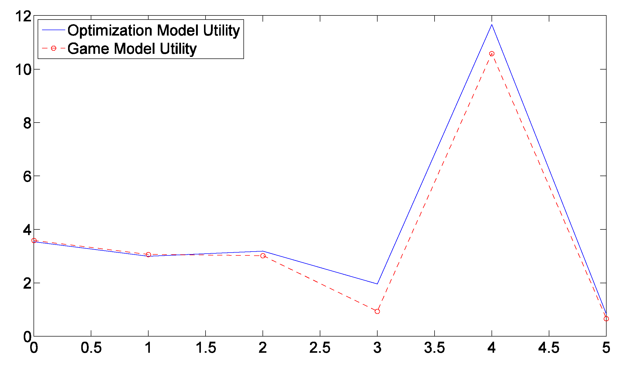
Figure 1. (a) The energy resource consumption functions; (b) technique pollution functions.
Sustainability 12 02326 g001
Figure 2. (a) The optimal energy resource use paths; (b) antipollution strategies.
Sustainability 12 02326 g002
Figure 3. (a) The game energy resource use paths; (b) antipollution strategies.
Sustainability 12 02326 g003
Figure 4. (a) The pollution paths of the multi-competitive-region model; (b) the game model.
Sustainability 12 02326 g004
Figure 5. A comparison of utility between the multi-competitive-region model and the game model.
Sustainability 12 02326 g005
Table 1. A comparison of utility between the multi-competitive-region model and the game model.
DistrictPart 1Part 2Part 3Part 4Linear SumTotal Utility
Model
The Multi-Competitive-Region Model35.341229.911131.863319.5866116.70220.8393
The Game Model35.835630.549330.11549.2892105.78940.6571
Difference between the two models−0.4944−0.63821.747910.297410.91280.1822

