Article

Utilizing Bivariate Climate Forecasts to Update the Probabilities of Ensemble Streamflow Prediction

1
Han River Flood Control Office, Ministry of Environment, Seoul 06501, Korea
2
Earth System Research Division, National Institute of Meteorological Sciences, Jeju 63568, Korea
3
International School of Urban Sciences, University of Seoul, Seoul 02504, Korea
*
Author to whom correspondence should be addressed.
Sustainability 2020, 12(7), 2905; https://doi.org/10.3390/su12072905
Submission received: 6 March 2020 / Revised: 3 April 2020 / Accepted: 4 April 2020 / Published: 6 April 2020
(This article belongs to the Special Issue Sustainable Water Resources Management for Disaster Risk Reduction)

Abstract

:
In order to enhance the streamflow forecast skill, seasonal/sub-seasonal streamflow forecasts can be post-processed by incorporating new information, such as climate signals. This study proposed a simple yet efficient approach, the “Bivar_update” model that utilizes bivariate climate forecast to update individual probabilities of the ensemble streamflow prediction. The Bayesian updating scheme is used to update the joint probability mass function derived from historic precipitation and temperature data sets. Thirty-five dam basins were used for the case study, and the modified Tank model was embedded into the ensemble streamflow prediction framework. The performance of the proposed approach was evaluated through a comparison with a reference streamflow forecast model, the “Univar_update” model, that reflects only precipitation forecast, in terms of deterministic and categorical streamflow forecast accuracy. For this purpose, multiple cases of probabilistic precipitation and temperature forecasts were synthetically generated. As a result, the Bivar_update model was able to decrease the errors in forecast under below-normal conditions. The improvements in forecasting skills were found for both measures; deterministic and categorical streamflow forecasts. Since the proposed Bivar_update model reflects both precipitation and temperature information, it can compensate low predictability especially under dry conditions in which the streamflow’s dependency on temperature increases.

1. Introduction

Accurate seasonal/sub-seasonal streamflow forecasts enable water resource agencies to formulate proper management plans for water resources, such as flood prevention (e.g., [1,2,3]), drought mitigation (e.g., [4,5]), and reservoir operation (e.g., [6,7]), for instance. In terms of the seasonal/sub-seasonal streamflow forecast model, the ensemble streamflow prediction (ESP) technique [8] has been prevalent over the past decades [9,10,11,12,13,14]. A key motivation to use the ESP approach is that it accounts for the impact of uncertainty in future meteorological forcings (such as precipitation and temperature) on the evolution of the presumably better-known watershed initial hydrological conditions. In general, the sequences of future meteorological forcings are drawn from historical traces during the prediction period. Thus, the hydrological model runs with sampled alternate climate inputs to generate an ensemble of simulated streamflow forecasts.
In order to enhance forecast accuracy, streamflow forecasts can be post-processed by incorporating new information, such as climate signals. Ensemble “trace weighting” is one of the most well-known approaches for post-processing the ESP forecasts, and its first usage was motivated by the desire to incorporate a future climate prediction signal into the ESP forecasts wherein the ensemble forecast meteorology is sampled from historical meteorological sequences [15]. Thus, the probabilities assigned to each individual forecast trace can be updated if additional climate information is given. Kelmane et al. [16] and Faber and Stedinger [17] discussed how the probabilities of individual climate traces can be updated from the Bayes theorem. Krzysztofowicz [18] and Kerr and Krzysztofowicz [19] argued that the conditional distribution of future streamflow can be derived from the Bayesian approach, given the climate forecast information.
The National Weather Service (NWS) of the National Oceanic and Atmospheric Administration (NOAA) provides an end-to-end Hydrologic Ensemble Forecast Service extending hydrologic ensemble services from six-hour to year-ahead forecasts [20]. Although an ensemble forecast can help capture the spread due to inherent uncertainty in hydrologic forecast, its predictability becomes less accurate when the forecast lead-time increases and initial conditions of the ensemble forecast are not reliable. The uncertainty of climate forecasts becomes large especially in a region wherein precipitation variability is high. Therefore, the updated probabilities on individual streamflow forecasts may not be able to enhance forecast accuracy unless the reliability of the given climate forecasts is guaranteed.
Nonetheless, there has been a growing need for using climate forecast data sets to improve streamflow forecast accuracy. A number of studies have utilized teleconnections such as El Niño–Southern Oscillation and Pacific Decadal Oscillation (e.g., [14,21]) or weather forecasts obtained from global climate models (e.g., [22]). However, in terms of weather forecasts, studies tend to utilize only precipitation forecasts despite great uncertainty in precipitation forecasts (e.g., [23,24]). Understandably, their argument in defense of the use of precipitation forecast is based on the fact that runoff sensitivity to precipitation is generally greater than temperature, and consequently, temperature forecasts are easily overlooked. However, the runoff sensitivity to temperature increases under a dry climate regime or in a low water season [25]. Shukla et al. [26] also argued that the role of temperature plays an important role especially under drought conditions. It must be noted that cross-correlation between precipitation and temperature can potentially impact streamflow simulations [27]. Scheuerer et al. [28] discussed that interdependency between precipitation and temperature must be reconstructed to physically generate realistic forecast trajectories. Chen et al. [29] also emphasized the advantage of correcting cross-correlation between precipitation and temperature of climate model outputs on hydrological modeling. Additionally, climate forecast models generally employ a mathematical model of the general circulation of a planetary atmosphere or ocean such as a general circulation model (GCM). The atmospheric models, which are coupled in GCMs calculate multiple variables such as winds, heat transfer, radiation, relative humidity, and surface hydrology so that precipitation and temperature series can be calculated simultaneously by a system of differential equations. Given that climate forecasts are obtained using a physical-based climate model, the cross-correlation between precipitation and temperature would propagate to pairs of precipitation and temperature forecast data sets [30].
With the purpose of enhancing the streamflow forecast performance, this study aims to (i) propose an efficient and simple approach that utilizes bivariate climate forecast information to update the probabilities of ensemble streamflow forecasts. The proposed methodology is described in the following ‘Theoretical background’ section. Regarding climate forecast information, both precipitation and temperature forecasts are employed to update streamflow forecasts probabilities. The current probabilistic climate forecast system of Korea is introduced in the ‘Case study’ section along with the data sets used in this study. Furthermore, (ii) the performance of the proposed approach is evaluated through its comparison with a reference approach that utilizes precipitation forecast solely in terms of deterministic and categorical forecast verification measures. In Section 3.5 the overall evaluation framework illustrates the modeling setting for the performance evaluation of the proposed method. Moreover, (iii) skill performance is evaluated under below-normal conditions in order to address the role of temperature in improving streamflow predictability under drought conditions. Overall, results are demonstrated in the ‘Results’ section followed by the ‘Discussions and Conclusions’ section.

2. Theoretical Background

2.1. Ensemble Streamflow Prediction

Ensemble streamflow prediction (ESP; [8]) is a widely used method for probabilistic forecasting in operational hydrology [31]. ESP runs a rainfall-runoff model with observed meteorological inputs to generate an ensemble of possible runoff (or streamflow) hydrographs [10,13,14]. In the ESP technique for mid- and long-range lead-time, all the historical meteorological scenarios are typically inserted into a rainfall-runoff model under the underlying assumption that they are likely to occur in the future. Since the initial conditions of the rainfall-runoff model vary depending on the time of the forecast, the ensemble streamflow forecasts vary as per the initial conditions. The initial conditions present for each point of forecast time are set up by executing the rainfall-runoff model with the observed forcing datasets for a certain length of spin-up period (the previous five years, for instance). As a result, the generated ensemble of streamflow forecasts is also a function of the current hydrological conditions driven by the rainfall-runoff model. Therefore, this technique is often called a “conditional Monte Carlo simulation approach” [8].

2.2. Croley-Wilks Approach

Croley [32,33] and Wilks [34] posited that the conditional distribution function P[g(v)|D] is summarized by the probability of the selected set of climate variables g(v), which falls into the three intervals: below-normal, normal, and above-normal. The climate information utilized to determine the conditional distribution is symbolized by D. Their algorithm adjusts the probabilities assigned to the different traces so as to achieve the target probabilities using the values of the selected variables, g(vi), but only to the extent that they determine whether a given climate series, vi, falls into the below-normal, normal, or above-normal range for g(vi) [35]. Following the non-parametric approach developed by Croley [32] and Wilks [34], which assigned the same probability to climate scenarios included in each category, Stedinger and Kim [35] proposed a simple and general approach, the PDF-ratio approach. This approach utilized the entire P[g(v)|D] distribution as well as the individual values of the selected variables, g(vi), associated with each vi to generate series-probability pairs {(vi, qi)}. These pairs provided a better approximation of the entire P[g(v)|D] distribution. Nonetheless, there was no significant difference in the accuracy of updated streamflow forecasts between the Croley–Wilks approach and PDF-ratio approach [36]. Eventually, the Croley–Wilks approach was adopted in this study due to its easy implementation and the format of climate forecast data sets, which is described in Section 3.2.

2.2.1. Definition of Three Interval Probabilities

Consider a set of historical climate scenarios including two random variables defined as a vector ( x i , y i )   for   i = 1 ,   2 ,     N . X and Y are random variables of monthly precipitation and temperature respectively that have quantiles x b and x a such that 0.333 = F ( x b ) = F ( x a ) F ( x b ) = 1 F ( x a ) and y b and y a such that 0.333 = F ( y b ) = F ( y a ) F ( y b ) = 1 F ( y a ) where F ( · ) is an empirical cumulative distribution function. x a ( y a ) and x b ( y b ) are the upper and lower terciles of monthly precipitation (temperature) series respectively, defining above-normal, and below-normal ranges.
Given the terciles x a and x b , let us assume that the probabilistic precipitation forecast (PPF) is given as,
F ( x b ) = p x , b ,
F ( x a ) F ( x b ) = p x , n ,
1 F ( x a ) = p x , a ,
where
p x , b + p x , n + p x , a = 1
The three interval probabilities, p x , b ,   p x , n , and p x , a , are defined as below-normal, normal, and above-normal probabilities respectively. Likewise, the three interval probabilities, p y , b ,   p y , n , and p y , a . The below-normal, normal, and above-normal probabilities as a form of probabilistic temperature forecast (PTF) can be obtained with the terciles y a and y b .

2.2.2. Utilizing Univariate Climate Forecast Information

To utilize climate forecast information such that the prior probabilities, 1/N, on the   x i can be updated to new probabilities, the Croley–Wilks approach [32,33,34] was adopted in this study. Croley and Wilks developed a probability adjustment technique that assigns the same probability to the climate scenarios in each selected interval [32,33,34]. The procedure of the utilizing univariate climate forecast information—probabilistic precipitation forecast in this study—is described in Appendix A.

2.2.3. Utilizing Bivariate Climate Forecast Information
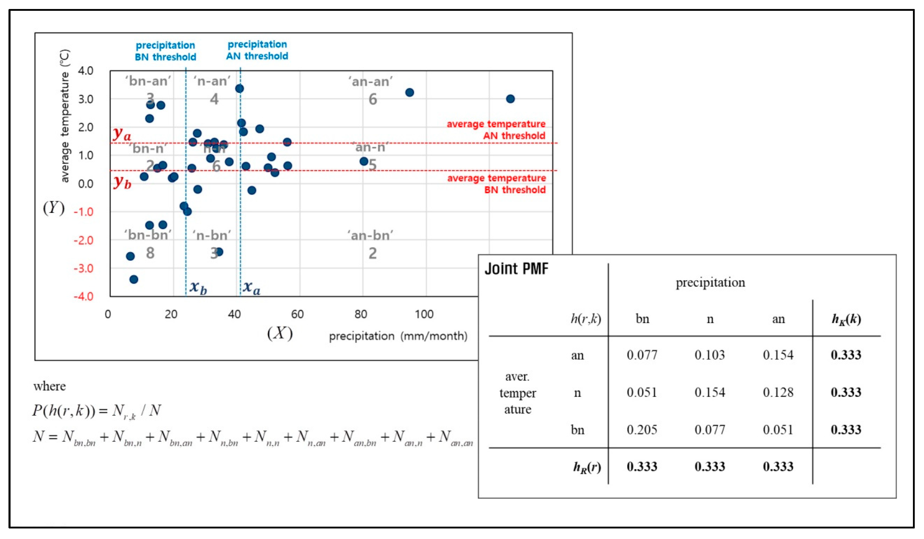
To utilize bivariate climate forecast information, a joint probability mass function describing the PPF and the PTF was adopted in this study. Since both PPFs and PTFs are discrete random variables provided as a form of three interval probabilities, their simultaneous behavior can be described with a joint probability mass function (PMF). Let us define the joint probability mass function as Equation (5),
h ( r , k ) = H ( R = r , K = k )
where R and K are discrete random variables having three interval values, bn, n, and an for monthly precipitation and temperature respectively.
First, in order to obtain a reference joint PMF, H , historic observation pairs of X and Y are classified into nine categories. The categories are divided based on the upper and lower terciles of both monthly precipitation and temperature series, so they are named bn–bn (when both precipitation and temperature are below-normal), bn–n (when precipitation is below-normal and temperature is normal), an–n (when the precipitation is above-normal and temperature is normal), and an–an (when both precipitation and temperature are above-normal), and so on. The joint PMF can thus be empirically calculated as Equation (6),
P ( H ) = P ( h ( r , k ) ) = N r , k / N ,
where N r , k refers to the number of scenarios when X is in r interval and Y is in k interval and N is the number of all the historic scenarios.
Figure A1 in Appendix B demonstrates how to obtain the reference joint PMF with historic climate data sets. The P ( h ( r , k ) ) thus becomes the prior PMF.
To obtain the likelihood function, the PPF and the PTF for the current forecast time are utilized. With the assumption that the probability on each tercile interval provided by the PPF and the PTF, that is, [ p x , b ,   p x , n , p x , a ] and [ p y , b ,   p y , n , p y , a ] is the probability of detection of that interval, the likelihood function can be calculated as Equation (7), with the assumption that PPFs and PTFs are independent. In Monsoon climate regions such as South Korea, cross-correlations between temperature and precipitation exist in summer and winter seasons although the relationships are often statistically not significant. This study adopted the assumption of independence between temperature and precipitation forecasts for easy implementation of the proposed method
P ( D | H ) = P ( D | h ( r , k ) ) = p x , r · p y , k     r = b n , n , a n   k = b n , n , a n ,
Figure A2 in Appendix B demonstrates how to obtain the joint PMF for the current forecast based on the PPF and the PTF. The posterior PMF is then calculated using the Bayesian updating scheme, which is based on the Bayes’ theorem and the total probability rule. With discrete priors, the posterior PMF is calculated as Equation (8),
P ( H | D ) = P ( h ( r , k ) | D ) = P ( D | h ( r , k ) ) P ( h ( r , k ) ) P ( D )   ,
where P ( D ) = r k P ( D | h ( r , k ) ) P ( h ( r , k ) ) = r k ( p x , r · p y , k ) ( N r , k / N ) .
Figure 1 demonstrates an example calculation of a posterior PMF updated by a prior PMF and a likelihood function. Given that the posterior joint PMF is provided as a form of nine categorical probabilities (as presented in Figure 1), prior probabilities on each historical climate scenario, 1 / N , are simply updated as Equation (9),
P ( h ( r , k ) | D ) / N r , k       r = { b , n , a } ,     k = { b , n , a } ,
where N r , k is the number of historical climate scenarios that belong to r interval for precipitation and k interval for average temperature.
Based on the adjusted probabilities of the climate scenarios in each category (i.e., posterior joint PMF), the ensemble mean of streamflow forecast, μ q , is calculated as Equation (10),
μ q = r k μ q r , k ,
where
  • μ q b , b = ( P ( h ( b , b ) | D ) / N b , b ) q i   ( only   when   x i x b   and   y i y b ) ,
  • μ q n , b = ( P ( h ( n , b ) | D ) / N n , b ) q i   ( only   when   x b < x i x a   and   y i y b ) ,
  • μ q a , b = ( P ( h ( a , b ) | D ) / N a , b ) q i   ( only   when   x a x i   a n d   y i y b ) ,
  • μ q b , n = ( P ( h ( b , n ) | D ) / N b , n ) q i   ( only   when   x i x b   and   y b < y i y a ) ,
  • μ q n , n = ( P ( h ( n , n ) | D ) / N n , n ) q i   ( only   when   x b < x i x a   and   y b < y i y a ) ,
  • μ q a , n = ( P ( h ( a , n ) | D ) / N a , n ) q i   ( only   when   x a x i   and   y b < y i y a ) ,
  • μ q b , a = ( P ( h ( b , a ) | D ) / N b , a ) q i   ( only   when   x i x b   and   y a y i ) ,
  • μ y n , a = ( P ( h ( n , a ) | D ) / N n , a ) q i   ( only   when   x b < x i x a   and   y a y i ) ,
  • μ y a , a = ( P ( h ( a , a ) | D ) / N a , a ) q i   ( only   when   x a x i   and   y a y i ) and q i is simulated streamflow driven by the ith climate scenario (i.e., q i is a function of x i and y i ).
Here, if a constant (uniform) prior, that is, all the P(h(r,k)) equal to 0.111 (=1/9) are given no observation, is available, then, posterior PMF becomes equal to the likelihood which is new information based on the categorical forecast.

2.3. Performance Evaluation Metrics

RMSE is frequently used to measure the differences between values predicted by a model and observed values. In this study, the normalized-root mean squared error (NRMSE) was used to evaluate the quantitative error between the observed and predicted values. The normalizing of RMSE facilitates a comparison between data sets with different scales (different mean values of monthly streamflow across all the season, for instance).
Additionally, the probability of detection (POD) is used to evaluate the accuracy of categorical forecasts. The POD is a ratio indicating the frequency of an event that occurred on the date it had been forecast to occur [37]. In this study, a 3 × 3 contingency table for the categorical forecast verification situation was used as shown in Figure A3 in Appendix C. The categories were divided into below-normal, normal, and above-normal, with x a o b s and x b o b s as the upper and lower terciles of observations. The total for each of the nine possible forecast and event pair outcomes are denoted by the letter a through i. The POD is given by the proportion of correct forecasts (denoted as “hit” in the contingency table), that is, in the 3 × 3 contingency table represented in Figure A3 in the Appendix C, the POD would be (a+e+i)/(a+b+c+d+e+f+g+h+i).

3. Case Study

3.1. Application Sites and Data Sets

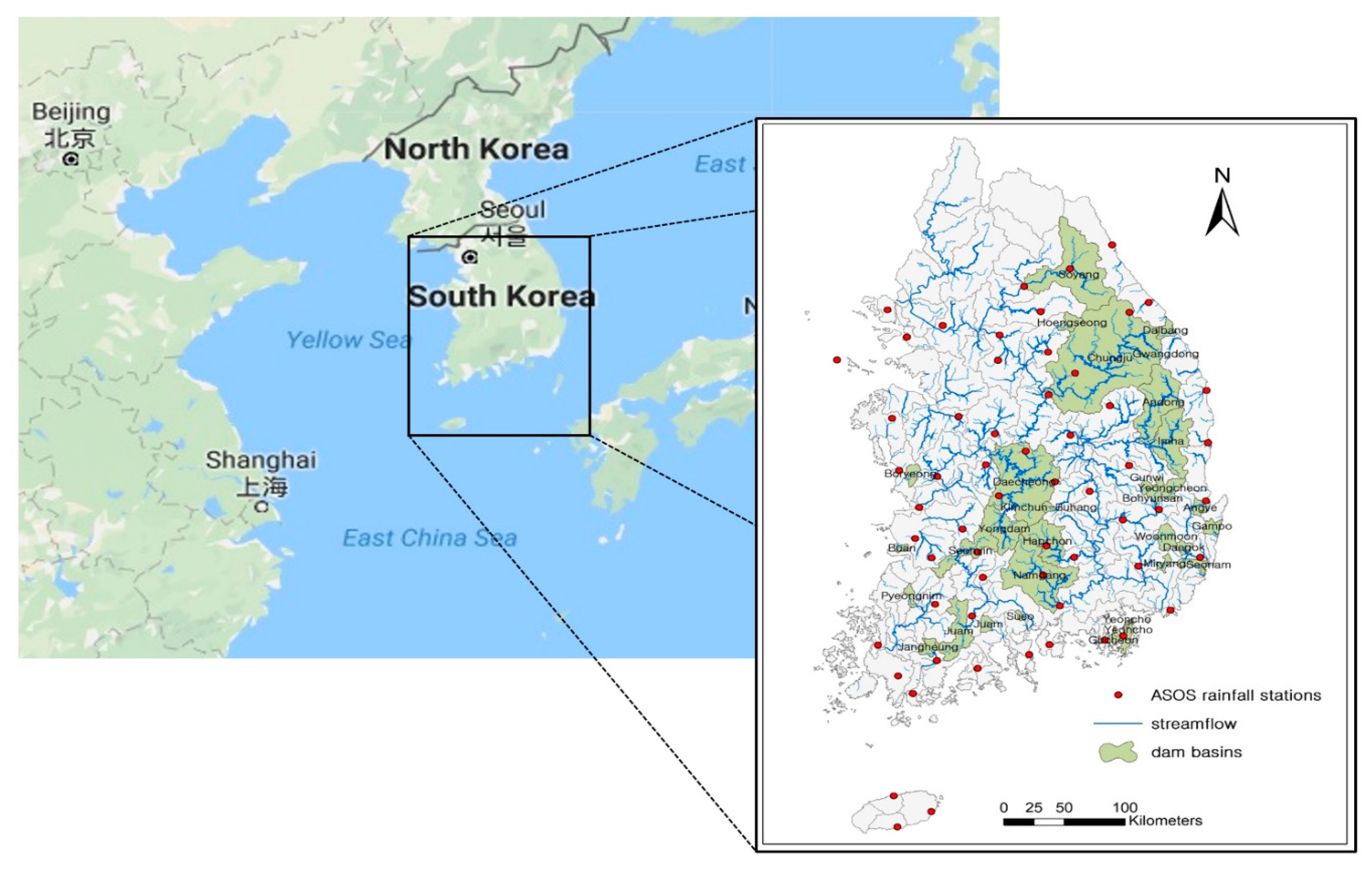
This study includes 35 watersheds wherein dams are operated below the watershed outlet. Table 1 presents a list of the 35 watersheds used in this study, while Figure 2 depicts the locations of the watersheds across South Korea. South Korea has a distinct seasonality in precipitation and temperature. Winters are usually cold and dry, while summers are very hot and humid. The climatic regime is dominated by the Asian monsoon; thus, approximately 66% of total annual precipitation and runoff occur during the wet summer that spans from July to September. Monsoons form the major driver behind the magnitude, timing, and distribution of wet season rainfall, rainfall interannual variability, and rainfall extremes in this region. On the other hand, the dry season spans from November to April. The daily observed streamflow (dam inflow) series from 1966 to 2016 at 35 dam sites were collected from the K-water Institute. Observed meteorological data sets from 1966 to 2016—daily precipitation, maximum/minimum temperature, and average wind speed series—were collected from 60 Automated Synoptic Observing System (ASOS) locations of the Korea Meteorological Administration (KMA). Daily potential evapotranspiration series were estimated by the FAO Penman-Monteith equation No. 56 method [38]. These data sets were converted into mean areal values for each test watershed using the Thiessen Polygon method [39].

3.2. Probabilistic Climate Forecast

In a practical hydrologic forecasting system of Korea, The KMA provides climate forecast as a form of simple probability mass function, which refers to the application of cutting edge technologies to predict the atmosphere state on a given location for the near future. Since May 2014, KMA has been operationally running climate prediction system named GloSea5 (Global Seasonal Forecasting System version 5) which is the joint seasonal forecasting system with the UK Met Office [40]. The atmospheric initial conditions come from KMA’s 4D-VAR system. KMA has been reporting mid- and long-range probabilistic forecasts to the public for 12 provinces of the Korean Peninsula. The mid-range forecast produces one-week-ahead precipitation and maximum/minimum temperature on a daily basis. On the other hand, long-range forecast reports one-month and three-month outlooks for precipitation and average temperature on a weekly and monthly basis, respectively, as a discrete form of probability for each tercile interval: below-normal, normal, and above-normal. Figure 3 illustrates an example of the three-month outlook for the precipitation and average temperature probabilities that are reported on a monthly basis. As shown in Figure 3, the probability for each tercile interval is the forecast.

3.3. Realization of Synthetic Climate Forecasts

To evaluate the role of climate probabilistic forecasts on the accuracy of the ESP, multiple sets of the PPF and the PTF were synthetically generated. The synthetic probabilistic forecast sets were sampled from historical forecasts. Using the target value of the POD that ranges from 0.3 to 1.0 increasing by a 0.1 interval, synthetic sets of PPFs and PTFs were generated for each province. The two steps used for generating the synthetic probabilistic forecasts are described in Appendix D.

3.4. Rainfall-Runoff Model

A modified conceptual rainfall-runoff model (Tank model with soil moisture structure) was used as a deterministic hydrologic model for the runoff simulation. With four tanks and a soil moisture structure, the Tank model simulates the net stream discharge as the sum of discharges from the side outlets of the tanks [41]. In order to consider the snow accumulation-melting module, the modified Tank model developed by McCabe and Markstrom [42] was used. The daily time series of the precipitation, temperature, and potential evapotranspiration were used as input data. If the temperature is below the value of the specified threshold ( T s n o w ), all forms of precipitation are considered to be snow. If the temperature is higher than the value of the additional threshold ( T r a i n ), all forms of precipitation are considered to be rain. Within the range defined by T s n o w and T r a i n , the amount of precipitation becoming snow decreases linearly from 100 to 0 percent of the total precipitation. This relation is expressed as Equation (11),
P s n o w = P × [ T r a i n T T r a i n T s n o w ]   ,
P r a i n is computed as P r a i n = P P s n o w . For the snowmelt module, the fraction of snow storage (snostor) that melts in a month (snowmelt fraction, or SMF) is computed through the mean monthly temperature (T) and the maximum melt rate (meltmax). meltmax is often set to 0.5 [43]. SMF is computed as Equation (12),
SMF = T T s n o w T r a i n T s n o w × m e l t m a x ,
If the computed SMF is greater than meltmax, then SMF is set to meltmax. The amount of snow melted in a month (SM) is computed as SM = s n o s t o r × SMF .
The parameters of the model were estimated using the shuffled complex evolution algorithm, a population–evolution-based global optimization method [44]. Seo and Kim [45] provide an informative schematic diagram of the Tank model. The Tank model parameters for the target watersheds were calibrated and validated by a previous study [45]. The NSE values for the 35 watersheds ranged from 0.68 to 0.91, and the Percent bias values ranged from –1.57 to 8.93.

3.5. Overall Evaluation Framework

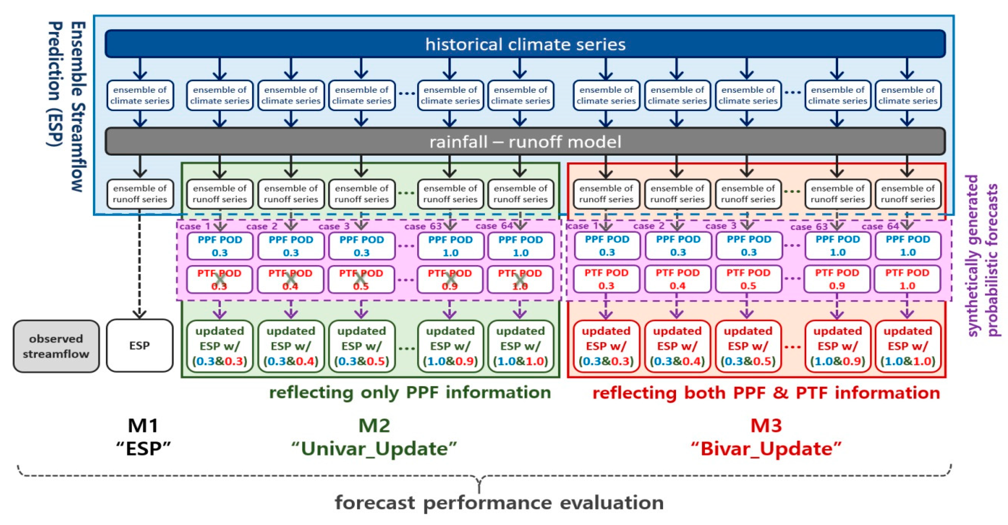
Figure 4 comprises of an overall evaluation framework for this study, illustrating a way of assessing the impacts of the proposed approach that incorporates bivariate climate information on the ESP. First, the one-month-ahead streamflow forecasts are obtained by the ESP. All the boxes in the ESP diagram (blue box in Figure 4) are the same ensemble forecast sets to be updated. The results of the ESP (ensemble mean of simulated runoff scenarios) are updated with a set of synthetic probabilistic forecast i) using the Croley–Wilks-based approach utilizing only the PPF information (green box in Figure 4, hereinafter ‘Univar-update’) and ii) using the proposed approach utilizing the PPF as well as the PTF information (red box in Figure 4, hereinafter ‘Bivar-update’). The updated streamflow forecasts outputs were then evaluated through comparison with the observed streamflow series. By comparing the performance between traditional ESP and the Univar-update (M1 versus M2 in Figure 4), the impact of utilizing the precipitation forecast information on the accuracy of the ESP can be evaluated. By comparing the performance between Univar-update and Bivar-update (M2 versus M3 in Figure 4), the relative improvement in the ESP accuracy can be evaluated when both precipitation and temperature forecast information are incorporated as compared to utilizing precipitation solely.
The application period of this study is from January 1971 to December 2013. The generation of synthetic probabilistic forecast pairs is repeated hundred times for each POD combination case (PPF POD—PTF POD pair) such that the total number of synthetic probabilistic forecast pairs is 6400 sets (100 sets × 64 POD combination case).

4. Results

4.1. Deterministic Forecast Evaluation

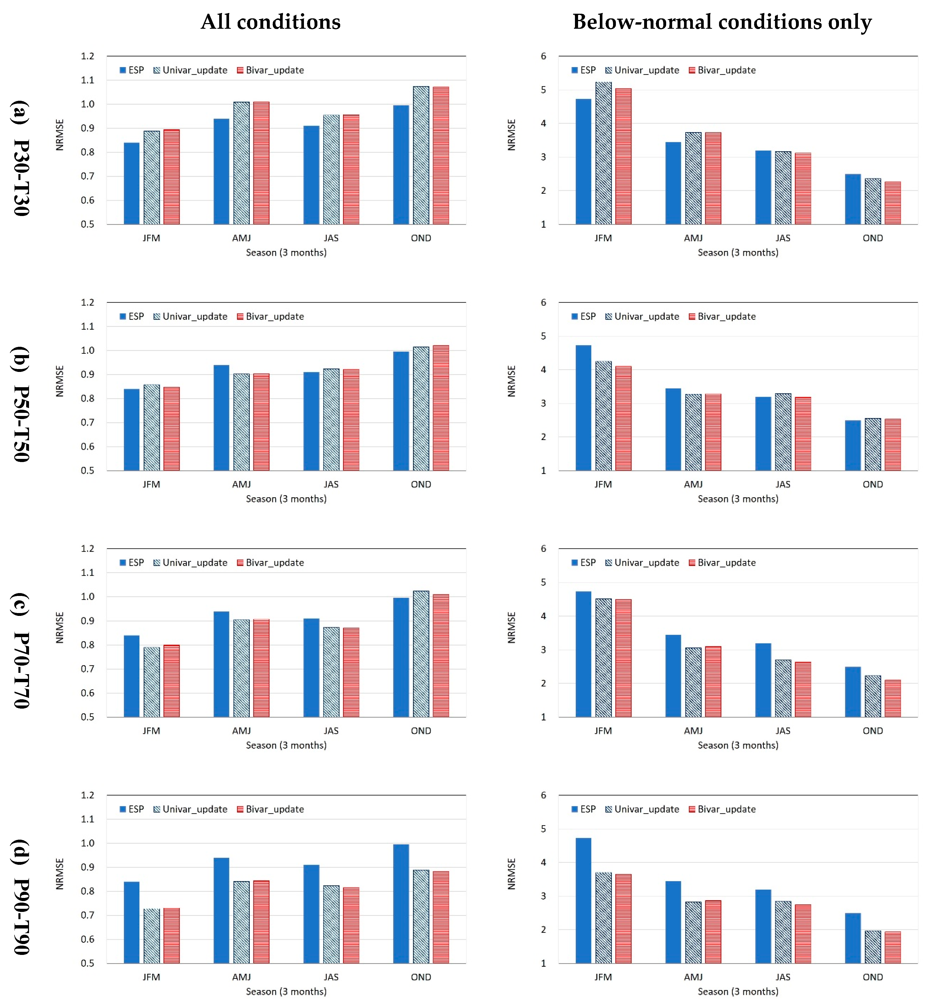
In order to evaluate deterministic forecast accuracy, the ensemble mean of three forecasting models—ESP, Univar_update, and Bivar_update—was estimated for the historic period. The NRMSE for the three models was then calculated by comparing the observed values. For both Univar_update and Bivar_update models, 64 cases of synthetic probabilistic forecasts series were applied. In Figure 5, NRMSE values for four seasons—JFM (Jan.–Mar.), AMJ (Apr.–Jun.), JAS (Jul.–Sep.), OND (Oct.–Dec.)—were presented, and the presented values constitute the mean NRMSE across 35 basins. Among the 64 cases of synthetic probabilistic forecasts, four selected cases—30% POD for PPF and 30% POD for PTF (P30–T30), 50% POD for PPF and 50% POD for PTF (P50–T50), 70% POD for PPF and 70% POD for PTF (P70–T70), 90% POD for PPF and 90% POD for PTF (P90–T90) are presented in Figure 5.
As depicted in Figure 5a, when the synthetic probabilistic forecasts skill is low (i.e., P30–T30), the forecasting errors arising in both updating approaches were greater than the ESP. When the POD of probabilistic climate forecasts is lower than climatology (33.33% of POD), the impact of utilizing climate information on streamflow forecast was understandably negative. The difference between the two updating models—Univar_update and Bivar_update—was not distinct, although the errors in the Bivar_update model were slightly less than those in the Univar_update under the below-normal conditions.
However, as depicted in Figure 5b–d, as the synthetic probabilistic forecasts skill improves, positive impacts of utilizing climate information on streamflow forecast accuracy were found. When the POD of probabilistic climate forecasts is 90% (Figure 5d), the difference between the ESP and the two updating models was presented. This clearly demonstrates that the two updating approaches can enhance streamflow-forecasting skill when reliable climate forecast information is provided. On the other hand, no significant difference was found between two updating models in terms of NRMSE values regardless of probabilistic climate forecasts skills. Nonetheless, the Bivar_update generally returned lesser values in NRMSE than Univar_update, especially under below-normal conditions and JAS season. It relates to the sensitivity of the climate variables to streamflow under below-normal conditions. A below-normal condition implies a lack of water on the atmosphere and surface such that the sensitivity of temperature to streamflow increases due to increased impact of evaporation. JAS season constitutes summer in Korea, so the impact of evaporation on streamflow is greater during JAS season than other seasons. Under this circumstance, it can be induced that incorporating the temperature forecast information can enhance streamflow forecast performance given that the temperature forecast skill is reliable.
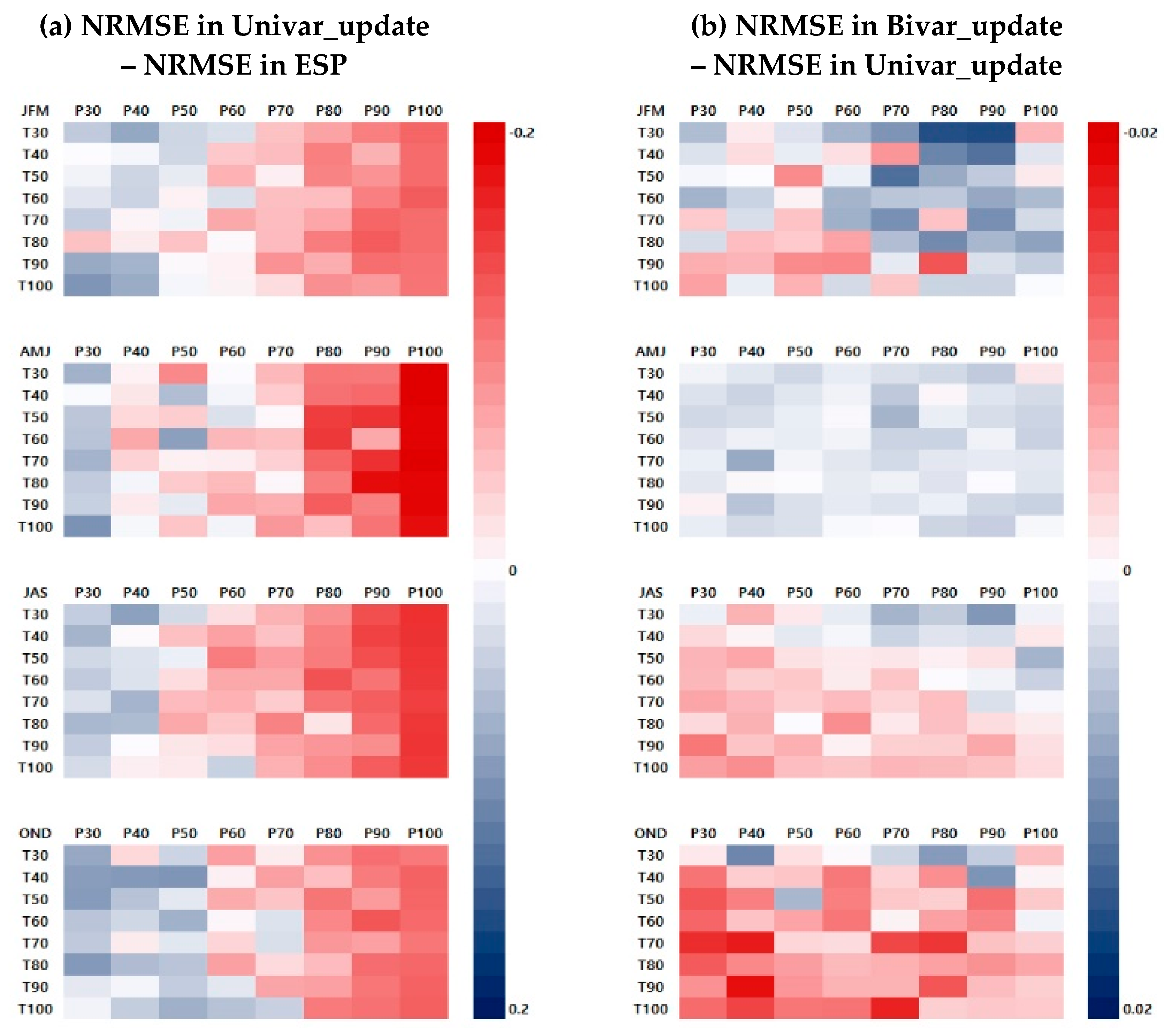
Figure 6 compares errors in streamflow forecasts across all 64 cases of synthetic probabilistic forecasts. In Figure 6a, the differences in NRMSE values between the Univar_update and the ESP are presented for four different seasons. The negative value (red color in cells) represents that the Univar_update has better prediction skill than the ESP. As the PPF skill increased, the NRMSE in the Univar_update indisputably continued to decrease. A strong horizontal gradient can be seen across seasons. It was noted that NRMSE values in the ESP remain the same across all cells. In addition, since the PTF was not utilized in the Univar_update, little differences in NRMSE across vertical lines of the Univar_update model were caused by the inherent randomness of the synthetic climate forecast generation scheme. On the other hand, Figure 6b depicts differences in NRMSE values between the Bivar_update and the Univar_update. The negative value (red color in cells) demonstrates that the Bivar_update has smaller errors. A vertical gradient can be seen across seasons although it is not particularly discernable in AMJ. This can be expected because the Bivar_update utilizes PTF information to update streamflow forecast. Moreover, the lower the value of the POD given for the PPF, the greater is the vertical gradient presented. In Figure 6b it is found that there is seasonal pattern of the skill difference between the two models. The reason the skill difference is negligible in AMJ season might because there is relatively high variability in precipitation. On the other hand, the skill improvement by Bivar_update model in JAS season can be explained by the strong streamflow dependency on temperature. Although, JAS season shows the most variability in precipitation, the Bivar_update model can compensate this uncertainty when the skill of temperature forecast is sufficiently high (e.g., P30~P40 & T90~T100 combinations). It implies that the Bivar_update can compensate the low skill of PPF when the PTF skill is greater than the PPF skill. Temperature forecasting skill is generally better than precipitation forecasting in practical climate forecasting due to greater uncertainty in precipitation. In this light, the utilization of temperature forecast information should not be overlooked.
Figure 7 compares the errors in streamflow forecasts only under a below-normal condition across the 64 cases of synthetic probabilistic forecasts. Figure 7a depicts a horizontal gradient pattern, which implies that the greater the POD values of PPF, the better is the improvement of streamflow prediction by the Univar_update. On the other hand, almost all the cells have red colors in Figure 7b, which implies that the Bivar_update outperformed the Univar_update across all 64 cases of synthetic probabilistic forecasts (although the differences are not distinct in AMJ). Under dry conditions, it was found that incorporating the PTF information led to quick improvement in streamflow forecasting skill, even with moderate PTF skill, and its impact slowly increased as the POD values of the PTF increased. It should be noted that the decrement in NRMSE by the Bivar_update under a below-normal condition (Figure 7b) is quite significant as compared to the decrement in all the conditions (Figure 6b). The ratio between the color legend scale of (a) and (b) is much smaller in Figure 7 (approximately 1:3) when compared to Figure 6 (1:10). This implies that the positive impact of the Bivar_update model on streamflow prediction skill is clearly demonstrated under dry conditions. In addition, it also shows that there is distinct seasonal pattern of the skill difference between the two models under below normal conditions. Regardless of precipitation forecasting skill, during the dry climate conditions in which role of temperature on streamflow simulation increases, the performance of Bivar_update was noticeable.

4.2. Categorical Forecast Evaluation

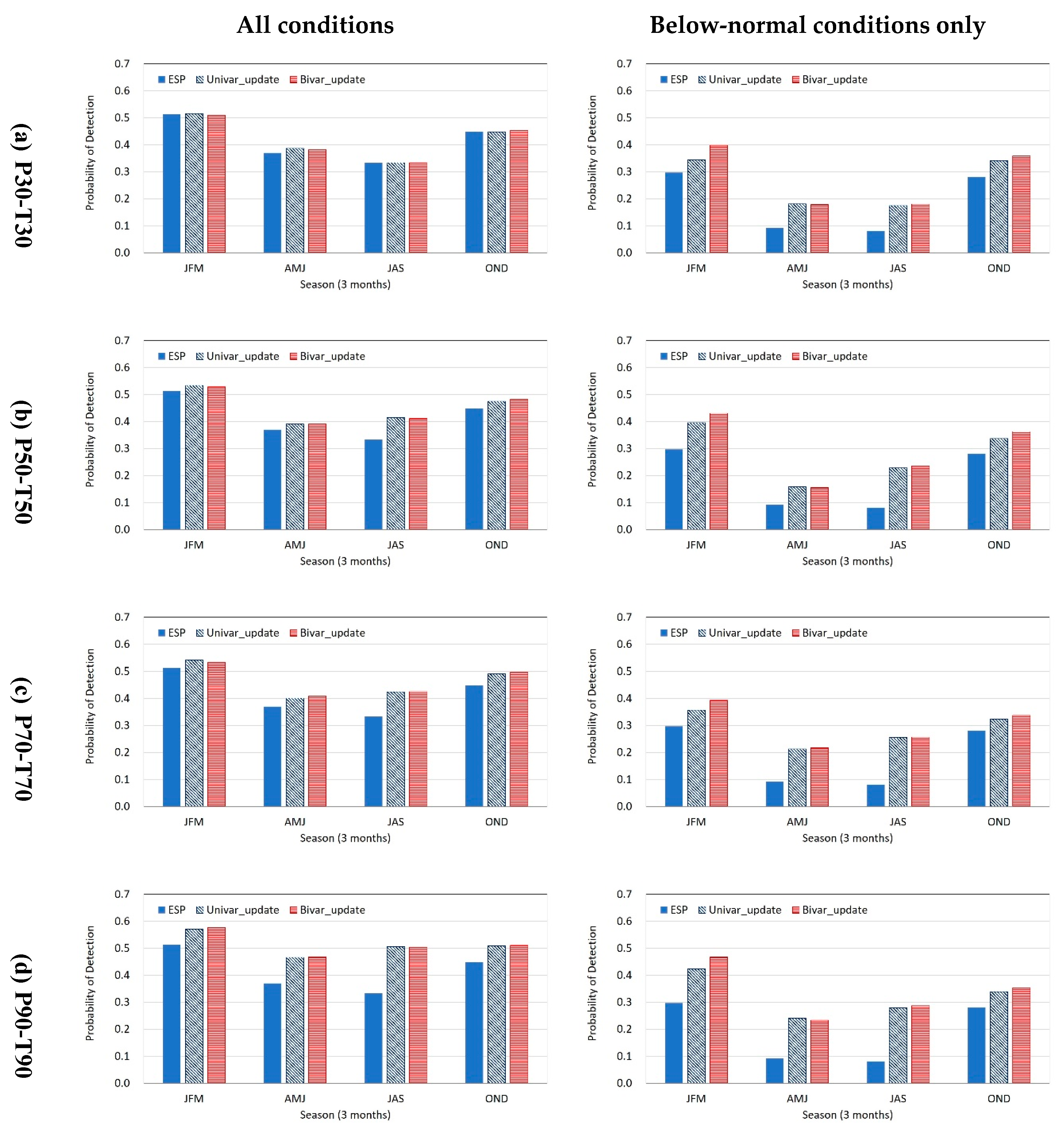
In terms of categorical forecast evaluations, the POD of categorized streamflow forecasts from the three forecasting models was estimated for historic period, and the average value of the POD across 35 basins is presented in Figure 8. As depicted in Figure 8a, the POD values of the three forecasting models were very close each other when the synthetic probabilistic forecasts skill was low (i.e., P30–T30). On the other hand, as the POD of synthetic probabilistic forecasts increased, the two updating models demonstrated greater POD values than ESP. In addition, similar to Figure 5, there were no significant differences in the POD values between the two updating models. Nonetheless, the Bivar_update clearly outperformed the Univar_update under below-normal conditions, especially in the JFM and OND seasons. Since the impact of evaporation on streamflow increases during the low flow season, it can be inferred that the Bivar_update model efficiently increased the categorical streamflow forecast skill under dry conditions. JFM and OND are low flow seasons in Korea, implying that the internal variability in streamflow is very low during those seasons. Due to lower internal variability (i.e., lower uncertainty in forecast), the POD values of the ESP were relatively significant in the JFM and OND seasons. Moreover, the impact of incorporating the PTF on streamflow prediction was greater in these seasons than other seasons.
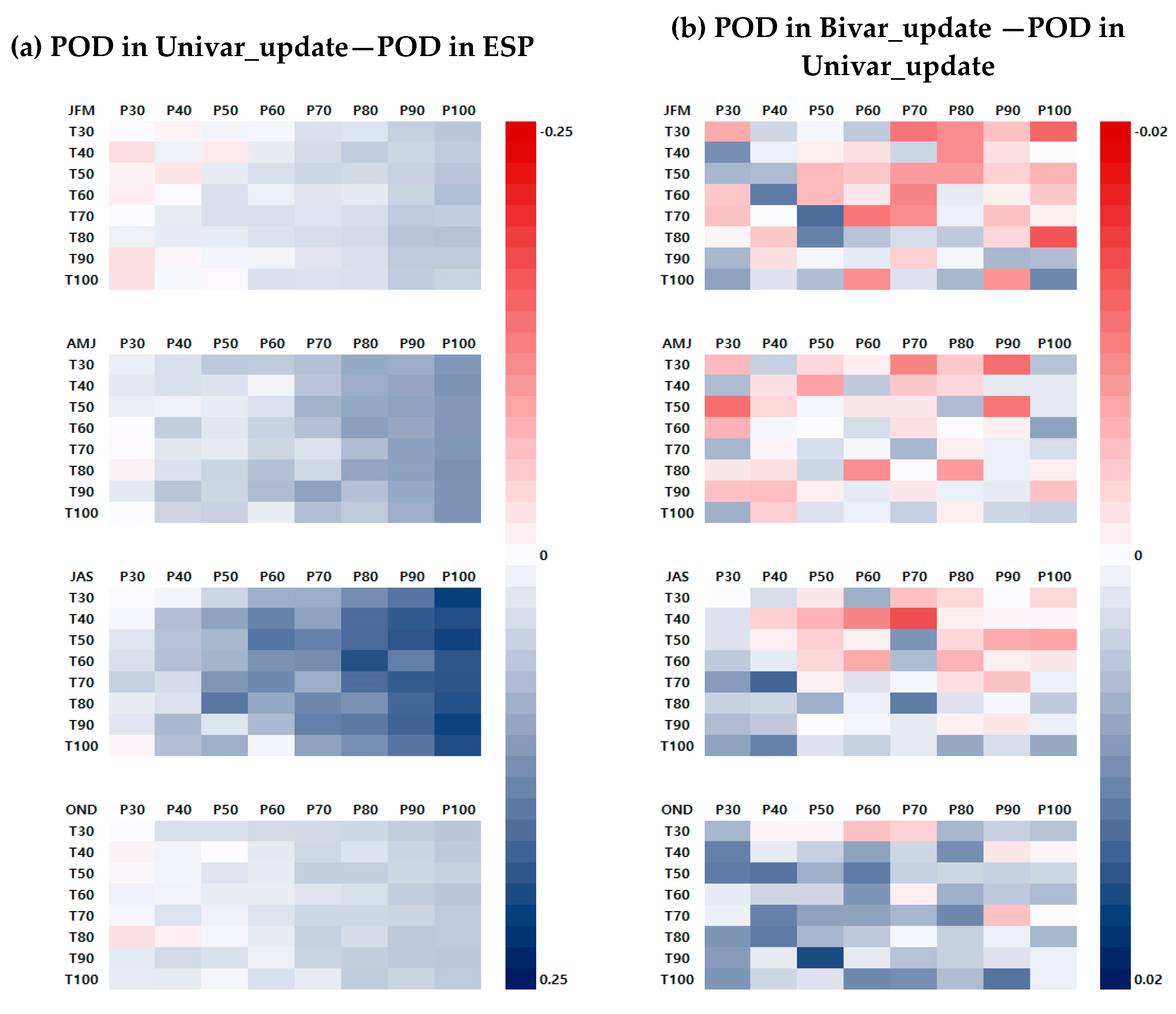
Figure 9 presents the comparison of categorical streamflow prediction skill between the three forecasting models. Unlike Figure 6a, the positive value (blue color in the cells) in Figure 9a depicts that the Univar_update has better prediction skill than the ESP. As the PPF skill increased, the POD values in the Univar_update continued to increase. As expected, a distinct horizontal gradient can be seen across all seasons. The Univar_update significantly enhanced the categorical streamflow forecast skill in JAS season as compared to other seasons. Since there is a huge inter-annual variability in streamflow in JAS season, the reference POD values (POD values from the ESP) were very low. Hence, when good PPF skill was provided, the Univar_update model significantly improved the streamflow forecast skill. Here it should be noted that this was not the case under deterministic forecast evaluation. When deterministic forecast errors are evaluated, an observed outlier leads to great penalty on the evaluation metric based on the distance between the observed and simulated value. On the other hand, when it comes to categorical forecast evaluation, no penalty is imposed on the simulated value if the simulated value is included in the same category with the observation, despite the large distance between the observed and simulated values. Therefore, a slight shift toward the observation can significantly increase the POD values (if the shift changes the forecasting category correctly).
On the other hand, Figure 9b depicts the differences in the POD values between the Bivar_update and the Univar_update. Positive value (blue color in the cells) depicts that the Bivar_update has smaller errors. A vertical gradient is clearly seen in the JAS and OND seasons, but some irregular patterns can be seen in the JFM and AMJ seasons. The Bivar_update could not increase the POD values when PPF skill was very good (around P70–P100). The Bivar_update was successfully able to enhance categorical streamflow forecasting skill only when the PPF skill was low (around P30–P60). This implies that poorly forecasted temperature information (low POD value in the PTF) can diminish the potential improvement in the streamflow forecast obtained by incorporating excellent precipitation forecast information (significant POD value in the PPF). On the contrary, it implies that reliable skill of temperature forecast can also compensate the low skill of streamflow forecast driven by poor precipitation forecast.
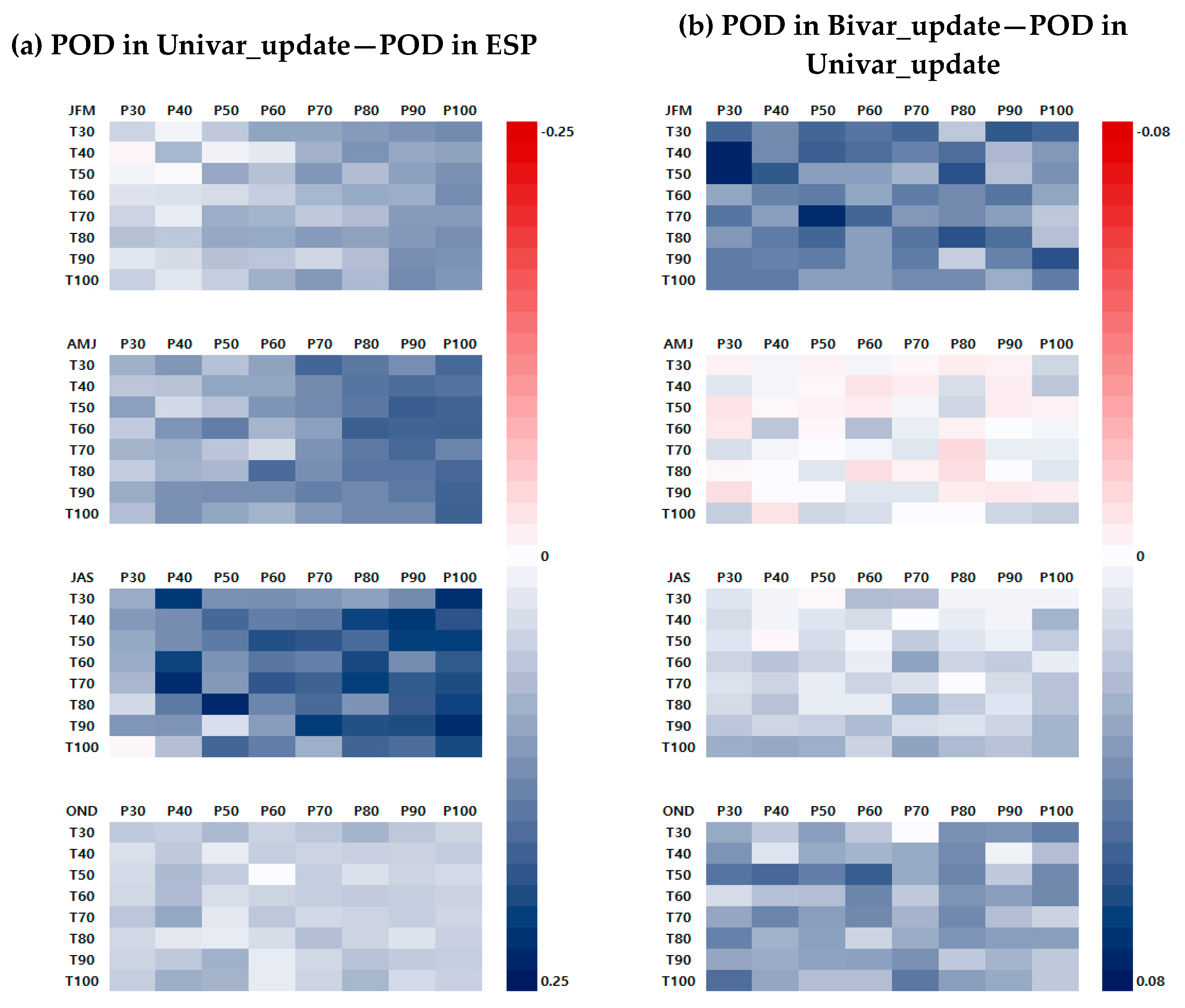
Figure 10 presents a comparison of categorical streamflow prediction skill between the three forecasting models only under below-normal conditions across the 64 cases of synthetic probabilistic forecasts. Figure 10a depicts a horizontal gradient pattern conveying that better forecasts in PPF lead to greater POD values in categorical streamflow forecasts. The increment in the POD values on streamflow forecasts was greater in AMJ and JAS seasons, when inter-annual variabilities were greater than during other seasons. Similar to the results of a deterministic forecast evaluation, the Univar_update model was able to improve the categorical streamflow forecast skill when inter-annual variability of streamflow was significant. Figure 10b presents the differences in the POD values between the Univar_update and the Bivar_update models. It clearly depicts the Bivar_update outperforming the Univar_update across all 64 cases of synthetic probabilistic forecasts except during the AMJ season. Although the superiority of the Bivar_update model over the Univar_update was not shown clearly (especially when the PPF skill was better than the PTF), the Bivar_update model outperformed the Univar_update when only the dry condition was taken into consideration. It should be noted that the increment in the POD by the Bivar_update model under below-normal conditions (Figure 10b) is quite significant when compared to the increments in other conditions (Figure 9b). The ratio between the color legend scale of (a) and (b) are much smaller in Figure 10 (approximately 0.08:0.25) when compared to Figure 9 (0.02:0.25). This implies that the superiority of the Bivar_update model on categorical streamflow prediction skill is more remarkable under dry conditions.
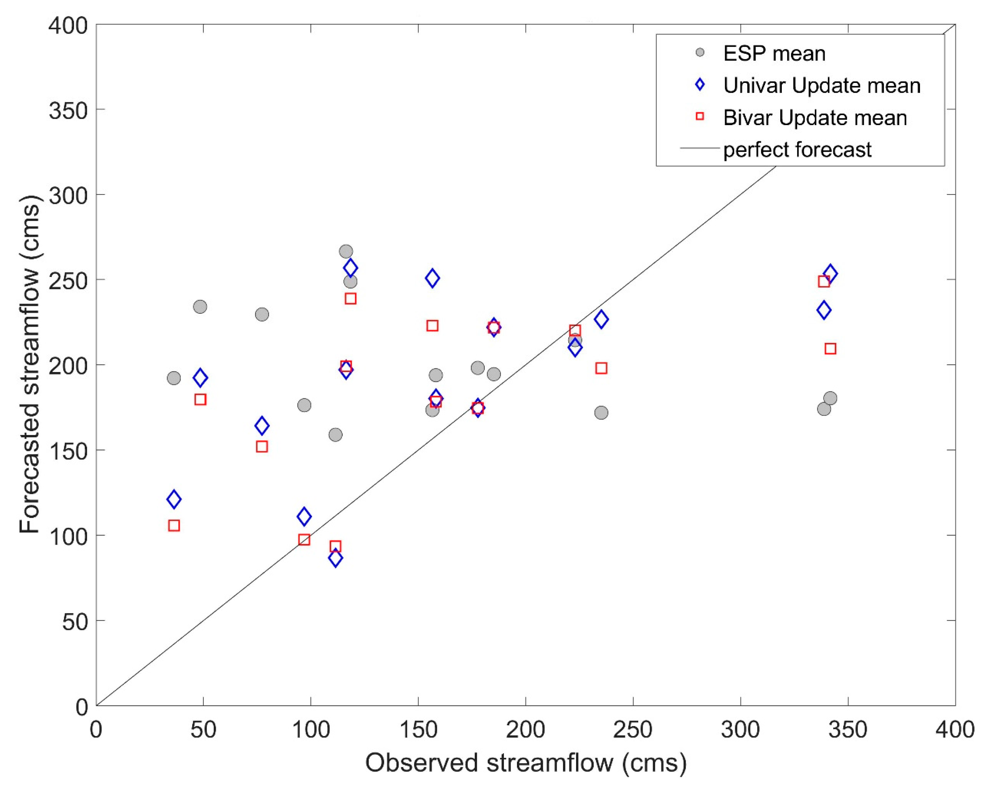
Figure 11 shows a scatter plot that demonstrates a case in which Bivar_update model outperforms Univar_update model in terms of forecast accuracy. It displays observed monthly streamflow of Soyanggang dam watershed (#1 on Table 1) in August on the horizontal axis and corresponding forecasted monthly streamflow on the vertical axis under the most accurate PPF and PTF case (P100 & T100). Results from a single watershed are visualized for easier interpretation and general discussion. In Figure 11 it is found that the both models are able to reduce forecasting errors when the accurate climate forecast information is given. R2 value of ESP mean, Univar_update, and Bivar_update models were 0.14, 0.35, and 0.44, respectively. When it comes to a total of 35 watersheds, the median values of R2 of ESP mean, Univar_update, and Bivar_update models were 0.06 (0.00, 0.21), 0.40 (0.16, 0.75), and 0.43 (0.21, 0.74), respectively (lower and upper limits of confidence interval are shown in parenthesis). Although the plots of all the watersheds for all of twelve months cannot be presented here, Bivar_update model overall was able to further improve the streamflow predictability of Univar_update model across varying PPF and PTF performance as shown in Figure 5, Figure 6, Figure 7, Figure 8, Figure 9 and Figure 10.

5. Discussion and Conclusions

The present study developed a simple yet efficient approach incorporating probabilistic forecast information to the ensemble streamflow forecasts obtained by the ESP. The proposed method, the Bivar_update model, utilizes both precipitation and temperature forecasts to update individual weights on each streamflow prediction scenario based on the Bayesian updating scheme with discrete priors. The performance of the Bivar_update model was evaluated through its comparison with the Univar_update model that reflected only precipitation forecasts. Overall, the Bivar_update outperformed the Univar_update in terms of both deterministic and categorical forecast skill. The superiority of the Bivar_update model was remarkable across all the cases of synthetic probabilistic forecasts series especially under dry conditions.
Although the current study proposed a simple and straightforward method to incorporate bivariate climate forecast information on the probabilities of ensemble forecasts from the ESP, there is still room for improvement. First, the co-dependency between precipitation and temperature is considered for neither a synthetic probabilistic forecast generator nor the Bivar_update model for the sake of easy applicability. Seo et al. [27] discussed that co-dependency between precipitation and temperature needed to be considered in hydrologic simulations. Nonetheless, co-dependency between precipitation and temperature is significant only for several months (e.g., winter and summer in South Korea), and it is not homogenous at a spatial level depending on climate regimes. Co-dependency between precipitation and temperature forecasts was not considered in this study for easier application. Therefore, incorporating the co-dependency between precipitation and temperature forecast could be a future extension of the proposed methodology. In addition, a reduction in a variance of ensemble forecasts would be worth for operational forecast since decision makers are reluctant to consider a huge variance in ensemble forecasts. Increasing precision, that is, cutting off variability of ensemble forecasts, also could be a potential extension of this study. This kind of uncertainty quantification in ensemble forecasts is closely relevant to flood forecasting system and mitigation of natural hazard. For this purpose, temporal and spatial scales of the forecasting system should be finer and fully distributed hydrological models would be required.
Furthermore, Croley–Wilks approach which is adopted in the proposed methodology can be replaced to the PDF-ratio method which can complement the limitations of the Croley–Wilks approach. The readers refer to Stedinger and Kim [35] for details about the comparison between the Croley–Wilks and the PDF-ratio approaches. Although the authors used the Croley–Wilks approach, PDF-ratio approach can also be applied if the joint PDF of precipitation and temperature forecasts is obtained. Since the ensemble of the precipitation and temperature forecasts is not yet provided from KMA (in other words, only tercile probabilities of the precipitation and temperature forecasts are provided), the joint PDF of the both forecasts could not be estimated.
The primary implications from the analyses are two-fold. First, incorporating temperature forecast information should not be overlooked. The current study demonstrated that reliable PTFs have the capability of enhancing the accuracy of ensemble forecasts from the ESP. Moreover, there is a general consensus that uncertainty is greater in precipitation forecast than temperature forecast. For instance, when it comes to the probabilistic climate forecasts, which are reported by the KMA of South Korea, the general predictability of PTFs is greater than that of PPFs. Nonetheless, little effort has been contributed to enhance streamflow-forecasting skill by utilizing the given PTF information. In this regard, employing the proposed Bivar_update model would be a step towards improvement in the streamflow forecasting system. Since the Bivar_update model is theoretically straightforward and easy to implement, it would not be difficult to practically implement it on site.
In addition, this study discusses that incorporating temperature forecast information can increase streamflow forecasting skill when the role of temperature in streamflow forecast is significant, such as snow-dominated and evapotranspiration-dominated regions. It is obvious that snow-melting and evapotranspiration are strongly dependent on temperature, therefore this study was motivated since there have been a few efforts on a systematic analysis of the role of temperature forecast in increasing streamflow predictability. As discussed above, the superiority of the Bivar_update model is more prominent under dry conditions: When the role of temperature increases. Since the runoff sensitivity to temperature increases under dry conditions, the prediction skill for streamflow can be efficiently improved by incorporating reliable temperature forecast information. Therefore, the Bivar_update model successfully enhanced both deterministic and probabilistic streamflow forecast skill, thereby outperforming the Univar_update that only considers precipitation forecast information. Therefore, its implications can be extended to low-flow prediction. Since the Bivar_update model uses both precipitation and temperature information, it is able to compensate low predictability especially under below normal condition in which streamflow’s dependency on temperature increases. Hence, enhanced skill in forecasting temperature can complement the lack of precipitation forecast skill in where temperature plays an important role in streamflow forecast. It should be noted that the advantage of temperature forecast in streamflow would be negligible when it comes to regions and seasons the temperature do not affect the streamflow forecast. Additionally, the performance of the Bivar_update model is evaluated by synthetic climate forecast information, and the improvement obtained by the Bivar_update model is still low. Hence, the more in-depth case studies across a variety of climate regimes should be followed.
Lastly, evapotranspiration, which is strongly relying on temperature, is also dependent on types of soil and the slope of the relief along with local microclimates. This study was not able to reflect these kinds of details in climatic geomorphology since a lumped hydrological model was adopted in this study. Although there are several parameters that conceptualized the hydro-geomorphological characteristics in the model, it cannot reflect heterogeneity of the characteristics. To address the effect of heterogeneity of the microclimates and geomorphology on streamflow predictability, the Bivar_update model can be implemented to fully distribute hydrological models for a following study.

Author Contributions

Conceptualization, J.H.S. and S.B.S.; methodology, J.H.S. and S.B.S.; software, Y.R.; validation, J.H.S. and S.B.S.; formal analysis, Y.R., J.H.S. and S.B.S.; investigation, S.B.S.; resources, J.H.S. and Y.R.; data curation, J.H.S.; writing—original draft preparation, J.H.S.; writing—review and editing, Y.R. and S.B.S.; visualization, J.H.S.; supervision, S.B.S.; project administration, S.B.S.; funding acquisition, S.B.S. All authors have read and agreed to the published version of the manuscript.

Funding

This research was funded by the Young Researchers program [NRF-2017R1A6A3A11031800] funded by the National Research Foundation of Korea.

Acknowledgments

This work was supported by the Young Researchers program [NRF-2017R1A6A3A11031800] funded by the National Research Foundation of Korea. The authors also thank for University of Seoul for their support. All data necessary to reproduce the results of this study are available from the authors upon request.

Conflicts of Interest

The authors declare no conflict of interest.

Appendix A. Utilizing Univariate Climate Forecast Information

Given that the probabilistic precipitation forecast is provided as a form of three interval probabilities, the prior probabilities on each historical climate series, 1 / N , are simply updated to p x , b / N b , p x , n / N n , and p x , a / N a for below-normal, normal, and above-normal respectively. N b ,   N n , and N a refer to the number of historical precipitation scenarios that belong to below-normal, normal, and above-normal ranges respectively, i.e., N b + N n + N a = N . The Croley-Wilks probabilities p x , b / N b , p x , n / N n , and p x , a / N a are simple solutions that match the required probabilities for below-normal (bn), normal (n), and above-normal (an) events (Kim and Stedinger, 2010). Based on the adjusted probabilities of the climate scenarios in each interval, the ensemble mean of streamflow forecast, μ q , is calculated as below,
μ q = μ q b + μ q n + μ q   a ,
where μ q b = ( p x , b / N b ) q i ( only   when   x i x b ) , μ q n = ( p x , n / N n ) q i ( only   when   x b < x i x a ) , μ q a = ( p x , a / N a ) q i ( only   when   x a < x i ) , and q i is simulated streamflow driven by ith climate scenario (i.e., q i is a function of x i and y i ).
The underlying assumption behind this calculation is that the probability assigned to a climate scenario is applied to the matching streamflow scenario simulated by the climate scenario. Note that without climate forecast information, μ q is calculated as a value of the simple mean of q i , i.e., μ q = 1 N q i .

Appendix B. Utilizing Bivariate Climate Forecast Information
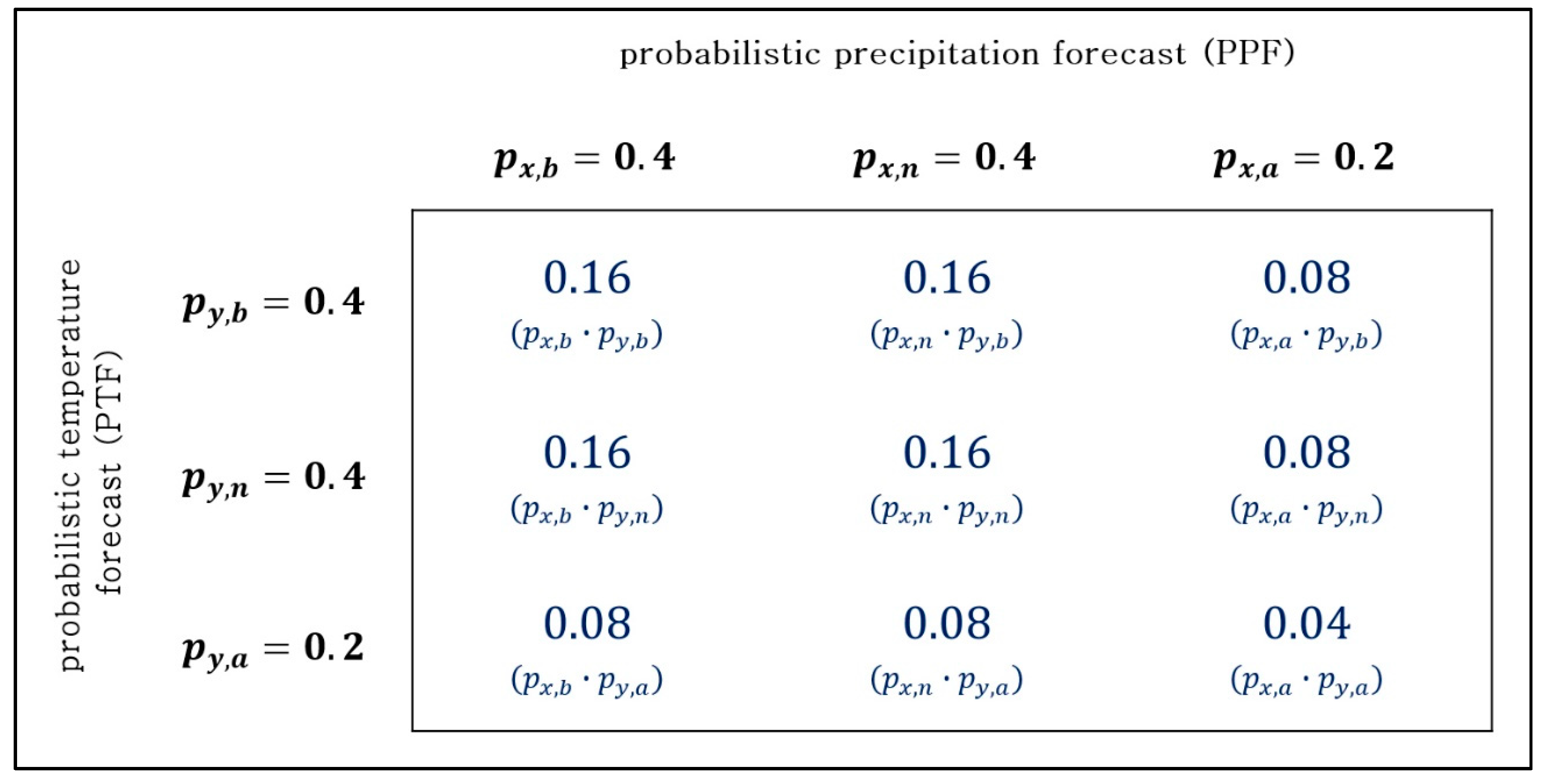
Figure A1. Demonstration of prior joint PMF estimation.
Sustainability 12 02905 g0a1
For instance, if the marginal PMF for both the P 1 and P 2 are given as P P 1 ( p 1 = BN ) = p 1 , b = 0.4 , P P 1 ( p 1 = N ) = p 1 , n = 0.4 , P P 1 ( p 1 = AN ) = p 1 , a = 0.2 , P P 2 ( p 2 = BN ) = p 2 , b = 0.4 , P P 2 ( p 2 = N ) = p 2 , n = 0.4 , and P P 2 ( p 2 = AN ) = p 2 , a = 0.2 , all of the individual joint probability are simply calculated as shown in Figure A1.
Figure A2. Demonstration of likelihood function estimation.
Sustainability 12 02905 g0a2

Appendix C. Contingency Table for the 3 × 3 Categorical Forecast Verification

Figure A3. Contingency table for the 3 × 3 categorical forecast verification.
Sustainability 12 02905 g0a3

Appendix D. Realization of Synthetic Probabilistic Forecasts

The two steps used for generating the synthetic probabilistic forecasts are described below.
1)
setting up a group of historic forecasts: Obtain historic forecasts that were issued up to date and categorize them into the three intervals (below-normal, normal, and above-normal). Historical forecast samples are presented in Table A1
2)
random sampling: Extract samples randomly from the group of historic forecast samples in order to allow them to have targeting the POD value. For instance, if an observed climate scenario belongs to the below-normal interval and the given value of the target POD is 0.5, half of the forecasts are randomly sampled among the historical forecasts that belong to the below-normal category, while the other half of forecasts are randomly sampled among the historical forecasts that do not belong to the below-normal category. Figure A4 illustrates an example of the synthetic probabilistic forecast generation. First, randomly select a single forecast for each category among all the historic samples. A final forecast must be selected among these three candidates based on given weights (i.e., extraction probability) that vary corresponding to the value of the target POD. Thus, extraction probability is the given weights for the three different categories (below-normal, normal, and above-normal) in order to synthetically generate probabilistic climate forecast series. This must be repeated till the end of time step and separately generated for each province. The PPF and the PTF series are generated separately, since it is assumed that PPFs and PTFs are independent. Note that the synthetic forecast generated in the Figure A4 is just an example.
Eight cases of synthetic probabilistic forecast (POD value ranging from 0.3 to 1.0 and increasing by 0.1) were generated for each PPF and PTF, so the total number of synthetic probabilistic forecast pairs became 64 (i.e., 8 × 8 = 64). Hundred different synthetic probabilistic forecast series were generated for each of the 64 combinations.
Table A1. Historical forecast samples that were issued up to date. A forecast sample which below-normal probability is equal or greater than 0.5 becomes a member of the below-normal forecast. On the other hand, a forecast sample which above-normal probability is equal or greater than 0.5 becomes a member of the above-normal forecast. If a forecast does not belong to neither below nor above-normal, it becomes a member of normal forecast. The number of samples for both below and above-normal is 9 whereas the number of samples for normal is 40.
Below-NormalNormalAbove-Normal
p b p n p a p b p n p a p b p n p a
0.500.400.100.250.300.450.100.400.50
0.500.350.150.300.300.400.150.350.50
0.500.300.200.400.300.300.200.300.50
0.550.350.100.450.300.250.100.350.55
0.550.300.15:::0.150.300.55
0.600.300.100.250.600.150.100.300.60
0.600.250.150.300.600.100.150.250.60
0.650.250.100.200.650.150.100.250.65
0.700.200.100.150.650.200.100.200.70
Figure A4. An example of the synthetic probabilistic forecasts generation.
Sustainability 12 02905 g0a4

References

  1. Ding, W.; Zhang, C.; Peng, Y.; Zeng, R.; Zhou, H.; Cai, X. An analytical framework for flood water conservation considering forecast uncertainty and acceptable risk. Water Resour. Res. 2015, 51, 4702–4726. [Google Scholar] [CrossRef]
  2. Pappenberger, F.; Cloke, H.L.; Parker, D.J.; Wetterhall, F.; Richardson, D.S.; Thielen, J. The monetary benefit of early flood warnings in Europe. Environ. Sci. Policy 2015, 51, 278–291. [Google Scholar] [CrossRef]
  3. Seo, S.B.; Kim, Y.-O.; Kim, Y.; Eum, H.-I. Selecting climate change scenarios for regional hydrologic impact studies based on climate extremes indices. Clim. Dyn. 2019, 52, 1595–1611. [Google Scholar] [CrossRef]
  4. Steinemann, A.C. Using climate forecasts for drought management. J. Appl. Meteorol. Climatol. 2006, 45, 1353–1361. [Google Scholar] [CrossRef]
  5. Eum, H.I.; Kim, Y.O.; Palmer, R.N. Optimal drought management using sampling stochastic dynamic programming with a hedging rule. J. Water Resour. Plan. Manag. 2011, 137, 113–122. [Google Scholar] [CrossRef]
  6. Eum, H.-I.; Kim, Y.-O. The value of updating ensemble streamflow prediction in reservoir operations. Hydrol. Process. 2010, 24, 2888–2899. [Google Scholar] [CrossRef]
  7. Georgakakos, A.P.; Yao, H.; Kistenmacher, M.; Georgakakos, K.P.; Graham, N.E.; Cheng, F.-Y.; Spencer, C.; Shamir, E. Value of adaptive water resources management in Northern California under climatic variability and change: Reservoir management. J. Hydrol. 2012, 412–413, 34–46. [Google Scholar] [CrossRef]
  8. Day, G.N. Extended streamflow forecasting using NWSRFS. J. Water Resour. Plan. Manag. 1985, 111, 157–170. [Google Scholar] [CrossRef]
  9. Schaake, J.; Larson, L. Ensemble Streamflow Prediction (ESP): Progress and Research Needs. In Special Symposium on Hydrology; American Meteorological Society: Boston, MA, USA, 1998. [Google Scholar]
  10. Kim, Y.-O.; Jeong, D.-I.; Kim, H.-S. Improving water supply outlook in Korea with ensemble streamflow prediction. Water Int. 2001, 26, 563–568. [Google Scholar] [CrossRef]
  11. Franz, K.J.; Hartmann, H.C.; Sorooshian, S.; Bales, R. Verification of national weather service ensemble streamflow predictions for water supply forecasting in the Colorado River basin. J. Hydrometeorol. 2003, 4, 1105–1118. [Google Scholar] [CrossRef] [Green Version]
  12. Jeong, D.-I.; Kim, Y.-O. Rainfall-runoff models using artificial neural networks for ensemble streamflow prediction. Hydrol. Process. 2005, 19, 3819–3835. [Google Scholar] [CrossRef]
  13. Gobena, A.K.; Gan, T.Y. Incorporation of seasonal climate forecasts in the ensemble streamflow prediction system. J. Hydrol. 2010, 385, 336–352. [Google Scholar] [CrossRef]
  14. Najafi, M.R.; Moradkhani, H.; Piechota, T.C. Ensemble streamflow prediction: Climate signal weighting methods vs. climate forecast system reanalysis. J. Hydrol. 2012, 442–443, 105–116. [Google Scholar] [CrossRef]
  15. Wood, A.; Sankarasubramanian, A.; Mendoza, P. Seasonal Ensemble Forecast Post-processing. In Handbook of Hydrometeorological Ensemble Forecasting; Duan, Q., Pappenberger, F., Wood, A., Cloke, H.L., Schaake, J.C., Eds.; Springer: Berlin/Heidelberg, Germany, 2019; pp. 819–845. ISBN 978-3-642-39925-1. [Google Scholar]
  16. Kelman, J.; Stedinger, J.R.; Cooper, L.A.; Hsu, E.; Yuan, S.-Q. Sampling stochastic dynamic programming applied to reservoir operation. Water Resour. Res. 1990, 26, 447–454. [Google Scholar] [CrossRef]
  17. Faber, B.A.; Stedinger, J.R. Reservoir optimization using sampling SDP with ensemble streamflow prediction (ESP) forecasts. J. Hydrol. 2001, 249, 113–133. [Google Scholar] [CrossRef]
  18. Krzysztofowicz, R. Integrator of uncertainties for probabilistic river stage forecasting: Precipitation-dependent model. J. Hydrol. 2001, 249, 69–85. [Google Scholar] [CrossRef]
  19. Herr, H.D.; Krzysztofowicz, R. Bayesian ensemble forecast of river stages and ensemble size requirements. J. Hydrol. 2010, 387, 151–164. [Google Scholar] [CrossRef] [Green Version]
  20. Demargne, J.; Wu, L.; Regonda, S.K.; Brown, J.D.; Lee, H.; He, M.; Seo, D.-J.; Hartman, R.; Herr, H.D.; Fresch, M.; et al. The science of NOAA’s operational hydrologic ensemble forecast service. Bull. Am. Meteorol. Soc. 2013, 95, 79–98. [Google Scholar] [CrossRef]
  21. Beckers, J.V.L.; Weerts, A.H.; Tijdeman, E.; Welles, E. ENSO-conditioned weather resampling method for seasonal ensemble streamflow prediction. Hydrol. Earth Syst. Sci. 2016, 20, 3277–3287. [Google Scholar] [CrossRef] [Green Version]
  22. Ye, A.; Deng, X.; Ma, F.; Duan, Q.; Zhou, Z.; Du, C. Integrating weather and climate predictions for seamless hydrologic ensemble forecasting: A case study in the Yalong River basin. J. Hydrol. 2017, 547, 196–207. [Google Scholar] [CrossRef]
  23. Cuo, L.; Pagano, T.C.; Wang, Q.J. A review of quantitative precipitation forecasts and their use in short- to medium-range streamflow forecasting. J. Hydrometeorol. 2011, 12, 713–728. [Google Scholar] [CrossRef]
  24. Bennett, J.C.; Wang, Q.J.; Li, M.; Robertson, D.E.; Schepen, A. Reliable long-range ensemble streamflow forecasts: Combining calibrated climate forecasts with a conceptual runoff model and a staged error model. Water Resour. Res. 2016, 52, 8238–8259. [Google Scholar] [CrossRef]
  25. Barnett, T.P.; Adam, J.C.; Lettenmaier, D.P. Potential impacts of a warming climate on water availability in snow-dominated regions. Nature 2005, 438, 303–309. [Google Scholar] [CrossRef] [PubMed]
  26. Shukla, S.; Safeeq, M.; AghaKouchak, A.; Guan, K.; Funk, C. Temperature impacts on the water year 2014 drought in California. Geophys. Res. Lett. 2015, 42, 4384–4393. [Google Scholar] [CrossRef] [Green Version]
  27. Seo, S.B.; Das Bhowmik, R.; Sankarasubramanian, A.; Mahinthakumar, G.; Kumar, M. The role of cross-correlation between precipitation and temperature in basin-scale simulations of hydrologic variables. J. Hydrol. 2019, 570, 304–314. [Google Scholar] [CrossRef]
  28. Scheuerer, M.; Hamill, T.M.; Whitin, B.; He, M.; Henkel, A. A method for preferential selection of dates in the Schaake shuffle approach to constructing spatiotemporal forecast fields of temperature and precipitation. Water Resour. Res. 2017, 53, 3029–3046. [Google Scholar] [CrossRef]
  29. Chen, J.; Li, C.; Brissette, F.P.; Chen, H.; Wang, M.; Essou, G.R.C. Impacts of correcting the inter-variable correlation of climate model outputs on hydrological modeling. J. Hydrol. 2018, 560, 326–341. [Google Scholar] [CrossRef]
  30. Bhowmik, R.D.; Sankarasubramanian, A.; Sinha, T.; Patskoski, J.; Mahinthakumar, G.; Kunkel, K.E. Multivariate downscaling approach preserving cross correlations across climate variables for projecting hydrologic fluxes. J. Hydrometeorol. 2017, 18, 2187–2205. [Google Scholar] [CrossRef]
  31. Seo, S.B.; Kim, Y.-O.; Kang, S.-U.; Chun, G.I. Improvement in long-range streamflow forecasting accuracy using the Bayes’ theorem. Hydrol. Res. 2019, 50, 616–632. [Google Scholar] [CrossRef]
  32. Croley, T.E. Weighted-climate parametric hydrologic forecasting. J. Hydrol. Eng. 2003, 8, 171–180. [Google Scholar] [CrossRef]
  33. Croley, T.E. Using Meteorology Probability Forecasts in Operational Hydrology; American Society of Civil Engineers: Reston, VA, USA, 2000; ISBN 978-0-7844-0459-1. [Google Scholar]
  34. Wilks, D.S. Realizations of daily weather in forecast seasonal climate. J. Hydrometeorol. 2002, 3, 195–207. [Google Scholar] [CrossRef]
  35. Stedinger, J.R.; Kim, Y.-O. Probabilities for ensemble forecasts reflecting climate information. J. Hydrol. 2010, 391, 9–23. [Google Scholar] [CrossRef]
  36. Kim, H.S.; Jeon, K.I.; Kang, S.U.; Nam, W.S. The study on the weighting method of ESP based on probabilistic long-term forecast. Proc. KSCE Conv. 2016, 91–92. [Google Scholar]
  37. Wilks, D.S. Statistical Methods in the Atmospheric Sciences, 3rd ed.; Academic Press: San Diego, CA, USA, 2011; Volume 100. [Google Scholar]
  38. Allen, R.G.; Pereira, L.S.; Raes, D.; Smith, M. FAO Irrigation and Drainage Paper; FAO UN: Rome, Italy, 1998; p. 326. [Google Scholar]
  39. Brassel, K.E.; Reif, D. A procedure to generate thiessen polygons. Geogr. Anal. 1979, 11, 289–303. [Google Scholar] [CrossRef]
  40. Jeong, J.-H.; Lee, H.; Yoo, J.H.; Kwon, M.; Yeh, S.-W.; Kug, J.-S.; Lee, J.-Y.; Kim, B.-M.; Son, S.-W.; Min, S.-K.; et al. The status and prospect of seasonal climate prediction of climate over Korea and East Asia: A review. Asia-Pac. J. Atmos. Sci. 2017, 53, 149–173. [Google Scholar] [CrossRef]
  41. Sugawara, M. Tank model. In Computer Models of Watershed Hydrology; Singh, B.P., Ed.; Water Resources Pubns: Highlands Ranch, CO, USA, 1995; ISBN 978-1-887201-74-2. [Google Scholar]
  42. McCabe, G.J.; Markstrom, S.L. A Monthly Water-Balance Model Driven by a Graphical User Interface; Open-File Report; Geological Survey (U.S.): Reston, VA, USA, 2007.
  43. McCabe, G.J.; Wolock, D.M. General-Circulation-Model simulations of future snowpack in the Western United states. JAWRA J. Am. Water Resour. Assoc. 1999, 35, 1473–1484. [Google Scholar] [CrossRef]
  44. Duan, Q.; Sorooshian, S.; Gupta, V. Effective and efficient global optimization for conceptual rainfall-runoff models. Water Resour. Res. 1992, 28, 1015–1031. [Google Scholar] [CrossRef]
  45. Seo, S.B.; Kim, Y.-O. Impact of spatial aggregation level of climate indicators on a national-level selection for representative climate change scenarios. Sustainability 2018, 10, 2409. [Google Scholar] [CrossRef] [Green Version]
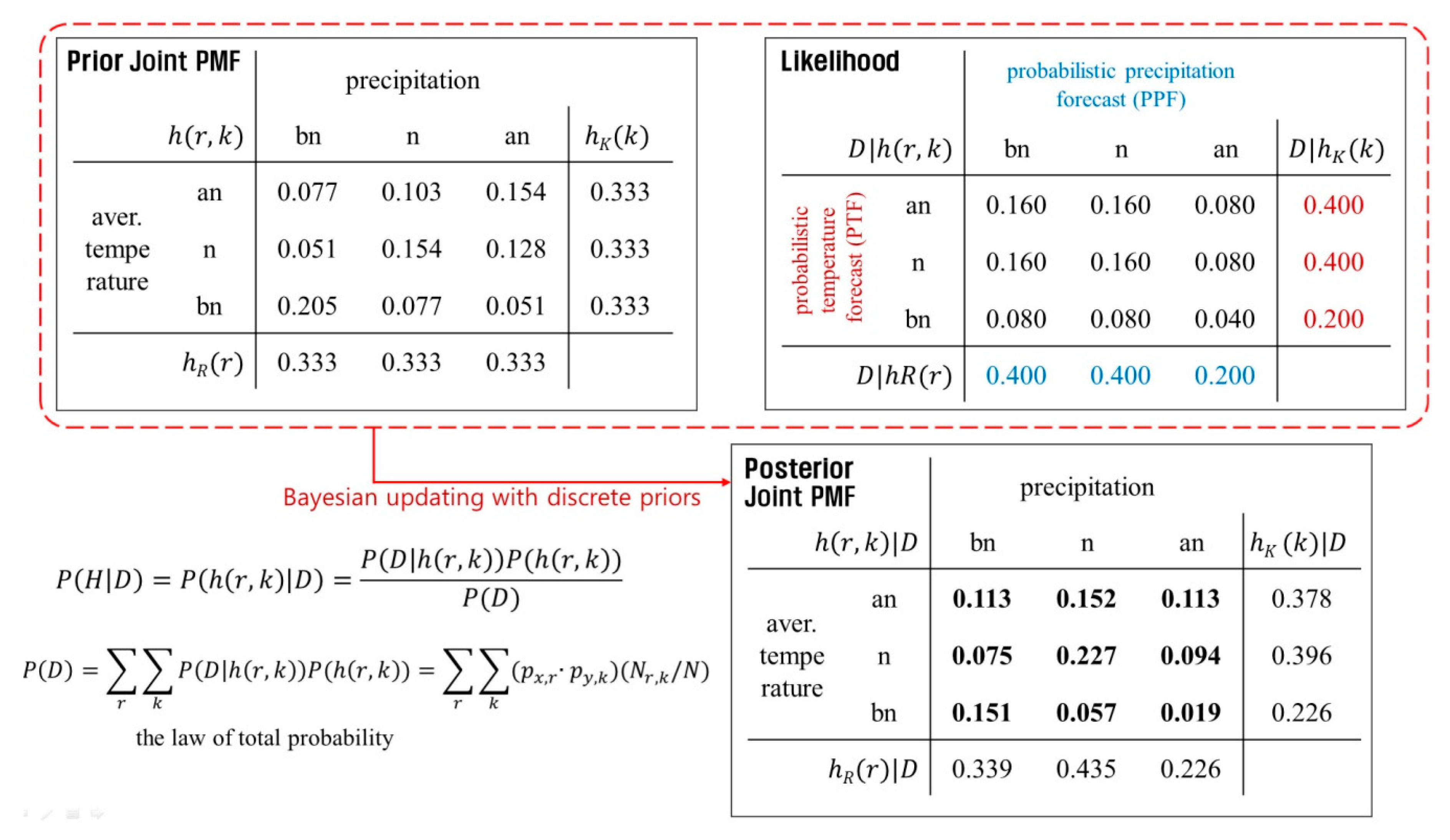
Figure 1. Demonstration of an example calculation of a posterior joint probability mass function (PMF) with discrete priors; bn: below-normal, n: normal, an: above-normal.
Sustainability 12 02905 g001
Figure 2. Thirty-five dam basins and sixty ASOS (Automated Synoptic Observing System) weather stations used in this study.
Sustainability 12 02905 g002
Figure 3. An example of a three-month-ahead probability forecast for precipitation and average temperature issued by Korea Meteorological Administration.
Sustainability 12 02905 g003
Figure 4. Overall evaluation framework for this study; PPF: probabilistic precipitation forecast, PTF: probabilistic temperature forecast, POD: probability of detection.
Sustainability 12 02905 g004
Figure 5. NRMSE results for the three forecasting models—ESP, Univar_update, and Bivar_update. Left column figures present NRMSE results calculated from all the forecasts. The right column figures present NRMSE results calculated from only forecasts when the observed values are under below-normal conditions. (a) 30% POD for PPF and 30% POD for PTF (P30–T30), (b) 50% POD for PPF and 50% POD for PTF (P50–T50), (c) 70% POD for PPF and 70% POD for PTF (P70–T70), (d) 100% POD for PPF and 100% POD for PTF (P100–T100).
Sustainability 12 02905 g005
Figure 6. Comparison of errors in streamflow predictions between the three forecasting models—(a) Differences in NRMSE values between the Univar_update and the ESP (negative value represents outperformance by the Univar_update). (b) Differences in NRMSE values between the Bivar_update and the Univar_update (negative value represents outperformance by the Bivar_update).
Sustainability 12 02905 g006
Figure 7. Comparison of errors in streamflow predictions between the three forecasting models under below-normal conditions. (a) Differences in NRMSE values between the Univar_update and the ESP (negative value represents outperformance by the Univar_update). (b) Differences in NRMSE values between the Bivar_update and the Univar_update (negative value represents outperformance by the Bivar_update).
Sustainability 12 02905 g007
Figure 8. The POD results for the three forecasting models—ESP, Univar_update, and Bivar_update. The left column figures present the POD results calculated from all the forecasts. The right column figures present the POD results calculated from only forecasts when observed values are under a below-normal condition. (a) 30% POD for PPF and 30% POD for PTF (P30–T30), (b) 50% POD for PPF and 50% POD for PTF (P50–T50), (c) 70% POD for PPF and 70% POD for PTF (P70–T70), (d) 100% POD for PPF and 100% POD for PTF (P100–T100).
Sustainability 12 02905 g008
Figure 9. Comparison of categorical streamflow prediction skills between the three forecasting models: (a) Differences in the POD values between the Univar_update and the ESP (positive value represents outperformance by the Univar_update). (b) Differences in the POD values between the Bivar_update and the Univar_update (positive value represents outperformance by the Bivar_update).
Sustainability 12 02905 g009
Figure 10. Comparison of categorical streamflow prediction skills between the three forecasting models under below-normal conditions. (a) Differences in the POD values between the Univar_update and the ESP (positive value represents outperformance by the Univar_update). (b) Differences in the POD values between the Bivar_update and the Univar_update (positive value represents outperformance by the Bivar_update).
Sustainability 12 02905 g010
Figure 11. A scatter plot that displays observed monthly streamflow of Soyanggang dam watershed (#1 in Table 1) in August on the horizontal axis and corresponding forecasted monthly streamflow on the vertical axis under the most accurate PPF and PTF case (P100 & T100). Grey circles, blue diamonds, red squares are ensemble mean forecast of ESP, Univar_update, Bivar_update model, respectively. (unit: cms, cubic meters per second).
Sustainability 12 02905 g011
Table 1. A list of the 35 dams used in this study.
No.NameDrainage Areas (km2)Reservoir Capacity (Million Cubic Meters)
1Andong1584 1248
2Angye7 18
3Bohyunsan33 22
4Boryeong164 117
5Buan59 50
6Chungju6648 2750
7Daeam77 13
8Daecheong3204 1490
9Daegok58 36
10Dalbang29 9
11Gampo4 3
12Gucheon13 10
13Gunwi88 49
14Gwangdong125 13
15Hapcheon925 790
16Heongseong209 87
17Imha1361 595
18Jangheung193 191
19Juam1010 457
20Juam regulator135 250
21Kimcheonbuhang82 54
22Miryang95 74
23Namgang2285 309
24Pyeongnim20 10
25Sayeon67 30
26Seomjin763 466
27Seonam1 2
28Seongdeok41 28
29Soyanggang2703 2900
30Sueo49 31
31Woonmoon301 160
32Yeoncho12 5
33Yeongcheon235 103
34Yeongju500 181
35Yongdam930 815