Abstract
Despite the fact that fine particulate matter (PM2.5) causes serious health issues, few studies have investigated the level and annual rate of PM2.5 change across a large number of countries. For a better understanding of the global trend of PM2.5, this study classified 190 countries into groups showing different trends of PM2.5 change during the 2000–2014 period by estimating the progress ratio (PR) from the experience curve (EC), with PM2.5 exposure (PME)–the population-weighted average annual concentration of PM2.5 to which a person is exposed—as the dependent variable and the cumulative energy consumption as the independent variable. The results showed a wide variation of PRs across countries: While the average PR for 190 countries was 96.5%, indicating only a moderate decreasing PME trend of 3.5% for each doubling of the cumulative energy consumption, a majority of 118 countries experienced a decreasing trend of PME with an average PR of 88.1%, and the remaining 72 countries displayed an increasing trend with an average PR of 110.4%. When two different types of EC, classical and kinked, were applied, the chances of possible improvement in the future PME could be suggested in the descending order as follows: (1) the 60 countries with an increasing classical slope; (2) the 12 countries with an increasing kinked slope; (3) the 75 countries with a decreasing classical slope; and (4) the 43 countries with a decreasing kinked slope. The reason is that both increasing classical and kinked slopes are more likely to be replaced by decreasing kinked slopes, while decreasing classical and kinked slopes are less likely to change in the future. Population size seems to play a role: A majority of 52%, or 38 out of the 72 countries with an increasing slope, had a population size of bigger than 10 million inhabitants. Many of these countries came from SSA, EAP, and LAC regions. By identifying different patterns of past trends based on the analysis of PME for individual countries, this study suggests a possible change of the future slope for different groups of countries.
1. Introduction
The cost of the health impact of ambient air pollution was about $1.7 trillion in OECD (Organisation for Economic Co-operation and Development) countries and $1.4 trillion in China alone [1]. Among different pollutants, fine particulate matter (PM2.5), an atmospheric particle of 2.5 microns or less in diameter, has drawn significant attention because it is small enough to lodge into human lungs and is believed to cause serious damages, such as high mortality [2], premature deaths [3], and heart and lung diseases [4]. To cope with high levels of PM2.5, the World Health Organization (WHO) has established an annual mean value of 10 micrograms per cubic meter (μg/m3) as the recommended guideline for long-term exposure to PM2.5 [5]. Recognizing that it will take some time for many countries to comply with this guideline, the WHO has provided three interim targets of 15 μg/m3, 25 μg/m3, and 35 μg/m3 for PM2.5. Legally-enforced standards for the annual mean level of PM2.5 vary across countries ranging from Australia’s 8 μg/m3 [6], the United States’ 12 μg/m3 [7], to the European Union’s 25 μg/m3 [8].
Due to serious health implications, there have been numerous studies dealing with PM2.5 emission and its impact on mortality and life expectancy in multiple countries [9,10,11,12,13]. Further, because of the very high PM2.5 concentration in China, an equally large number of studies focusing on spatio-temporal variations and socioeconomic drivers of PM2.5 emissions in China have appeared in recent years [14,15,16,17]. However, there are only a few studies dealing with the analysis of changing historical trends of PM2.5 for multiple countries.
According to a recent convergence study for 212 countries, the average PM2.5 exposure (PME), measuring the average annual concentration of PM2.5 to which a person is exposed on a typical day, demonstrated a wide variation over time [18]. While the compounded annual growth rate (CAGR) for PME for a total of 212 countries was estimated to be −0.21% during the 2000–2014 period, the average PME was 7.60 μg/m3 in 2000, peaked at 8.60 μg/m3 in 2007, and then decreased to 7.38 μg/m3 in 2014. Regional differences were significant as well. For example, the average PME of eight countries in the South Asia region was 12.91 μg/m3 in 2000 and increased to 19.55 μg/m3 in 2014, recording a CAGR of 3.01%. In contrast, the average PME of 59 countries in the Europe and Central Asia and North America region was 11.31 μg/m3 in 2000 and declined to 8.82 μg/m3 in 2014, registering a CAGR of −1.76%.
Another recent paper [19] shows that countries individually also displayed widely varying annual rates of change in their PME during the 2000–2014 period. For example, as illustrated in Table 1, ten countries with the highest PME in 2014 displayed widely varying CAGRs, ranging from 4.48% in Bangladesh to −2.50% in Hungary during the 2000–2014 period. In contrast, all ten countries with the lowest PME experienced negative CAGRs, ranging from −10.19% in the Marshall Islands to −1.58% in Kiribati. These examples show that the rate of change in PME over time varies greatly across individual countries: Some countries exhibited continuously increasing/decreasing rates, while other countries experienced variable increasing/decreasing rates.

Table 1.
Annual growth or reduction rates of the top ten and bottom ten countries in particulate matter exposure (PME).
The main objective of this research is to estimate the historical trend of PME with the slope from an experience curve (EC) for each of 190 countries during the 2000–2014 period and classify them into groups showing different trends of PME change over time. Unlike the two convergence analysis studies mentioned above [18,19] that only documented the changes of PME over time and comparing them across multiple groups of countries, this study employs EC which allows us to show the historical trend of PME in connection with the cumulative energy consumption.
Among such key socioeconomic factors influencing the level of PME as population, income, urbanization, industrialization, and energy consumption [20,21,22,23], the cumulative primary energy consumption was selected as an independent variable to drive EC. According to the 2018 Special Report on Energy and Air Pollution by the International Energy Agency [24], some 85% of global emissions of particulate matter generated by human activity is derived from energy production and use, mainly the combustion of fossil fuels and biomass in the building, industry, and transport sectors. The impact of industrial and non-industrial combustion and vehicle traffic on the level of particulate matter is documented at the city level as well [25]. Fossil fuels continue to dominate the global energy mix in that the overall share of oil, coal, and natural gas accounted for the same 81% of the total energy used during the last 25 years. In another recent study of 141 countries on PM2.5 concentrations determined that the most important impact factor in relation to PM2.5 concentrations was energy consumption structure for the lower-middle and low-income groups of countries [26]. Much of the scholarship agrees that fossil fuel affected PM2.5 concentrations [27,28,29,30,31,32,33].
In addition, many other studies have indicated a close relationship between fossil fuels consumption to other influencing socioeconomic factors, such as urbanization, economic development, and industrialization for high PM2.5 [30,34,35,36,37,38,39,40,41]. On the other hand, energy consumption efficiency, energy intensity, and per capita energy consumption differ among countries [42]. Therefore, the impact of energy consumption on the level of PM2.5 should vary across countries. In summary, the use of energy consumption as the key influencing factor will enable this research to focus on the impact of human activity on PME. Thus, the analysis of natural influencing factors of climate and ecosystem elements such as wind, temperature precipitation, topography, land use, and others is beyond the scope of this research.
The slope of EC, known as the progress ratio (PR) expressed in percentage, is informative. For example: A declining slope of 80% PR means that each doubling of the independent variable, the cumulative energy consumption in this study, has generated a 20% reduction of PME, whereas an increasing slope of 120% PR means that each doubling of the cumulative energy consumption has produced a 20% increase of PME. In addition, two types of EC—classical and kinked—provide us with an opportunity to identify varying rates of change that can take place during the period of analysis. While this type of analysis alone is not capable of forecasting the actual level of future PME, it does allow us to predict the direction of PME change in the future as the cumulative energy consumption increases. To the best of our knowledge, using the traditional EC to estimate the changing rate of PME for as many as 190 countries has not been reported in the literature, thus rendering this research as a new contribution to the air pollution literature.
The rest of this paper is structured into the following four sections. Section 2 presents a brief review of EC applications in energy and air pollution, including carbon dioxide (CO2) and PM emissions. Section 3 explains the data and methods used. Analysis of results follows in Section 4. Finally, the conclusions, implications, and limitations of findings are discussed in Section 5.
2. Experience Curve Applications in Energy and Air Pollution
Even though the first industrial application of EC occurred early in the 1930s [43], an active application of EC for CO2 emissions and energy technologies did not begin until the 1990s. The first application of ECs to analyze carbon intensity (CI) of economic output was made in the late 1990s by Nakicenovic [44]. Using data available for the US during the 1850–1900 period, the declining trend of CIs was analyzed as a function of cumulative CO2 emissions by EC. The resulting negative experience slope yielded a PR of 76%, indicating that each doubling of cumulative CO2 emissions generated a 24% reduction in CI. This finding showed that a significant decarbonization of the US economy has happened during this period. A similar study using EC showed a PR of 79% for the world economy as a whole [45]. More recently, EC has been used to project CO2 emissions until 2040 for seven major emitting countries and three regions of the world [46]. Further, EC has been used to estimate the dynamic trends of CIs for 127 countries [47]. As for the application of EC in energy technologies, a review article by Weiss et al. [48] presented the PR for 75 energy demand technologies with an average PR of 82%. In addition, other studies on 132 energy supply technologies [49,50] yielded an average PR of 84%.
Performance metrics such as CI and PME often follow a decreasing trend, displaying an improvement pattern as a function of cumulative experience. According to recent learning and EC theories [51,52,53], the observed improvements are the cumulative results of a multitude of learning processes. In addition to learning by workers from scaling and researching, learning by interactions and knowledge spill-over effects [54], learning by usage and consumption [55], and learning by learning [56] are also important learning processes. In short, the use of cumulative experience as an independent variable provides a rich conceptual explanation for the improvement of outcomes of performance metrics compared to the use of simply time as an independent variable in trend analysis. Furthermore, the rate of change in the performance outcomes in EC is related to the rate of change in cumulative experience. Since the rate of change in cumulative experience over a time period can vary for multiple reasons, the rate of change in performance outcomes can also vary over a time period, thus providing a more flexible mechanism of estimating fluctuating PR.
Even when the trend of a performance metric is increasing, ECs are capable of analyzing such cases. For example, Grubler [57] used ECs to estimate the positive experience slope for increasing reactor construction costs per kilowatt for nuclear power as a function of cumulative installed capacity in both France and the US. A positive experience slope translates into the value of a PR which exceeds 100%. Similarly, positive experience slopes have been reported for natural gas-fired power plants [58] as well as on-shore wind power [59].
Experience slopes are typically not the same throughout the life cycle of a technology [60]. Sometimes such changes in the slope are caused by technological breakthroughs [61]. In other cases, experience slopes become steeper in the later development stages of several renewable energy technologies [62]. Under these circumstances, traditional ECs can be modified to accommodate multiple experience slopes over a life cycle. Such modified ECs, known as kinked ECs, with a kink (piecewise linear) in the slope have been used in several studies [48,63,64,65]. Further explanation and application of the kinked model can be found in a review article by Chang and Lee [66].
Another extension of EC in recent years is the application of Multifactor Environmental Learning Curve (MELC) to estimate the carbon abatement potential of provinces and economic sectors [67,68,69]. Using independent variables such as per capita gross domestic product, energy intensity, and the proportion of tertiary industry in gross domestic product, and CI as a dependent variable, MELC is used to estimate the CI abatement potential for provinces and economic sectors in China. Since the MELC model is based on the Cobb-Douglas multiplicative exponential model, these independent variables used in the MELC model do not directly reflect the learning curve effects of EC [70]. In a combined MELC model with the traditional multi-factor learning curve model [52,71,72], Wang et al. [73] have estimated the negative coefficient of learning by doing at −0.578, or the PR of 67% for China. In addition, the coefficient from learning by doing ranged from −0.308, or the PR of 81%, from a single-factor learning curve to −0.55%, or the PR of 68%, from a four-factor learning curve. In other words, the effect of learning was an important factor in the reduction of CO2 intensity in China.
Even though there have been few articles using the traditional EC to estimate historical trends of CO2 pollution, studies using EC to estimate PME trends have not appeared in the literature yet. However, there are several articles examining the synergistic effect of CO2 emissions on PM2.5 emissions. For example, Shrestha and Pradhan concluded that under the 30% carbon emissions reduction target, sulphur dioxide will be reduced by 43% due to the synergistic effect [74]. Wagner and Amann estimated that the CO2 emissions reduction target can be achieved with an additional 5% reduction in sulphur dioxide, nitrogen oxide, and PM emissions [75]. More recently, using the PM2.5 emissions per unit of CO2 emissions as the quantitative measurement of synergistic PM2.5 emissions reduction, Dong et al. [76] concluded that the synergistic effect of carbon emissions and energy intensity effect is the main factors resulting in the reduction of PM2.5 emissions in China. Wang et al. [23] regressed annual PM2.5 concentration in a country as the dependent variable on three independent variables—the urbanization ratio, CO2 emissions from the manufacturing industry, and CO2 emissions from the transport sector—for 135 countries. The result showed a close association between CO2 emissions from the manufacturing industry and PM2.5 concentration. More specifically, a 1% rise in CO2 emissions from the manufacturing industry increased PM2.5 concentration by 0.065% and 0.018% in the developed and developing countries, respectively. For the transport sector, a 1% rise in CO2 emissions increased PM2.5 concentration by 0.213% for the developing countries.
In summary, close associations shown between CO2 emissions and PM2.5 emissions from these studies suggest that the use of EC to estimate the dynamic slope of PME is a reasonable method to use. Furthermore, ECs can deal with both increasing and decreasing trends of performance outcomes, such as CI and PME. They are also capable of estimating multiple rates of change over a life cycle period. Compared to the use of time as an independent variable, EC is a more flexible alternative method of estimating the rate of change of performance outcomes.
3. Method and Data
3.1. Method
This research uses EC to estimate PR for PME for each country in the sample of 190 countries. Classical EC is used when a shift in slope in the past has not occurred. Another type of EC—known as kinked EC—can detect whether a statistically-significant shift in a slope may have occurred during the sample period. For example, in a recent study on the dynamic slopes of carbon intensities [47], a majority of 73 out of 127 countries displayed kinked slopes during the 1980–2012 period. In these two EC models, the dependent variable is PME measured in μg/m3 per person for a given country that can be viewed as the unit penalty or unit cost derived from PM2.5 concentration experienced per person. Cumulative effects from various types of learning to control PME over time will then result in a declining trend of unit cost.
Cumulative primary energy consumption is selected as an independent variable because, as explained earlier in the introduction, energy consumption has been suggested as one of the most important influencing factors responsible for the level of PM2.5 emissions in the literature [29,30,31,32,33,77,78,79]. While other factors such as urbanization, population, economic development, and industrialization are known to have an impact on the level of PM2.5 emissions [80,81,82,83], it has been shown that energy consumption is closely related to them. A recent study [67] shows that the rapid urbanization in China has not only promoted economic development but also increased energy consumption and the problem of air pollution. Li et al. [30] also show that PM2.5 concentration and three influencing factors—economic development, industrialization, and urbanization—are cointegrated with bidirectional long-term causality. These findings suggest that energy consumption, when used as the independent variable in EC, would represent many aspects of influencing roles exercised by other key factors such as industrialization, urbanization, and economic development.
The classical EC equation of PME for individual country is:
where t = 2000, 2001, …, 2014, y(xt) represents PME in year t,
y(xt) = axb
xt represents the cumulative volume of energy consumption from year 2000 to year t, and a, b = parameters for Equation (1).
The kinked experience equations of PME for individual countries are defined if a break point occurs at the year k as:
where a1 and b1 are parameters for Equation (2), t = 2000, 2001, …, k – 1, and
where a2 and b2 are parameters for Equation (3), t = k, k + 1,…, 2014.
y(xt) = a1xb1
y(xt) = a2xb2
The PR for cumulative doubling of energy consumption is derived through the equation PR = 2b. The learning rate (LR) is defined as LR = 1 − PR. In logarithmic form, the classical experience equation is expressed as:
ln y(xt) = ln a + b ln xt
The kinked experience equation for the first period can be expressed as:
ln y(xt) = ln a1 + b1 ln xt
The kinked experience equation for the second period can be expressed as:
ln y(xt) = ln a2 + b2 ln xt
The two kinked experience equations, Equations (5) and (6), are combined by using a dummy variable which has a value of 1 if the year falls in the second period, and zero otherwise:
where p = 0 if t = 2000, 2001, …, k − 1, p = 1 if t = k, k + 1, …, 2014.
ln y(xt) = ln a1 + (ln a2 − ln a1) × p + b1 ln xt + (b2b1) ln xt × p
The breakpoint, k, is the year when a kink in the pattern of PME occurs. Assuming all years are possibilities for the kinked year, the coefficient of determination R2 of the kinked experience using Equation (7) for each candidate year is computed. The year with the largest R2 as the kinked year is taken. Thus, the kinked year is likely to vary by country.
Then, it is tested whether the difference between b1 and b2 is statistically significant. If the difference is not statistically significant, the classical EC should be used, or else the kinked EC should be used. The PR from the cumulative doubling of energy consumption is derived from the equation, PR = 2b. In other words, PR represents the rate of change of PME as a function of the doubled cumulative energy consumption.
3.2. Data
As for the data used for this research, yearly PME was downloaded from the Environmental Performance Index (EPI) website for 233 countries during the period of 2000–2014 [84]. According to the EPI, PM2.5 levels for individual countries were estimated by using satellite-derived measurements, observations from ground-based monitors, and statistical methods [85]. Combining three different types of information had the advantage of generating a comprehensive, albeit not perfect, map of PM2.5 on a global scale that included the areas where ground-based monitors were scarce. Then, the gridded population of the world from the Center for International Earth Science Informative Network [86] was resampled at the same 10 × 10 km spatial resolution as the Annual Global Surface PM2.5 Concentration, and the fraction of the country population in each grid cell was calculated. The fraction of the country population was multiplied by the PM2.5 concentrations in each grid cell. The result was summed over the entire country to create a population-weighted ambient concentration of PM2.5. Eliminating 21 countries due to missing data resulted in a sample size of 212 countries.
Figure 1 compares the annual average PME level of the countries in 2000 and 2014. In 2000, high-PME countries were concentrated in East Asia, South Asia, and Central and Eastern Europe. The top five countries with the highest level of PME were China, Pakistan, Nepal, South Korea, and India. The 2014 map depicted a similar but slightly different picture. While high-PME countries were still clustered in the three regions, most of the countries in Central and Eastern Europe had lower PMEs than in 2000, whereas the situation in East Asia and South Asia became worse than in 2000. The top five countries with the highest level of PME in 2014 were China, India, Pakistan, Nepal, and Bangladesh.
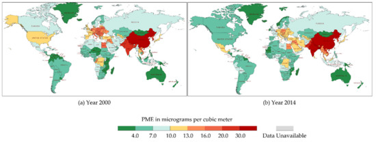
Figure 1.
PME in 2000 and 2014.
Yearly primary energy consumption data from 1980 to 2016 for 230 countries measured in quadrillion British thermal unit (BTU) was downloaded from the website of the Energy Information Administration of the US government [87]. Eliminating ten countries for missing data produced a total of 220 countries, which were matched against 212 countries collected from the Environmental Performance Index website. Finally, 190 countries had matching data between PM2.5 and primary energy consumption during the 2000–2014 period. Thus, the final data set contained 190 countries.
4. Results and Discussion
The results of PRs estimated for the 190 countries from both classical and kinked ECs are ranked from the lowest to the highest PR in Appendix A. Nicaragua is ranked first with the lowest PR of 48.1%, while Ecuador is ranked last with the highest PR of 155.3%. The distribution of PRs for all the 190 countries is displayed in a histogram in Figure 2. The average PR is 96.5% with a standard deviation (SD) of 15.3 and a CV of 15.8. Among the 190 countries, 115 countries (60.5%) exhibited a moderate slope of PR between 90.1% and 110.0%.
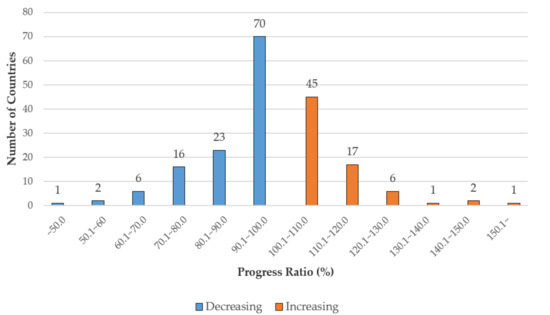
Figure 2.
Progress ratios (PR) of PM2.5 from experience curves (EC) for 190 countries.
Some examples of countries with lower PRs include the 9th-ranked US with a 68.3% slope, the 17th-ranked Japan with a 73.6% slope, and the 19th-ranked United Kingdom with a 76.5% slope. In contrast, the 154th-ranked India with a 106.6% slope and the 180th-ranked Bangladesh with a 119.8% slope are examples of countries with much higher PRs. Accordingly, for each doubling of cumulative energy consumption, the US has generated 31.7% less PME, whereas Bangladesh has generated 19.8% more average PME during the 2000–2014 period.
When the total group of 190 countries was divided into two groups of increasing and decreasing experience slopes, the decreasing group contained 118 countries, ranging from first-ranked Nicaragua with a slope of 48.1% to the 118th-ranked Central African Republic with a slope of 99.7%.
The average PR of the decreasing group was 88.1% with an SD of 10.7 and a CV of 12.1. The increasing group contained 72 countries ranging from the 119th-ranked Aruba with a slope of 100.2% to the 190th-ranked Ecuador with a slope of 155.3%. The average PR for the increasing group was 110.4% with an SD of 10.9 and a CV of 9.8.
Comparing the average PR of the two groups grants an opportunity to propose which of the two groups is more likely to experience further reduction in its experience slope in the future, even though predicting precise levels of PME for individual countries is not attempted here because it requires forecasting future energy consumption of the individual countries. The 118 countries in the group with a decreasing slope in the past would be less likely to experience further reduction in their future slopes simply because they have already made good progress in the past, as evidenced by their average PR of 88.1%. That leaves the group of 72 countries with an increasing slope in the past. Since their average PR is 110.4%, which lagged behind the total average PR of 99.7%, this group is more likely to experience a reduction in the future.
4.1. Classical vs. Kinked
The slope of PR can either remain the same or significantly change. To explore this possibility, both increasing and decreasing groups were tested for whether a shift in the slope has occurred during the 2000–2014 period. This produced four subgroups: Decreasing classical, decreasing kinked, increasing classical, and increasing kinked. To better understand the differences between these four subgroups of countries, EC diagrams are presented in Figure 3. Figure 3a shows the EC for the 50th-ranked Spain representing a decreasing classical slope, while Figure 3b shows the EC for Kuwait representing an increasing classical slope. The value of decreasing classical slope for Spain is −0.15 with R2 of 0.81, while the value of increasing classical slope for the 185th ranked Kuwait is 0.33 with R2 of 0.85. The former represents the PR of 90.2%, while the latter represents the PR of 125.3%.
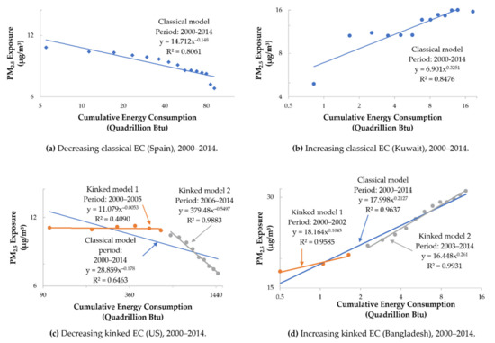
Figure 3.
Four types of EC, 2000–2014.
While a classical EC displays one single slope for the entire period, a kinked EC displays two slopes during the same period. Figure 3c shows the EC for the 9th-ranked US, representing a decreasing kinked slope, while Figure 3d shows the EC for the 180th ranked Bangladesh with an increasing kinked slope. The US displays two slopes—the first slope covering the period of 2000–2005, and the second slope covering the period of 2006–2014. The first kinked slope has a moderate value of −0.01, and the second kinked slope has a steeper value of −0.55. The PR for the second slope is 68.3% with R2 of 0.99, while the first slope is 99.6% with R2 of 0.41. For Bangladesh, the PR from the second kinked slope is 119.8% with an R2 of 0.99, while the PR from the first slope is 107.5% with an R2 of 0.96. In general, the second kinked slope is steeper than the first kinked slope. A kinked year, which begins the second kinked period, also varies by countries. Only the second kinked slope is used to estimate the PR for a given country.
In Figure 4, presenting the distribution of countries in four subgroups, those countries with classical slopes are clustered in the middle with relatively little variation, whereas those with kinked slopes tend to have extreme values on both sides. Among the 118 countries in the decreasing slope group, the 75 countries with classical slopes have the average PR of 93.7% with a very narrow SD of 4.0 and a CV of 4.2, and the 43 countries with kinked slopes have the lowest PR of 78.2% with an SD of 11.5 and a CV of 14.7. Among the 72 countries in the increasing slope group, the 60 countries with classical slopes have the average PR of 107.2% with a narrow SD of 6.1 and a CV of 5.7 and the twelve countries with kinked slopes have the highest PR of 126.4% with an SD of 14.7 and a CV of 11.6. In short, the highest average PR belongs to the twelve countries with increasing kinked slopes, followed by the 60 countries with increasing classical slopes, by the 75 countries with decreasing classical slopes, and finally by the 43 countries with decreasing kinked slopes.
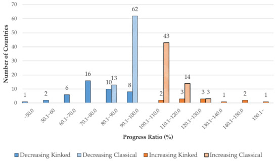
Figure 4.
Four subgroups based on the type of PR.
Based on these results, the future prospect of the PME trend of the four subgroups can be proposed. Among them, the subgroup of 60 countries with an average increasing classical slope of 107.2% may have the best chances of experiencing improvement in their PM2.5 trend in the future. In particular, countries with very high PRs such as Kuwait (PR = 125.3%) and Malaysia (PR = 124.3%) are noteworthy. They are selected because their chances of experiencing a kinked slope with lower PR are more likely given that their PRs are higher than the subgroup’s average of 107.2% and they have not experienced a second slope during the period under analysis.
Next, the subgroup of 12 countries with an increasing kinked slope averaging 126.4% may have the second-best chances for improvement in the future. This group includes countries such as Ecuador (PR = 155.3%), Guatemala (PR = 145.8%), Singapore (PR = 141.5%), Burundi (PR = 136.2%), and Thailand (PR = 127.0%). Even though they have experienced a second experience slope, their chances of encountering a third kinked slope appear good because of very high PRs from their second kinked slopes, which exceed the overall average slope of 190 countries at 96.5% by a wide margin.
The subgroup of 75 countries with a decreasing classical slope may have less chances of improvement than the previous two subgroups in the future because this group has already shown a moderate level of reduction. Finally, the subgroup of 43 countries with a decreasing kinked slope averaging 78.2% may have substantially less chances of experiencing a third kinked slope in the future. The reason is twofold. First, the average kinked slope for this group is the lowest among the four subgroups. This indicates that their past record of improvement stands out to be the best among the four subgroups. Second, they have already experienced two kinked slopes during the period. For these two reasons, they are less likely to experience a steeper third kinked slope in the future.
4.2. Regional Analysis
It is worthwhile to look into the potential differences between the average PR across regions. The World Bank categorizes seven regions of the world from East Asia and Pacific (EAP), Europe and Central Asia (ECA), Latin America and Caribbean (LAC), Middle East and North Africa (MENA), North America (NA), South Asia (SA), and Sub-Saharan Africa (SSA) [88]. Due to the fact that NA contains only 3 countries, NA is combined with ECA to form ECANA. Therefore, six regional subgroups are used in this study: EAP with 28 countries, ECANA with 52 countries, LAC with 36 countries, MENA with 20 countries, SA with eight countries, and finally SSA with 46 countries.
The average PR and the proportion of increasing and decreasing countries vary across six regions (Figure 5). With the exception of ECANA, five of the six regions have a regional average PR higher than the global average of 96.5%. The regional average PR of SA is the highest at 108.5% and that of ECANA is the lowest at 88.7%. The proportion of increasing PR countries also exhibits a wide variation: SA is the highest at 75%, and ECANA is the lowest at 8%. In general, the higher the percentage of increasing PR countries in the region, the higher the region’s average PR. One exception is observed in the case of EAP: Even though SSA’s proportion of increasing PR countries is higher than EAP’s, the regional average PR of the former is lower than that of the latter.
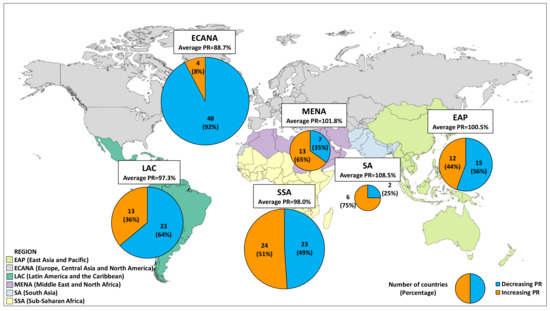
Figure 5.
Regional average PRs and their composition.
4.3. Robustness Test on the Impact of Population
For the investigation of common characteristics among regions that display either an increasing or a decreasing slope, the possible impact of population dynamics among socioeconomic factors has been selected. Figure 6 displays annual measures of population, energy consumption, and the regional average PME during the 2000–2014 period in six regions. While population and energy consumption exhibit, in general, a clear increasing trend, the pace of change shows variation across regions. In some regions, energy consumption increased much faster than population. In SA, for example, population increased 24% from 1.39 billion in 2000 to 1.73 billion in 2014, and energy consumption increased at an even faster pace of 113% from 15 quadrillion BTU in 2000 to 32 quadrillion BTU in 2014. EAP shows a similar pattern: Population increased 11% from 2.06 billion in 2000 to 2.28 billion in 2014 and energy consumption increased 109% from 99 quadrillion BTU in 2000 to 207 quadrillion BTU in 2014. In contrast, the increase in energy consumption during the 2000–2014 period was at a moderate pace of 8% in LAC and ECANA when population increased by 20% in LAC and 7% in ECANA.
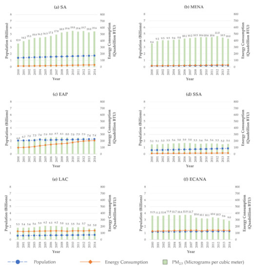
Figure 6.
Change of population, energy consumption, and PME.
The trend of PME displays a pattern different from that of population and energy consumption. While the regional average PME was on the rise to a peak around 2007 to 2010, it generally tends to decrease afterward, even though the amount of decrease varied across regions. First, there is a stark difference in terms of the pace of increase to the peak between the regions with an increasing trend (SA, MENA, and EAP) and those with a decreasing trend (ECANA, LAC, and SSA). In the former case, the regional average PME increased fast since 2000: SA with a 53% increase to 2010, MENA with a 31% increase to 2012, and EAP with a 37% increase to 2007. The latter group had a moderate increase: SSA with a 16% increase to 2006, LAC with a 17% increase to 2007, and ECANA with a 4% increase to 2006. Second, the pace of decrease after the regional peak shows variation as well. While SA had a slight decrease from 2010 to 2014, EAP and SSA showed a substantial decrease of 10% from 2007 to 2014 and 8% from 2006 to 2014, respectively. The case of ECANA is noteworthy: After a stationary level of the regional average of PME from 2000 to 2007, the region exhibited a significant drop of 23% from its peak of 11.7 μg/m3 in 2007 to 9.0 μg/m3 in 2014. In short, the longitudinal impact of population on energy consumption and PME could not be clearly identified.
Additional tests were conducted on the relationship between PR we have estimated and three measures of population dynamics: Population size, percentage change of population size during the 2000–2014 period, and population density. We downloaded population size as well as 2014 population density measures from the U.S. Census Bureau [89]. There were four countries with missing population data so that the total number of countries was reduced from 190 to 186 countries for this robustness test.
4.3.1. Population Size
As shown in Figure 7, the proportion of countries with an increasing slope expands from 0%, or 0 out of eleven countries at 2014 population size of less than 100,000, to 30%, or eight out of 27 countries in the group of countries between 100,000 to one million populations. The proportion expands further to 38%, or 24 out of 64 countries, in the next group of countries between one million to ten million populations. Finally, the proportion increases even further to the high of 47.6% or 40 out of 84 countries in the group of countries with more than ten million populations. In short, the countries with smaller population sizes of less than one million inhabitants are much more likely to display a decreasing slope of PME, whereas the countries with more than 10 million inhabitants face about an even chance of displaying an increasing or a decreasing slope of PME. Furthermore, countries with more than ten million populations account for a majority of 44 countries, or 61% of the 72 countries with an increasing slope. Some of these large population size countries with an increasing slope are led by India, Indonesia, Bangladesh, and Pakistan as shown in Figure 7.
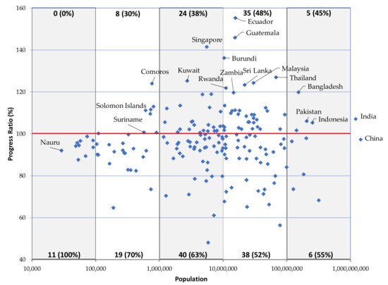
Figure 7.
The relationship between PR and population size (2014) for 186 countries. The numbers at the top and bottom of the figure indicate the number of countries and the percentage in parentheses with increasing and decreasing PRs, respectively, in each population category. In the category of less than 100,000 population, for example, there are eleven countries, all of which had a decreasing PR.
4.3.2. Change of Population Size
When the population size declines during the period of 2000 to 2014, the proportion of the countries with an increasing slope remains low at 13%, or 3 out of 20 countries, as shown in Figure 8. On the other hands, when a rapid expansion of population size takes place with more than 40%, during the period, the proportion of the countries with an increasing slope increases rapidly to 67%, or 6 out of 9 countries. The two other groups of countries with increasing population size between 0% to 20% and 20% to 40% also display higher proportions of countries with an increasing slope at 31% or 28 out of 90 countries and 55% or 35 out of 64 countries, respectively. In summary, a majority of 41, or 57% of the 72 countries with increasing slope, realized more than a 20% increase in their population size during the period of 2000 to 2014. Some of these countries with a rapid population growth with an increasing slope are smaller population countries such as Qatar, UAE, Bahrain, Jordan, and Bermuda.
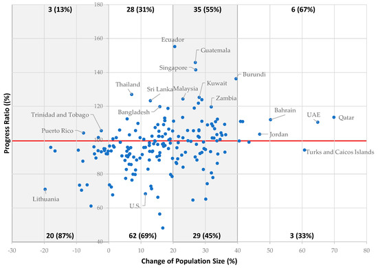
Figure 8.
The relationship between PR and percentage change of population size (2000–2014) for 186 countries. The numbers at the top and the bottom of the figure indicate the number of countries and the percentage in parentheses with an increasing and a decreasing PR, respectively, in the shaded area. For instance, the far left-hand side area with negative population growth included 23 countries, three (or 13%) of which had an increasing PR.
4.3.3. Population Density
Figure 9 shows that the proportion of countries with increasing slope again expands from 31% or five out of 16 countries in the group with the lowest population density of fewer than ten persons per km2 to 43% or six out of 14 countries under the highest population density of more than 500 persons per km2. However, for a majority of the remaining 156 countries between the population density of ten persons to 500 persons per km2, the proportion of countries with an increasing slope remains between 37% to 40%. In other words, the proportion of countries with an increasing slope appears to not be affected significantly by varying population density for a majority of the countries.
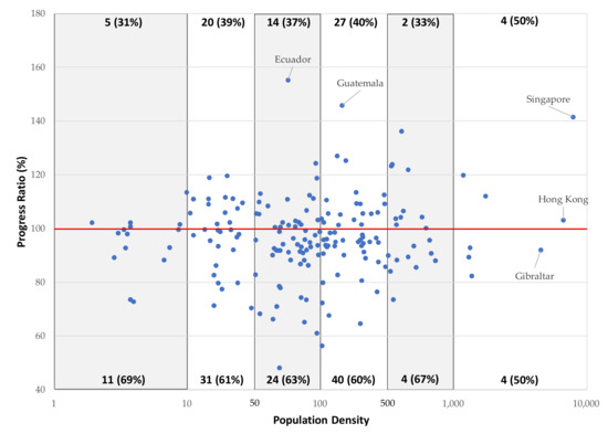
Figure 9.
The relationship between PR and population density (2014) for 186 countries. The numbers at the top and bottom of the figure indicate the number of countries and the percentage in parentheses with an increasing and a decreasing PR, respectively, in each population category. For example, in the category of fewer than ten persons per km2, there are 16 countries, five (or 31%) of which had an increasing PR and eleven (or 69%) a decreasing PR.
In summary, a majority of 44 out of 72 countries (61%) with an increasing slope come from the population size which exceeds ten million inhabitants. Similarly, a majority of 41 out of 72 countries, or 57% of those with an increasing slope, experienced more than a 20% increase in their population sizes during the period of 2000 to 2014. In other words, large population size countries, as well as those countries experiencing a rapid population expansion, are more likely to display an increasing slope. In conclusion, the result of the robustness test indicates that the size of population, as well as the rate of population, change appear to exercise some influence on the slope of PME. On the other hand, population density appears to show almost no influence on the slope of PME.
4.4. Key Findings
The key findings from this research may be summarized as follows. First, the average PR for the total 190 countries is 96.5%, which is close to 100%, where no reduction of PME as a function of doubling the cumulative energy consumption has been achieved. Therefore, the task of reducing PME will be a challenge for the world. However, as PRs for individual countries show a wide variation ranging from 48.1% to 155.3%, the degree of challenge is suggested to vary widely across countries.
Second, a majority of 118 countries displayed a decreasing trend of PME with an average PR of 88.1%. The contribution by the US with a PR of 68.3% and Japan with a PR of 73.6% are some examples of leading countries contributing more toward global reduction of PME. However, the most important finding from this study is that 72 countries, representing 37.9% of the total countries, displayed an increasing trend of PME with a PR of 110.4%, where doubling the cumulative energy consumption has generated a 10.4% increase of PME. This large set of countries experiencing an increasing trend of PME has not been reported earlier, possibly because a majority of previous studies engaged in an intensive investigation of a smaller number of populous and high emission countries.
Third, based on the type of EC, a majority of 135 countries recorded a classical slope with an average PR of 99.7%, but the remaining 55 countries experienced a kinked slope with an average PR of 88.94%. This finding demonstrates the validity of using both classical and kinked ECs. Among the 72 countries displaying an increasing trend of PME, a majority of 60 countries experienced a classical slope, while 12 countries displayed a kinked slope. Our analysis indicates that those 60 countries with an increasing classical slope seem to have the best chances of substantial improvement in their future PME trend. The remaining 12 countries with an increasing kinked slope may also have some chances of improvement in their future trend. Among the 118 countries experiencing a decreasing trend, 75 countries displayed a classical slope, while 43 countries displayed a kinked slope. The subgroup of 75 countries with a decreasing classical slope may have substantially less chances of improvement in their future trend, as they have already learned to manage their future PME more effectively.
Fourth, big differences were observed across six regions of the world, ranging from Europe, Central Asia and North America’s 88.7% to East Asia and Pacific’s 110.1%. Three regions in particular should be noticed due to their PRs higher than the overall average: East Asia and Pacific, South Asia, and Middle East and North Africa. From the three regions, ten countries, each with a PR higher than its subgroup average, may have better chances of improvement in the future: Two countries in East Asia and Pacific, two countries in South Asia, and six countries in Middle East and North Africa.
Fifth, countries with larger population sizes of more than ten million inhabitants are more likely to display an increasing slope. For example, as many as 38 out of the 82 countries with more than ten million people have displayed an increasing slope, as summarized in Table 2. The SSA region has provided the highest number of 17 large population countries displaying an increasing slope out of the total of 27 countries in this population category. The SA region has provided three countries displaying an increasing slope out of the total of three countries. EAP, LAC, and MENA regions produced six, six, and four countries each with an increasing slope, while the remaining two countries with increasing slopes came from the ECANA region. In other words, 38 out of 82 countries, or 46% of the total, displayed an increasing slope, whereas 44 out of 84 countries or 54% displayed a decreasing slope in this large population category.
Table 2.
Region, population size, and PR.
In the next group of countries with the population size between one to ten million, 26 out of 67 countries, or 39%, have displayed an increasing slope. The MENA region produced eight out of nine countries with an increasing slope, while the LAC region produced five countries out of the total of eleven countries with an increasing slope as well. SSA and EAP also contributed five and four countries each with an increasing slope, making the total number of countries with an increasing slope at 24 countries. Two additional countries from ECANA brought the total number at 26 countries with an increasing slope, or 39%, out of the total 67 countries in the medium-size population category.
Finally, there are 37 countries with population sizes of less than one million inhabitants. This group contributed only eight countries, or 22% of the total, with an increasing slope. EAP, LAC and SSA contributed two countries each, while MENA and SA generated one country each. Unlike the other five regions, the ECANA region contributed only four countries with an increasing slope out of the total of 51 countries across varying population sizes. In other words, the ECANA region has generated 47 countries or 92% of the total 51 countries displaying a decreasing slope.
In summary, the group of large population size countries contributed 38 countries, or 53% of the total of 72 countries with an increasing slope, was helped especially by the SSA and SA regions. The group of medium-population countries contributed 26 countries, or 36% to the total 72 countries with an increasing slope, helped especially by the MENA and LAC regions. Finally, the group of small-population countries contributed only eight countries, or 11% of the total with an increasing slope. On the other hand, ENCANA region contributed as many as 47 countries with a decreasing slope across varying population sizes, particularly from a majority of countries coming from the population size with more than one million inhabitants.
5. Conclusions
Ambient air pollution generates economic, social, and health issues all over the world. Understanding the phenomenon on a global scale is required to properly deal with this. This study is an attempt to fill a gap in the literature by comparing the trend of PME change during the 2000–2014 period across 190 countries. More specifically, the PR of an EC is employed to identify those countries whose PME increases/decreases as their cumulative energy consumption doubles. While the average PR for 190 countries was 96.5%, a moderate decreasing trend for each doubling of the cumulative energy consumption, two groups were identified: 118 countries showing a decreasing trend with an average PR of 88.1%, and 72 countries showing an increasing trend with an average PR of 110.4%. Using two types of EC, classical and kinked, demonstrated that some countries experienced a significant shift in slope: 36.4% of the countries with a decreasing trend and 16.7% of the countries with an increasing trend. Regional differences in terms of an average PR were found as well: All regions except ECANA had an average PR higher than the overall global average of 96.5%.
The contribution of this research to the literature is across two dimensions. First, this may be the first application of EC to estimate PRs of PME in 190 countries by using the cumulative primary energy consumption as an independent variable. As in the CO2 emissions research, EC has the potential to be a useful tool to understand the trend of PME across multiple groups of countries. For example, by using both classical and kinked EC, it was discovered that as many as 55 countries displayed a kinked slope, which demonstrates that the rates of change expressed in PRs are not constant and are subject to change during the period.
Second, the variation of PRs identified through the subgroup analysis suggests that different approaches to reducing PMEs are needed depending on the subgroup a country belongs to. As some countries from the three subgroups of 147 countries—increasing classical, increasing kinked, and decreasing classical slope—may migrate to join the decreasing kinked subgroup in the future, the average PRs for the 190 countries may gradually decrease. One critical success factor in this context will include a more rapid reduction of PRs, possibly by populous and high-emission countries such as China, India, Pakistan, Bangladesh, Indonesia, and many others. In addition, international cooperation and assistance extended to emerging countries can help them catch up more rapidly with leading countries of decreasing kinked slope in the management of PME.
The two subgroups—the 60 countries with an increasing classical slope and the twelve countries with an increasing kinked slope—deserve particular attention. More specifically, a majority of 52%, or 38 out of the 72 countries with an increasing slope, had larger population sizes of more than ten million inhabitants, and many of these countries came from the SSA, EAP, and LAC regions. These 72 countries should realize that some of their PRs may be more likely to remain constant and that they are more likely to experience reduced slopes for their PME in the future. Therefore, they should be prepared to take advantage of the forthcoming opportunity by doubling their efforts to control PME across all fronts. Benchmarking the leading countries with lower PRs in the comparable subgroup could help identify key critical success factors to reduce PRs. While the question of how much reduction in PR can be realized by these countries cannot be predicted accurately, the average PR of 78.2% from the decreasing kinked subgroup of 43 countries may serve as an ultimate target to be achieved in the future, particularly for the 60 countries with an increasing classical slope. As for the 75 countries with a decreasing classical slope, some of these countries may experience somewhat reduced PRs in their future. Once again, their current classical slopes can be replaced by steeper kinked slopes. They can also use the average PR of 78.2% of the decreasing kinked subgroup as their possible benchmark target.
There are several limitations to this research involving both conceptual and technical issues. Conceptually, the PME is a function of many interacting socioeconomic variables, such as population, income, economic growth rate, energy consumption structure, industrial structure, urbanization density, private vehicle, coal consumption, international trade, weather, and many others [13,17,18,25,82,83,84,85,86]. However, in this study, the PME of different countries are evaluated only in terms of macro factors such as slope and region. Therefore, future studies of extending customized policy implications for individual as well as regional groups of countries by incorporating such local issues as energy, coal, traffic, transportation, manufacturing, services and many others are suggested. Technically, as the model used in this study is a simple aggregate EC driven by a single independent variable of cumulative primary energy consumption, this study leaves room for further refinement.
To conclude, this research should be viewed as the first step toward a comprehensive understanding of the wide variation of PME among multiple countries. It is also important to note that future studies should definitely focus on countries experiencing an increasing slope of PME, as these countries are likely to drive future improvement of PME in the world.
Author Contributions
The authors contributed to the development, implementation, analysis, and writing of this study as follows: Conceptualization, methodology, and analysis—Y.S.C.; original draft preparation—Y.S.C. and H.E.K.; review and editing—Y.S.C., H.E.K. and B.-J.Y. All authors have read and agreed to the published version of the manuscript.
Funding
The research received no external funding.
Acknowledgments
The authors are very grateful for an anonymous reviewer, who suggested many ideas to improve the quality of the paper, especially the idea to investigate the role of population. Competent help provided by research assistants, SanHa Shin, SeongMin Son, and KyoungHoon Jeon, at the Gachon Center for Convergence Research is appreciated.
Conflicts of Interest
The authors declare no conflict of interest.
Appendix A
Table A1.
Classical and kinked EC for PM2.5 of 190 countries, 2000–2014.
Table A1.
Classical and kinked EC for PM2.5 of 190 countries, 2000–2014.
| Classical Experience Eq | Kinked Year | Kinked Experience Eq | Model Selection | Selected PR | ||||||||||
|---|---|---|---|---|---|---|---|---|---|---|---|---|---|---|
| Country | ln a | b | R_sq | PR | ln a1 | b1 | ln a2 | b2 | b2-b1 | R_sq | PR2 | |||
| 1. Nicaragua | 1.450*** (0.054) | −0.010 (0.040) | 0.007 | 0.993 | 2011 | 1.566*** (0.041) | 0.059 (0.043) | 1.278*** (0.020) | −1.055* (0.293) | −1.115*** (0.296) | 0.752 | 0.481 | Kinked | 0.481 |
| 2. Turkey | 2.376*** (0.075) | 0.024 (0.025) | 0.134 | 1.017 | 2012 | 2.311*** (0.038) | 0.051*** (0.013) | 5.748*** (0.058) | −0.827** (0.014) | −0.878*** (0.020) | 0.772 | 0.564 | Kinked | 0.564 |
| 3. Swaziland | 1.865*** (0.073) | 0.034 (0.026) | 0.101 | 1.024 | 2010 | 1.987*** (0.114) | 0.077 (0.050) | 0.646* (0.252) | −0.777** (0.167) | −0.854*** (0.174) | 0.714 | 0.584 | Kinked | 0.584 |
| 4. Serbia | 2.863*** (0.053) | −0.182*** (0.043) | 0.749 | 0.882 | 2011 | 2.863*** (0.098) | −0.210* (0.101) | 3.740*** (0.325) | −0.711* (0.193) | −0.501* (0.218) | 0.900 | 0.611 | Kinked | 0.611 |
| 5. Sao Tome and Principe | 0.832*** (0.261) | −0.098 (0.058) | 0.175 | 0.934 | 2005 | 1.378 (0.831) | 0.014 (0.155) | −1.274** (0.427) | −0.629*** (0.105) | −0.643*** (0.187) | 0.838 | 0.647 | Kinked | 0.647 |
| 6. Cote d’Ivoire | 1.765*** (0.048) | −0.043 (0.062) | 0.044 | 0.970 | 2006 | 1.935*** (0.168) | 0.128 (0.232) | 1.924*** (0.027) | −0.618*** (0.094) | −0.745** (0.250) | 0.790 | 0.652 | Kinked | 0.652 |
| 7. South Africa | 1.695*** (0.051) | 0.031* (0.017) | 0.171 | 1.021 | 2010 | 1.669*** (0.047) | 0.039** (0.015) | 4.359*** (0.499) | −0.594** (0.117) | −0.632*** (0.118) | 0.705 | 0.663 | Kinked | 0.663 |
| 8. Portugal | 2.455*** (0.145) | −0.217*** (0.067) | 0.726 | 0.861 | 2007 | 2.293*** (0.008) | −0.060*** (0.006) | 3.287*** (0.246) | −0.563*** (0.101) | −0.503*** (0.101) | 0.960 | 0.677 | Kinked | 0.677 |
| 9. United States | 3.362*** (0.483) | −0.178** (0.072) | 0.646 | 0.884 | 2006 | 2.405*** (0.063) | −0.005 (0.012) | 5.939*** (0.415) | −0.550*** (0.058) | −0.544*** (0.060) | 0.988 | 0.683 | Kinked | 0.683 |
| 10. Estonia | 1.984*** (0.026) | −0.022 (0.024) | 0.057 | 0.985 | 2008 | 1.989*** (0.031) | −0.012 (0.023) | 2.017*** (0.027) | −0.505** (0.186) | −0.493** (0.187) | 0.671 | 0.705 | Kinked | 0.705 |
| 11. Lithuania | 2.572*** (0.027) | −0.084** (0.031) | 0.359 | 0.944 | 2006 | 2.568*** (0.016) | −0.036 (0.041) | 3.086*** (0.107) | −0.494*** (0.088) | −0.458*** (0.097) | 0.819 | 0.710 | Kinked | 0.710 |
| 12. Argentina | 1.741*** (0.070) | −0.027 (0.026) | 0.085 | 0.981 | 2008 | 1.651*** (0.047) | 0.012 (0.019) | 3.406*** (0.320) | −0.488*** (0.091) | −0.500*** (0.093) | 0.829 | 0.713 | Kinked | 0.713 |
| 13. Cuba | 1.454*** (0.048) | −0.147*** (0.047) | 0.597 | 0.903 | 2006 | 1.449*** (0.023) | −0.027 (0.052) | 1.891*** (0.082) | −0.467*** (0.073) | −0.440*** (0.090) | 0.911 | 0.723 | Kinked | 0.723 |
| 14. Canada | 2.606*** (0.296) | −0.125* (0.063) | 0.500 | 0.917 | 2006 | 2.013*** (0.103) | 0.044 (0.025) | 4.249*** (0.259) | −0.458*** (0.053) | −0.502*** (0.059) | 0.981 | 0.728 | Kinked | 0.728 |
| 15. Ukraine | 2.958*** (0.269) | −0.095 (0.070) | 0.310 | 0.936 | 2008 | 2.537*** (0.038) | 0.057*** (0.012) | 4.378*** (0.646) | −0.445** (0.155) | −0.502*** (0.155) | 0.927 | 0.735 | Kinked | 0.735 |
| 16. Guyana | 0.685 (0.623) | −0.029 (0.379) | 0.004 | 0.980 | 2002 | 7.115*** (1.301) | 1.924*** (0.408) | 0.023 (0.182) | −0.443*** (0.098) | −2.367*** (0.419) | 0.901 | 0.736 | Kinked | 0.736 |
| 17. Japan | 2.629*** (0.216) | −0.026 (0.042) | 0.084 | 0.983 | 2008 | 2.340*** (0.089) | 0.044** (0.020) | 4.921*** (0.165) | −0.442*** (0.030) | −0.486*** (0.036) | 0.912 | 0.736 | Kinked | 0.736 |
| 18. Senegal | 1.542*** (0.044) | −0.080* (0.040) | 0.268 | 0.946 | 2006 | 1.714*** (0.182) | 0.030 (0.151) | 1.490*** (0.032) | −0.428*** (0.078) | −0.458** (0.170) | 0.740 | 0.743 | Kinked | 0.743 |
| 19. United Kingdom | 3.085*** (0.323) | −0.188** (0.073) | 0.715 | 0.878 | 2003 | 2.479*** (0.200) | 0.004 (0.064) | 3.984*** (0.130) | −0.387*** (0.030) | −0.391*** (0.071) | 0.970 | 0.765 | Kinked | 0.765 |
| 20. Finland | 1.723*** (0.066) | 0.007 (0.031) | 0.004 | 1.005 | 2006 | 1.625*** (0.077) | 0.077 (0.050) | 2.707*** (0.092) | −0.368*** (0.037) | −0.445*** (0.062) | 0.908 | 0.775 | Kinked | 0.775 |
| 21. Cameroon | 1.939*** (0.052) | 0.073 (0.052) | 0.190 | 1.052 | 2006 | 2.110*** (0.110) | 0.202** (0.084) | 1.957*** (0.021) | −0.359*** (0.067) | −0.561*** (0.108) | 0.868 | 0.780 | Kinked | 0.780 |
| 22. Panama | 1.032*** (0.113) | −0.028 (0.145) | 0.016 | 0.981 | 2004 | 1.264*** (0.099) | 0.351 (0.240) | 1.316*** (0.060) | −0.349*** (0.088) | −0.700** (0.255) | 0.765 | 0.785 | Kinked | 0.785 |
| 23. Paraguay | 1.720*** (0.090) | −0.081 (0.073) | 0.234 | 0.946 | 2008 | 1.702*** (0.018) | 0.086*** (0.025) | 2.056*** (0.224) | −0.327* (0.150) | −0.413** (0.152) | 0.875 | 0.797 | Kinked | 0.797 |
| 24. Sweden | 2.130*** (0.106) | −0.071* (0.039) | 0.279 | 0.952 | 2008 | 1.917*** (0.129) | 0.047 (0.053) | 2.923*** (0.389) | −0.326** (0.121) | −0.373** (0.132) | 0.857 | 0.798 | Kinked | 0.798 |
| 25. France | 2.715*** (0.099) | −0.069** (0.023) | 0.549 | 0.953 | 2008 | 2.519*** (0.085) | −0.012 (0.021) | 3.941*** (0.232) | −0.324*** (0.049) | −0.312*** (0.053) | 0.93 | 0.799 | Kinked | 0.799 |
| 26. Nigeria | 1.910*** (0.105) | 0.129** (0.056) | 0.489 | 1.093 | 2007 | 1.799*** (0.050) | 0.260*** (0.034) | 2.920*** (0.270) | −0.310** (0.122) | −0.569*** (0.127) | 0.930 | 0.807 | Kinked | 0.807 |
| 27. Malta | 1.892*** (0.044) | −0.117* (0.063) | 0.516 | 0.922 | 2004 | 2.249*** (0.049) | 0.073** (0.029) | 1.841*** (0.032) | −0.279*** (0.050) | −0.353*** (0.058) | 0.842 | 0.824 | Kinked | 0.824 |
| 28. Belize | 0.671*** (0.108) | −0.274*** (0.037) | 0.707 | 0.827 | 2004 | 0.394 (0.860) | −0.324 (0.222) | −0.032 (0.235) | −0.576*** (0.106) | −0.2519 (0.246) | 0.884 | 0.671 | Classical | 0.827 |
| 29. Denmark | 2.547*** (0.104) | −0.129** (0.054) | 0.591 | 0.914 | 2003 | 2.449*** (0.019) | −0.001 (0.026) | 2.848*** (0.074) | −0.274*** (0.045) | −0.272*** (0.052) | 0.822 | 0.827 | Kinked | 0.827 |
| 30. Bahamas, The | 1.303*** (0.118) | −0.272** (0.095) | 0.616 | 0.828 | 2013 | 1.463*** (0.053) | −0.181*** (0.042) | 1.065 (0.472) | 0.000 (1.410) | 0.181 (13.497) | 0.948 | 1.000 | Classical | 0.828 |
| 31. Philippines | 1.614*** (0.269) | 0.117 (0.119) | 0.334 | 1.084 | 2006 | 1.392*** (0.265) | 0.323* (0.169) | 2.516*** (0.216) | −0.250** (0.089) | −0.573** (0.191) | 0.846 | 0.841 | Kinked | 0.841 |
| 32. Korea, South | 3.096*** (0.140) | −0.008 (0.033) | 0.009 | 0.995 | 2009 | 2.830*** (0.048) | 0.076*** (0.013) | 4.087*** (0.491) | −0.224* (0.100) | −0.300** (0.101) | 0.938 | 0.856 | Kinked | 0.856 |
| 33. Guam | 0.640** (0.233) | −0.222 (0.160) | 0.232 | 0.858 | 2013 | 0.959*** (0.026) | −0.054** (0.019) | 0.095 (0.130) | 0.000 (0.250) | 0.054 (1.914) | 0.990 | 1.000 | Classical | 0.858 |
| 34. Algeria | 2.205*** (0.106) | −0.061 (0.043) | 0.354 | 0.958 | 2006 | 2.046*** (0.049) | 0.071** (0.028) | 2.613*** (0.088) | −0.214*** (0.034) | −0.285*** (0.044) | 0.937 | 0.862 | Kinked | 0.862 |
| 35. Sierra Leone | 1.104*** (0.246) | −0.213** (0.090) | 0.641 | 0.863 | 2008 | 1.855*** (0.122) | −0.025 (0.033) | 0.821 (0.438) | −0.300 (0.184) | −0.275 (0.187) | 0.953 | 0.812 | Classical | 0.863 |
| 36. Ireland | 1.990*** (0.083) | −0.204*** (0.059) | 0.622 | 0.868 | 2012 | 1.945*** (0.037) | −0.133*** (0.022) | 7.000 (3.810) | −2.587 (1.755) | −2.454 (1.755) | 0.908 | 0.166 | Classical | 0.868 |
| 37. Cape Verde | 0.980*** (0.280) | −0.198** (0.080) | 0.461 | 0.872 | 2013 | 1.379*** (0.101) | −0.098*** (0.028) | 0.916 (1.042) | 0.000 (0.522) | 0.098 (0.456) | 0.934 | 1.000 | Classical | 0.872 |
| 38. American Samoa | 0.503 (0.545) | −0.191 (0.161) | 0.143 | 0.876 | 2013 | 1.244*** (0.021) | 0.007 (0.008) | 0.095 (0.048) | 0.000 (0.022) | −0.007 (0.041) | 1.000 | 1.000 | Classical | 0.876 |
| 39. Taiwan | 2.556*** (0.170) | 0.036 (0.049) | 0.141 | 1.025 | 2005 | 2.320*** (0.125) | 0.138** (0.047) | 3.378*** (0.095) | −0.183*** (0.027) | −0.321*** (0.055) | 0.867 | 0.881 | Kinked | 0.881 |
| 40. Morocco | 2.055*** (0.022) | −0.064*** (0.017) | 0.510 | 0.957 | 2008 | 2.043*** (0.029) | 0.001 (0.038) | 2.247*** (0.076) | −0.181** (0.046) | −0.182** (0.060) | 0.833 | 0.882 | Kinked | 0.882 |
| 41. Belgium | 2.850*** (0.056) | −0.036* (0.020) | 0.226 | 0.975 | 2005 | 2.749*** (0.174) | 0.013 (0.077) | 3.329*** (0.156) | 0.180*** (0.050) | −0.192* (0.092) | 0.644 | 0.883 | Kinked | 0.883 |
| 42. Guinea−Bissau | 1.090*** (0.190) | −0.180*** (0.054) | 0.687 | 0.883 | 2008 | 1.632*** (0.096) | −0.061** (0.022) | 0.953 (0.761) | −0.209 (0.246) | −0.147 (0.247) | 0.876 | 0.865 | Classical | 0.883 |
| 43. Kazakhstan | 1.906*** (0.070) | 0.029 (0.023) | 0.099 | 1.020 | 2005 | 1.779*** (0.202) | 0.089 (0.102) | 2.604*** (0.090) | −0.180*** (0.026) | −0.269** (0.105) | 0.827 | 0.883 | Kinked | 0.883 |
| 44. Luxembourg | 2.568*** (0.021) | −0.169*** (0.023) | 0.759 | 0.890 | 2011 | 2.544*** (0.024) | −0.201*** (0.023) | 3.314* (0.970) | −0.921 (1.062) | −0.721 (1.062) | 0.860 | 0.528 | Classical | 0.890 |
| 45. Namibia | 1.589*** (0.009) | −0.165*** (0.011) | 0.964 | 0.892 | 2002 | 1.848 (7.653) | −0.082 (2.500) | 1.605*** (0.009) | −0.140*** (0.012) | −0.058 (2.500) | 0.987 | 0.907 | Classical | 0.892 |
| 46. Bermuda | 0.173 (0.211) | −0.162** (0.068) | 0.480 | 0.894 | 2012 | 0.367*** (0.081) | −0.109*** (0.030) | −14.420 (3.203) | −7.189 (1.543) | −7.081*** (0.477) | 0.885 | 0.007 | Classical | 0.894 |
| 47. Nauru | 0.474 (0.675) | −0.161 (0.141) | 0.199 | 0.895 | 2013 | 1.312*** (0.115) | −0.001 (0.025) | 0.531 (0.424) | 0.000 (0.114) | 0.001 (0.190) | 0.981 | 1.000 | Classical | 0.895 |
| 48. Grenada | 0.159 (0.494) | −0.152 (0.112) | 0.170 | 0.900 | 2013 | 0.859*** (0.167) | 0.001 (0.040) | −8.189 (4.441) | −2.803 (1.503) | −2.804*** (0.052) | 0.934 | 0.143 | Classical | 0.900 |
| 49. Guinea | 1.567*** (0.120) | −0.150* (0.082) | 0.412 | 0.901 | 2008 | 2.115*** (0.058) | 0.063** (0.026) | 1.387*** (0.136) | −0.246 (0.137) | −0.310** (0.139) | 0.928 | 0.843 | Classical | 0.901 |
| 50. Spain | 2.689*** (0.143) | −0.148*** (0.038) | 0.806 | 0.902 | 2012 | 2.596*** (0.094) | −0.116*** (0.025) | 7.625 (3.434) | −1.274 (0.771) | 1.158 (0.772) | 0.952 | 0.414 | Classical | 0.902 |
| 51. Tonga | −0.4454 (0.654) | −0.150 (0.138) | 0.148 | 0.902 | 2013 | 0.415*** (0.082) | 0.018 (0.019) | −0.511 (0.824) | −0.000 (0.229) | −0.018 (0.148) | 0.998 | 1.000 | Classical | 0.902 |
| 52. Slovenia | 2.792*** (0.052) | −0.141** (0.053) | 0.473 | 0.907 | 2008 | 2.843*** (0.017) | 0.016 (0.037) | 2.576*** (0.314) | −0.026 (0.264) | −0.043 (0.267) | 0.898 | 0.982 | Classical | 0.907 |
| 53. Barbados | 0.812** (0.308) | −0.140 (0.141) | 0.122 | 0.908 | 2013 | 1.253*** (0.051) | 0.033 (0.023) | 1.499 (0.224) | 1.192 (0.223) | 1.158*** (0.196) | 0.970 | 2.284 | Classical | 0.908 |
| 54. French Polynesia | −0.1864 (0.387) | −0.137 (0.139) | 0.121 | 0.909 | 2013 | 0.350*** (0.037) | 0.033** (0.014) | −0.693 (0.031) | 0.000 (0.021) | −0.033 (0.352) | 0.995 | 1.000 | Classical | 0.909 |
| 55. Tajikistan | 2.299*** (0.018) | 0.104*** (0.022) | 0.743 | 1.074 | 2008 | 2.281*** (0.021) | 0.081 (0.061) | 2.536*** (0.053) | −0.132* (0.061) | −0.214** (0.086) | 0.859 | 0.912 | Kinked | 0.912 |
| 56. Italy | 3.201*** (0.162) | −0.131*** (0.039) | 0.666 | 0.913 | 2008 | 2.901*** (0.061) | −0.030 (0.018) | 3.335*** (0.590) | −0.170 (0.133) | −0.140 (0.135) | 0.944 | 0.889 | Classical | 0.913 |
| 57. Samoa | −0.366 (0.689) | −0.128 (0.164) | 0.093 | 0.915 | 2013 | 0.565*** (0.068) | 0.076*** (0.018) | −0.693 (0.563) | 0.000 (0.187) | −0.076 (10.518) | 0.994 | 1.000 | Classical | 0.915 |
| 58. Yemen | 2.278*** (0.019) | 0.043* (0.023) | 0.498 | 1.030 | 2007 | 2.283*** (0.009) | 0.063 (0.039) | 2.465*** (0.041) | −0.123** (0.035) | −0.185*** (0.052) | 0.834 | 0.918 | Kinked | 0.918 |
| 59. Belarus | 2.880*** (0.081) | −0.122*** (0.040) | 0.571 | 0.919 | 2008 | 2.768*** (0.035) | −0.015 (0.026) | 3.224*** (0.384) | −0.273 (0.152) | −0.257 (0.154) | 0.849 | 0.828 | Classical | 0.919 |
| 60. Croatia | 2.798*** (0.062) | −0.120** (0.051) | 0.481 | 0.920 | 2008 | 2.803*** (0.014) | 0.017 (0.018) | 2.641*** (0.219) | −0.059 (0.148) | −0.076 (0.150) | 0.934 | 0.96 | Classical | 0.920 |
| 61. Gibraltar | 1.962*** (0.022) | −0.120*** (0.025) | 0.664 | 0.920 | 2012 | 1.970*** (0.018) | −0.109*** (0.015) | 3.789 (1.500) | −2.258 (1.718) | −2.150 (1.718) | 0.866 | 0.209 | Classical | 0.920 |
| 62. Montenegro | 2.311*** (0.101) | −0.121* (0.059) | 0.607 | 0.920 | 2013 | 2.398*** (0.060) | −0.081* (0.033) | 0.880 (11.082) | −1.704 (12.254) | −1.623 (1.237) | 0.880 | 0.307 | Classical | 0.920 |
| 63. Vanuatu | 0.047 (0.248) | −0.119* (0.058) | 0.624 | 0.921 | 2005 | 0.813* (0.397) | 0.015 (0.075) | 0.272 (0.272) | −0.057 (0.068) | −0.072 (0.101) | 0.902 | 0.961 | Classical | 0.921 |
| 64. Colombia | 1.132* (0.532) | 0.147 (0.220) | 0.241 | 1.107 | 2002 | 0.355 (0.458) | 1.293 (0.773) | 1.755*** (0.091) | −0.111** (0.036) | −1.404* (0.774) | 0.981 | 0.926 | Kinked | 0.926 |
| 65. Mauritania | 1.030*** (0.059) | −0.108*** (0.029) | 0.565 | 0.928 | 2003 | 0.756* (0.374) | −0.164 (0.114) | 0.849*** (0.064) | −0.230*** (0.030) | −0.066 (0.118) | 0.871 | 0.853 | Classical | 0.928 |
| 66. Gabon | 1.684*** (0.076) | −0.049 (0.075) | 0.148 | 0.967 | 2002 | 2.960*** (0.858) | 0.405 (0.273) | 1.629*** (0.053) | −0.106** (0.035) | −0.510* (0.275) | 0.585 | 0.929 | Kinked | 0.929 |
| 67. Maldives | −0.6522** (0.277) | −0.106 (0.093) | 0.175 | 0.929 | 2013 | −0.243** (0.086) | 0.015 (0.028) | −0.916 (1.151) | 0.000 (0.761) | −0.015 (0.087) | 0.926 | 1.000 | Classical | 0.929 |
| 68. Ethiopia | 1.836*** (0.018) | 0.031** (0.014) | 0.293 | 1.022 | 2006 | 1.863*** (0.065) | 0.056 (0.049) | 1.852*** (0.008) | −0.102*** (0.025) | −0.157** (0.055) | 0.853 | 0.932 | Kinked | 0.932 |
| 69. Hungary | 3.040*** (0.091) | −0.102** (0.044) | 0.419 | 0.932 | 2008 | 2.914*** (0.062) | 0.027 (0.038) | 3.258*** (0.462) | −0.211 (0.191) | −0.238 (0.195) | 0.889 | 0.864 | Classical | 0.932 |
| 70. Tunisia | 2.151*** (0.069) | −0.101 (0.064) | 0.464 | 0.932 | 2002 | 2.166*** (0.363) | 0.032 (0.347) | 2.286*** (0.028) | −0.225*** (0.031) | −0.256 (0.349) | 0.825 | 0.856 | Classical | 0.932 |
| 71. Norway | 1.793*** (0.192) | −0.099 (0.071) | 0.319 | 0.934 | 2008 | 1.541*** (0.033) | 0.055** (0.018) | 2.278** (0.640) | −0.274 (0.208) | −0.329 (0.209) | 0.843 | 0.827 | Classical | 0.934 |
| 72. Netherlands | 2.995*** (0.091) | −0.098*** (0.028) | 0.601 | 0.935 | 2013 | 2.918*** (0.042) | −0.068*** (0.013) | 4.643 (0.275) | −0.527 (0.067) | −0.459 (1.364) | 0.870 | 0.694 | Classical | 0.935 |
| 73. Poland | 3.135*** (0.213) | −0.097 (0.063) | 0.338 | 0.935 | 2008 | 2.805*** (0.050) | 0.052** (0.020) | 3.323*** (0.604) | −0.163 (0.164) | −0.215 (0.165) | 0.849 | 0.893 | Classical | 0.935 |
| 74. Macedonia | 2.665*** (0.030) | −0.095** (0.034) | 0.463 | 0.936 | 2008 | 2.791*** (0.021) | 0.003 (0.031) | 2.667*** (0.040) | −0.261 (0.193) | −0.2642 (0.196) | 0.789 | 0.834 | Classical | 0.936 |
| 75. Seychelles | −0.601** (0.270) | −0.096 (0.099) | 0.114 | 0.936 | 2013 | −0.232** (0.078) | 0.210 (0.028) | −0.916 (0.926) | 0.000 (0.572) | −0.021 (0.343) | 0.928 | 1.000 | Classical | 0.936 |
| 76. Slovakia | 2.918*** (0.066) | −0.095** (0.036) | 0.464 | 0.936 | 2008 | 2.842*** (0.044) | 0.007 (0.029) | 2.933*** (0.455) | −0.122 (0.211) | −0.128 (0.213) | 0.852 | 0.919 | Classical | 0.936 |
| 77. Moldova | 2.642*** (0.020) | −0.094*** (0.030) | 0.589 | 0.937 | 2008 | 2.722*** (0.018) | −0.026* (0.014) | 2.630*** (0.062) | −0.138 (0.171) | −0.112 (0.171) | 0.804 | 0.909 | Classical | 0.937 |
| 78. Romania | 2.956*** (0.134) | −0.092 (0.054) | 0.369 | 0.938 | 2008 | 2.788*** (0.032) | 0.025 (0.015) | 3.584*** (0.697) | −0.322 (0.243) | −0.347 (0.243) | 0.829 | 0.800 | Classical | 0.938 |
| 79. Armenia | 2.585*** (0.032) | 0.083 (0.090) | 0.267 | 1.059 | 2003 | 3.090*** (0.169) | 0.410*** (0.109) | 2.598*** (0.019) | −0.091** (0.037) | −0.500*** (0.115) | 0.855 | 0.939 | Kinked | 0.939 |
| 80. Bulgaria | 2.818*** (0.069) | −0.088** (0.038) | 0.426 | 0.941 | 2008 | 2.739*** (0.052) | 0.021 (0.035) | 3.134*** (0.304) | −0.249 (0.141) | −0.269* (0.146) | 0.895 | 0.842 | Classical | 0.941 |
| 81. Turks and Caicos Islands | 1.227*** (0.314) | −0.086 (0.064) | 0.168 | 0.942 | 2013 | 1.659*** (0.245) | −0.002 (0.057) | −4.686 (4.225) | −1.719 (1.232) | −1.717*** (0.404) | 0.806 | 0.304 | Classical | 0.942 |
| 82. Cayman Islands | 1.052*** (0.209) | −0.081 (0.061) | 0.180 | 0.945 | 2013 | 1.350*** (0.035) | −0.002( 0.009) | 0.916 (1.020) | −0.000 (0.486) | 0.002 (0.356) | 0.949 | 1.000 | Classical | 0.945 |
| 83. Saint Lucia | 0.552 (0.413) | −0.077 (0.103) | 0.047 | 0.948 | 2013 | 1.185*** (0.236) | 0.079 (0.076) | −2.678 (0.143) | −1.143 (0.059) | −1.223*** (0.153) | 0.911 | 0.453 | Classical | 0.948 |
| 84. Greece | 2.627*** (0.068) | −0.075** (0.032) | 0.439 | 0.949 | 2013 | 2.585*** (0.034) | −0.046*** (0.014) | 10.527 (6.647) | −2.782 (2.249) | −2.736*** (0.342) | 0.863 | 0.145 | Classical | 0.949 |
| 85. Germany | 2.990*** (0.193) | −0.074* (0.041) | 0.305 | 0.950 | 2008 | 2.567*** (0.161) | 0.044 (0.038) | 2.954** (0.738) | −0.077 (0.147) | −0.121 (0.152) | 0.854 | 0.948 | Classical | 0.950 |
| 86. Gambia, The | 1.329*** (0.151) | −0.073 (0.046) | 0.323 | 0.951 | 2003 | 1.751** (0.602) | 0.028 (0.131) | 0.927*** (0.118) | −0.208*** (0.033) | −0.237 (0.135) | 0.743 | 0.866 | Classical | 0.951 |
| 87. Kiribati | −0.8631 (0.556) | −0.073 (0.103) | 0.053 | 0.951 | 2013 | −0.048 (0.063) | 0.071*** (0.014) | −1.204 (0.497) | 0.000 (0.128) | −0.071 (0.299) | 0.986 | 1.000 | Classical | 0.951 |
| 88. Czech Republic | 2.946*** (0.138) | −0.069 (0.051) | 0.216 | 0.953 | 2008 | 2.739*** (0.061) | 0.073** (0.028) | 2.373*** (0.314) | 0.096 (0.105) | 0.024 (0.109) | 0.915 | 1.069 | Classical | 0.953 |
| 89. New Caledonia | 0.171 (0.162) | −0.067 (0.085) | 0.078 | 0.955 | 2013 | 0.413*** (0.033) | 0.046** (0.015) | −0.223 (0.054) | −0.000 (0.103) | −0.046 (0.655) | 0.973 | 1.000 | Classical | 0.955 |
| 90. China | 3.042*** (0.108) | 0.127*** (0.018) | 0.847 | 1.092 | 2007 | 2.781*** (0.125) | 0.179*** (0.023) | 4.328*** (0.099) | −0.065*** (0.015) | −0.243*** (0.027) | 0.992 | 0.956 | Kinked | 0.956 |
| 91. Mauritius | 0.095 (0.179) | −0.064 (0.120) | 0.036 | 0.957 | 2013 | 0.366 (inf) | 0.096 (inf) | −0.511 (1.238) | −0.000 (17.182) | −0.096 (inf) | 0.991 | 1.000 | Classical | 0.957 |
| 92. Saint Kitts and Nevis | 0.768* (0.406) | −0.063 (0.092) | 0.057 | 0.957 | 2013 | 1.343*** (0.032) | 0.060*** (0.008) | 0.470 (1.088) | 0.000 (0.364) | −0.060 (0.073) | 0.987 | 1.000 | Classical | 0.957 |
| 93. Austria | 2.782*** (0.121) | −0.062 (0.048) | 0.194 | 0.958 | 2008 | 2.614*** (0.063) | 0.069* (0.032) | 2.574*** (0.408) | −0.010 (0.147) | −0.079 (0.150) | 0.819 | 0.993 | Classical | 0.958 |
| 94. Latvia | 2.290*** (0.022) | −0.062* (0.031) | 0.322 | 0.958 | 2003 | 2.238*** (0.098) | −0.056 (0.089) | 2.362*** (0.016) | −0.204*** (0.029) | −0.147 (0.094) | 0.812 | 0.868 | Classical | 0.958 |
| 95. Bosnia and Herzegovina | 2.592*** (0.030) | −0.060 (0.038) | 0.184 | 0.959 | 2008 | 2.669*** (0.021) | 0.075 (0.067) | 2.550*** (0.146) | −0.071 (0.174) | −0.146 (0.186) | 0.751 | 0.952 | Classical | 0.959 |
| 96. Albania | 2.562*** (0.029) | −0.058** (0.027) | 0.329 | 0.961 | 2013 | 2.597*** (0.011) | −0.027 (0.018) | 3.642 (2.153) | −2.585 (4.460) | −2.558 (9.241) | 0.912 | 0.167 | Classical | 0.961 |
| 97. Mexico | 2.575*** (0.066) | −0.053*** (0.016) | 0.584 | 0.964 | 2002 | 2.727 (2.708) | −0.143 (1.447) | 2.753*** (0.084) | −0.095*** (0.020) | 0.047 (1.448) | 0.879 | 0.936 | Classical | 0.964 |
| 98. Greenland | 0.203 (0.196) | −0.049 (0.062) | 0.073 | 0.966 | 2013 | 0.476*** (0.051) | 0.031* (0.014) | 5.255 (0.186) | 2.929 (0.104) | 2.898*** (0.126) | 0.933 | 7.615 | Classical | 0.966 |
| 99. Jamaica | 1.577*** (0.045) | −0.051 (0.130) | 0.084 | 0.966 | 2002 | 0.462(0.864) | −0.781 (0.711) | 1.553*** (0.027) | 0.047 (0.071) | 0.827 (0.714) | 0.698 | 1.033 | Classical | 0.966 |
| 100. Antigua and Barbuda | 0.883** (0.334) | −0.046 (0.103) | 0.031 | 0.968 | 2013 | 1.331*** (0.070) | 0.076*** (0.024) | −1.069 (1.881) | −0.772 (0.942) | −0.848 (1.167) | 0.971 | 0.586 | Classical | 0.968 |
| 101. Chile | 1.835*** (0.073) | −0.046 (0.039) | 0.181 | 0.968 | 2013 | 1.782*** (0.026) | −0.003 (0.014) | 1.526 (14.388) | −0.000 (5.070) | 0.003 (0.715) | 0.907 | 1.000 | Classical | 0.968 |
| 102. Egypt | 2.890*** (0.036) | −0.036* (0.017) | 0.214 | 0.975 | 2009 | 2.837*** (0.025) | −0.005 (0.009) | 1.883* (0.858) | 0.2392 (0.249) | 0.244 (0.249) | 0.604 | 1.180 | Classical | 0.975 |
| 103. Turkmenistan | 2.055*** (0.026) | −0.036** (0.016) | 0.221 | 0.975 | 2004 | 2.089*** (0.024) | −0.003 (0.044) | 1.825*** (0.101) | 0.076 (0.048) | 0.079 (0.065) | 0.681 | 1.054 | Classical | 0.975 |
| 104. Dominican Republic | 1.608*** (0.024) | −0.034 (0.040) | 0.067 | 0.977 | 2013 | 1.612*** (0.017) | 0.021 (0.018) | 1.361 (0.047) | 0.000 (0.033) | −0.021 (0.397) | 0.807 | 1.000 | Classical | 0.977 |
| 105. Brazil | 1.702*** (0.099) | −0.031 (0.023) | 0.241 | 0.979 | 2013 | 1.641*** (0.142) | −0.012 (0.033) | 1.482 (0.821) | 0.000 (0.163) | 0.012 (1.460) | 0.582 | 1.000 | Classical | 0.979 |
| 106. Libya | 2.327*** (0.068) | −0.029 (0.036) | 0.081 | 0.980 | 2007 | 2.255*** (0.065) | 0.094* (0.052) | 2.384*** (0.192) | −0.072 (0.087) | −0.166 (0.101) | 0.804 | 0.952 | Classical | 0.980 |
| 107. Australia | 1.057*** (0.196) | −0.025 (0.057) | 0.029 | 0.983 | 2013 | 0.891*** (0.079) | 0.036 (0.021) | 3.546 (0.383) | −0.652 (0.087) | −0.688*** (0.072) | 0.816 | 0.637 | Classical | 0.983 |
| 108. Azerbaijan | 2.416*** (0.036) | −0.023 (0.021) | 0.155 | 0.984 | 2006 | 2.429*** (0.021) | −0.107*** (0.024) | 2.367*** (0.082) | 0.012 (0.046) | 0.120** (0.052) | 0.859 | 1.009 | Classical | 0.984 |
| 109. Cyprus | 2.393*** (0.015) | −0.022 (0.024) | 0.140 | 0.985 | 2013 | 2.412*** (0.010) | −0.003 (0.015) | 2.734 (4.331) | −0.816 (8.069) | −0.813 (3.055) | 0.690 | 0.568 | Classical | 0.985 |
| 110. Dominica | 0.818* (0.397) | −0.018 (0.080) | 0.005 | 0.988 | 2013 | 1.422*** (0.153) | 0.103** (0.035) | −2.098 (0.080) | −0.763 (0.024) | −0.866*** (0.045) | 0.915 | 0.589 | Classical | 0.988 |
| 111. South Sudan | 1.751* (0.195) | −0.018 (0.063) | 0.378 | 0.988 | 2014 | 1.646 (2.926) | −0.046 (0.857) | 0.213 (nan) | −0.583 (nan) | −0.012 (0.212) | 1.000 | 0.668 | Classical | 0.988 |
| 112. Afghanistan | 2.330*** (0.029) | 0.020 (0.024) | 0.146 | 1.014 | 2003 | 3.036*** (0.080) | 0.238*** (0.025) | 2.294*** (0.016) | −0.016* (0.008) | −0.254*** (0.026) | 0.870 | 0.989 | Kinked | 0.989 |
| 113. Honduras | 1.765*** (0.023) | −0.011 (0.036) | 0.010 | 0.993 | 2003 | 1.391** (0.495) | −0.180 (0.302) | 1.778*** (0.025) | −0.098 (0.071) | 0.082 (0.310) | 0.458 | 0.9342 | Classical | 0.993 |
| 114. New Zealand | 0.569*** (0.146) | −0.009 (0.091) | 0.002 | 0.994 | 2013 | 0.475*** (0.055) | 0.088** (0.029) | 0.182 (0.013) | 0.000 (0.005) | −0.088 (0.075) | 0.965 | 1.000 | Classical | 0.994 |
| 115. Angola | 2.004*** (0.006) | −0.007 (0.005) | 0.079 | 0.995 | 2006 | 2.024*** (0.015) | 0.005 (0.022) | 1.973*** (0.015) | 0.034 (0.022) | 0.029 (0.031) | 0.538 | 1.024 | Classical | 0.995 |
| 116. Iceland | 0.655*** (0.040) | −0.005 (0.074) | 0.001 | 0.996 | 2013 | 0.712*** (0.016) | 0.059 (0.047) | 0.406 (0.620) | 0.000 (0.762) | −0.059 (1.053) | 0.794 | 1.000 | Classical | 0.996 |
| 117. Central African Rep. | 2.049*** (0.072) | −0.005 (0.020) | 0.004 | 0.997 | 2005 | 1.926*** (0.368) | −0.026 (0.088) | 1.572*** (0.149) | −0.178*** (0.053) | −0.152 (0.102) | 0.675 | 0.884 | Classical | 0.997 |
| 118. Mali | 1.362*** (0.045) | −0.005 (0.024) | 0.007 | 0.997 | 2007 | 1.659*** (0.055) | 0.085*** (0.019) | 1.384*** (0.101) | 0.030 (0.077) | −0.055 (0.080) | 0.663 | 1.021 | Classical | 0.997 |
| 119. Aruba | 1.496*** (0.171) | 0.003 (0.071) | 0.000 | 1.002 | 2013 | 1.697*** (0.194) | 0.070 (0.096) | 0.636 (4.750) | −0.429 (3.645) | −0.499 (2.301) | 0.531 | 0.743 | Classical | 1.002 |
| 120. Liberia | 1.635*** (0.145) | 0.007 (0.048) | 0.003 | 1.005 | 2007 | 2.152*** (0.168) | 0.139** (0.051) | 1.082** (0.323) | −0.220 (0.131) | −0.359** (0.141) | 0.607 | 0.859 | Classical | 1.005 |
| 121. Fiji | −0.3852 (0.271) | 0.008 (0.140) | 0.001 | 1.006 | 2013 | −0.0468 (0.104) | 0.143** (0.064) | −0.916 (0.159) | 0.000 (0.160) | −0.142 (0.364) | 0.933 | 1.000 | Classical | 1.006 |
| 122. Suriname | 0.855*** (0.272) | 0.010 (0.166) | 0.001 | 1.007 | 2011 | 1.354*** (0.171) | 0.222** (0.097) | −1.288 (0.689) | −2.515 (1.012) | −2.737** (1.017) | 0.837 | 0.175 | Classical | 1.007 |
| 123. Lesotho | 1.897*** (0.048) | 0.011 (0.018) | 0.094 | 1.008 | 2013 | 1.938*** (0.043) | 0.023 (0.016) | 2.159 (0.581) | 0.184 (0.326) | 0.161 (0.721) | 0.528 | 1.136 | Classical | 1.008 |
| 124. Eritrea | 2.202*** (0.036) | 0.018 (0.011) | 0.186 | 1.013 | 2011 | 2.280*** (0.025) | 0.040*** (0.009) | 1.636 (0.727) | −0.230 (0.331) | −0.269 (0.331) | 0.833 | 0.853 | Classical | 1.013 |
| 125. Israel | 2.445*** (0.026) | 0.021 (0.016) | 0.153 | 1.014 | 2012 | 2.457*** (0.015) | 0.007 (0.009) | 4.715 (1.406) | −0.873 (0.561) | −0.880 (0.561) | 0.732 | 0.546 | Classical | 1.014 |
| 126. Togo | 2.087*** (0.059) | 0.019 (0.024) | 0.068 | 1.014 | 2012 | 2.215*** (0.043) | 0.064** (0.021) | 1.832 (0.603) | −0.134 (0.572) | −0.198 (0.572) | 0.776 | 0.911 | Classical | 1.014 |
| 127. Georgia | 2.293*** (0.016) | 0.022 (0.021) | 0.118 | 1.015 | 2012 | 2.318*** (0.011) | 0.054*** (0.010) | 2.554 (0.602) | −0.340 (0.655) | −0.394 (0.655) | 0.753 | 0.790 | Classical | 1.015 |
| 128. Switzerland | 2.476*** (0.148) | 0.022 (0.063) | 0.020 | 1.015 | 2008 | 2.287*** (0.031) | 0.183*** (0.027) | 1.810** (0.553) | 0.239 (0.211) | 0.056 (0.213) | 0.853 | 1.180 | Classical | 1.015 |
| 129. Russia | 2.165*** (0.128) | 0.023 (0.025) | 0.043 | 1.016 | 2008 | 1.681*** (0.413) | 0.136 (0.084) | 2.699*** (0.392) | −0.077 (0.068) | −0.213* (0.108) | 0.722 | 0.948 | Classical | 1.016 |
| 130. Somalia | 1.766*** (0.110) | 0.025 (0.037) | 0.065 | 1.018 | 2013 | 1.915*** (0.017) | 0.069*** (0.006) | 1.548 (0.088) | 0.000 (0.049) | −0.069 (5.074) | 0.975 | 1.000 | Classical | 1.018 |
| 131. Botswana | 1.591*** (0.032) | 0.031 (0.022) | 0.128 | 1.022 | 2010 | 1.480*** (0.029) | −0.026 (0.025) | 1.574*** (0.049) | −0.211 (0.220) | −0.185 (0.221) | 0.776 | 0.864 | Classical | 1.022 |
| 132. Mongolia | 1.457*** (0.035) | 0.031 (0.049) | 0.042 | 1.022 | 2003 | 1.329*** (0.328) | 0.010 (0.276) | 1.547*** (0.026) | −0.179*** (0.051) | −0.188 (0.281) | 0.699 | 0.884 | Classical | 1.022 |
| 133. Iran | 2.191*** (0.031) | 0.032*** (0.008) | 0.555 | 1.023 | 2012 | 2.204*** (0.038) | 0.028** (0.010) | 4.226 (0.757) | −0.400 (0.162) | −0.427** (0.162) | 0.746 | 0.758 | Classical | 1.023 |
| 134. Sudan | 1.613*** (0.011) | 0.033** (0.012) | 0.422 | 1.023 | 2013 | 1.625*** (0.008) | 0.046*** (0.012) | 0.629 (0.598) | 0.847 (0.529) | 0.801 (5.380) | 0.814 | 1.799 | Classical | 1.023 |
| 135. Syria | 2.622*** (0.021) | 0.033** (0.014) | 0.289 | 1.023 | 2008 | 2.634*** (0.018) | 0.009 (0.014) | 3.190*** (0.415) | −0.202 (0.176) | −0.212 (0.177) | 0.686 | 0.869 | Classical | 1.023 |
| 136. Uzbekistan | 2.255*** (0.068) | 0.034 (0.024) | 0.243 | 1.024 | 2007 | 2.378*** (0.050) | −0.04* (0.022) | 2.180*** (0.152) | 0.065 (0.048) | 0.108* (0.053) | 0.875 | 1.046 | Classical | 1.024 |
| 137. Burkina Faso | 1.625*** (0.036) | 0.041** (0.018) | 0.306 | 1.029 | 2007 | 1.832*** (0.068) | 0.103*** (0.026) | 1.755*** (0.070) | 0.149** (0.054) | 0.046 (0.060) | 0.779 | 1.109 | Classical | 1.029 |
| 138. Benin | 2.241*** (0.047) | 0.046 (0.037) | 0.249 | 1.032 | 2007 | 2.555*** (0.029) | 0.166*** (0.015) | 2.125*** (0.044) | −0.081 (0.064) | −0.246*** (0.066) | 0.922 | 0.946 | Classical | 1.032 |
| 139. Hong Kong | 2.726*** (0.034) | 0.045* (0.023) | 0.219 | 1.032 | 2010 | 2.669*** (0.049) | 0.104*** (0.027) | 2.245 (1.561) | 0.206 (0.599) | 0.101 (0.599) | 0.700 | 1.153 | Classical | 1.032 |
| 140. Uganda | 2.042*** (0.046) | 0.047 (0.049) | 0.253 | 1.033 | 2003 | 1.343 (0.790) | −0.196 (0.307) | 2.047*** (0.030) | 0.044 (0.039) | 0.240 (0.309) | 0.660 | 1.031 | Classical | 1.033 |
| 141. Jordan | 2.361*** (0.017) | 0.051** (0.019) | 0.389 | 1.036 | 2012 | 2.354*** (0.015) | 0.031 (0.018) | 3.607 (0.746) | −0.8202 (0.541) | −0.851 (0.541) | 0.734 | 0.566 | Classical | 1.036 |
| 142. Haiti | 1.880*** (0.079) | 0.052 (0.036) | 0.185 | 1.037 | 2013 | 1.996*** (0.029) | 0.099*** (0.010) | 1.649 (0.427) | 0.000 (0.531) | −0.099 (0.916) | 0.842 | 1.000 | Classical | 1.037 |
| 143. Puerto Rico | 1.148*** (0.093) | 0.060 (0.088) | 0.066 | 1.042 | 2013 | 1.118*** (0.032) | 0.151*** (0.027) | 0.876 (0.313) | 0.000 (0.174) | −0.151 (25.169) | 0.943 | 1.000 | Classical | 1.042 |
| 144. Lebanon | 2.501*** (0.009) | 0.061** (0.021) | 0.506 | 1.043 | 2012 | 2.503*** (0.008) | 0.070*** (0.014) | 3.977 (1.154) | −1.174 (0.953) | −1.244 (0.953) | 0.904 | 0.443 | Classical | 1.043 |
| 145. Indonesia | 1.885*** (0.157) | 0.074 (0.042) | 0.462 | 1.053 | 2009 | 1.715*** (0.137) | 0.143*** (0.043) | 1.482** (0.402) | 0.161 (0.095) | 0.018 (0.104) | 0.803 | 1.118 | Classical | 1.053 |
| 146. Venezuela | 1.439*** (0.274) | 0.076 (0.085) | 0.242 | 1.054 | 2006 | 1.094*** (0.206) | 0.255*** (0.081) | 1.989*** (0.340) | −0.091 (0.100) | −0.345** (0.129) | 0.723 | 0.939 | Classical | 1.054 |
| 147. Ghana | 2.068*** (0.023) | 0.079** (0.034) | 0.391 | 1.056 | 2002 | 1.491** (0.499) | −0.226 (0.379) | 2.092*** (0.018) | 0.018 (0.024) | 0.244 (0.380) | 0.753 | 1.012 | Classical | 1.056 |
| 148. Mozambique | 1.222*** (0.015) | 0.079*** (0.022) | 0.664 | 1.056 | 2006 | 1.145*** (0.023) | 0.025 (0.020) | 1.271*** (0.039) | 0.011 (0.077) | −0.014 (0.079) | 0.822 | 1.008 | Classical | 1.056 |
| 149. Trinidad and Tobago | 0.659*** (0.088) | 0.078 (0.085) | 0.087 | 1.056 | 2013 | 0.596*** (0.075) | 0.196*** (0.048) | 0.337 (0.570) | 0.000 (0.236) | −0.196 (0.118) | 0.895 | 1.000 | Classical | 1.056 |
| 150. Korea, North | 2.844*** (0.032) | 0.079*** (0.016) | 0.635 | 1.057 | 2010 | 2.809*** (0.041) | 0.118*** (0.023) | 2.571** (0.484) | 0.180 (0.206) | 0.062 (0.207) | 0.880 | 1.133 | Classical | 1.057 |
| 151. Oman | 1.950*** (0.048) | 0.081** (0.034) | 0.586 | 1.058 | 2011 | 1.935*** (0.025) | 0.135*** (0.021) | 2.074*** (0.080) | −0.011 (0.039) | −0.146*** (0.045) | 0.934 | 0.993 | Classical | 1.058 |
| 152. Pakistan | 3.108*** (0.074) | 0.085*** (0.026) | 0.717 | 1.060 | 2006 | 2.991*** (0.033) | 0.157*** (0.019) | 3.487*** (0.107) | −0.038 (0.033) | −0.194*** (0.038) | 0.947 | 0.974 | Classical | 1.060 |
| 153. Uruguay | 1.384*** (0.031) | 0.084 (0.052) | 0.279 | 1.060 | 2013 | 1.353*** (0.016) | 0.031 (0.019) | −1.306 (1.303) | 3.045 (1.299) | 3.015*** (0.274) | 0.849 | 8.255 | Classical | 1.060 |
| 154. India | 2.560*** (0.029) | 0.169*** (0.006) | 0.989 | 1.125 | 2008 | 2.530*** (0.074) | 0.177*** (0.017) | 2.972*** (0.048) | 0.092*** (0.009) | −0.085*** (0.019) | 0.997 | 1.066 | Kinked | 1.066 |
| 155. Iraq | 2.488*** (0.086) | 0.094** (0.037) | 0.444 | 1.068 | 2006 | 2.630*** (0.131) | −0.070 (0.092) | 2.415*** (0.230) | 0.134 (0.095) | 0.204 (0.132) | 0.824 | 1.098 | Classical | 1.068 |
| 156. Peru | 1.859*** (0.166) | 0.105 (0.097) | 0.355 | 1.075 | 2008 | 1.789*** (0.135) | 0.268** (0.120) | 2.229*** (0.220) | −0.102 (0.100) | −0.371** (0.157) | 0.835 | 0.932 | Classical | 1.075 |
| 157. Madagascar | 0.752*** (0.044) | 0.117*** (0.022) | 0.757 | 1.084 | 2011 | 0.766*** (0.019) | 0.124*** (0.013) | 0.218 (0.172) | −0.599 (0.233) | −0.723** (0.233) | 0.922 | 0.660 | Classical | 1.084 |
| 158. Saudi Arabia | 1.767*** (0.021) | 0.125*** (0.007) | 0.939 | 1.091 | 2008 | 1.807*** (0.035) | 0.109*** (0.011) | 2.319*** (0.159) | 0.002 (0.035) | −0.106** (0.037) | 0.984 | 1.002 | Classical | 1.091 |
| 159. Nepal | 3.424*** (0.011) | 0.127*** (0.008) | 0.955 | 1.092 | 2008 | 3.387*** (0.007) | 0.109*** (0.005) | 3.411*** (0.014) | 0.041 (0.035) | −0.068* (0.036) | 0.986 | 1.029 | Classical | 1.092 |
| 160. Vietnam | 2.581*** (0.104) | 0.092** (0.043) | 0.609 | 1.066 | 2004 | 2.671*** (0.010) | −0.096** (0.032) | 2.505*** (0.109) | 0.127** (0.043) | 0.223*** (0.054) | 0.885 | 1.092 | Kinked | 1.092 |
| 161. Malawi | 1.731*** (0.041) | 0.129*** (0.026) | 0.869 | 1.093 | 2005 | 1.466*** (0.133) | 0.044 (0.043) | 1.693*** (0.042) | 0.093** (0.031) | 0.049 (0.053) | 0.964 | 1.067 | Classical | 1.093 |
| 162. Equatorial Guinea | 1.754*** (0.095) | 0.132 (0.079) | 0.556 | 1.096 | 2002 | 6.026 (14.739) | 1.007 (3.297) | 1.759*** (0.076) | 0.141** (0.053) | −0.866 (3.297) | 0.771 | 1.103 | Classical | 1.096 |
| 163. Zimbabwe | 1.451*** (0.021) | 0.136*** (0.036) | 0.752 | 1.099 | 2008 | 1.394*** (0.020) | 0.062** (0.027) | 1.595*** (0.044) | −0.016 (0.057) | −0.078 (0.063) | 0.955 | 0.989 | Classical | 1.099 |
| 164. United Arab Emirates | 1.890*** (0.085) | 0.145*** (0.027) | 0.931 | 1.106 | 2002 | 1.705 (3.495) | 0.287 (3.343) | 1.993*** (0.027) | 0.113*** (0.009) | −0.174 (3.343) | 0.976 | 1.082 | Classical | 1.106 |
| 165. Tanzania | 1.605*** (0.011) | 0.131*** (0.039) | 0.851 | 1.095 | 2003 | 1.159*** (0.154) | −0.069 (0.078) | 1.613*** (0.007) | 0.149*** (0.020) | 0.219** (0.080) | 0.977 | 1.109 | Kinked | 1.109 |
| 166. Chad | 2.053*** (0.108) | 0.150*** (0.027) | 0.782 | 1.110 | 2013 | 2.199*** (0.117) | 0.183*** (0.033) | 3.084 (1.484) | 0.558 (0.525) | 0.375 (2.400) | 0.943 | 1.473 | Classical | 1.110 |
| 167. Niger | 1.904*** (0.045) | 0.152*** (0.018) | 0.895 | 1.111 | 2002 | 1.224 (3.427) | −0.000 (0.782) | 1.845*** (0.047) | 0.122*** (0.018) | 0.122 (0.782) | 0.947 | 1.088 | Classical | 1.111 |
| 168. Cambodia | 2.339*** (0.020) | 0.154*** (0.018) | 0.885 | 1.112 | 2004 | 2.207*** (0.377) | 0.116 (0.160) | 2.295*** (0.028) | 0.092** (0.029) | −0.024 (0.162) | 0.938 | 1.066 | Classical | 1.112 |
| 169. Solomon Islands | 1.170*** (0.324) | 0.153** (0.069) | 0.371 | 1.112 | 2012 | 1.519*** (0.199) | 0.226*** (0.050) | −17.890 (7.875) | −5.627 (2.451) | −5.852 (13.054) | 0.939 | 0.020 | Classical | 1.112 |
| 170. Bhutan | 2.783*** (0.115) | 0.158*** (0.044) | 0.455 | 1.116 | 2008 | 2.422*** (0.165) | 0.042 (0.070) | 2.349*** (0.291) | −0.427 (0.377) | −0.469 (0.383) | 0.812 | 0.744 | Classical | 1.116 |
| 171. Bahrain | 2.039*** (0.018) | 0.165*** (0.018) | 0.856 | 1.121 | 2007 | 2.028*** (0.013) | 0.137*** (0.028) | 2.425*** (0.175) | −0.049 (0.100) | −0.186 (0.104) | 0.943 | 0.967 | Classical | 1.121 |
| 172. Kenya | 1.361*** (0.026) | 0.169*** (0.035) | 0.758 | 1.124 | 2003 | 1.130** (0.466) | 0.036 (0.420) | 1.416*** (0.031) | 0.080* (0.043) | 0.045 (0.422) | 0.884 | 1.057 | Classical | 1.124 |
| 173. El Salvador | 1.929*** (0.031) | 0.171*** (0.039) | 0.659 | 1.125 | 2004 | 1.836*** (0.330) | 0.144 (0.271) | 1.965*** (0.025) | −0.025 (0.086) | −0.169 (0.284) | 0.833 | 0.983 | Classical | 1.125 |
| 174. Djibouti | 2.604*** (0.056) | 0.177*** (0.018) | 0.877 | 1.130 | 2008 | 2.563*** (0.076) | 0.167*** (0.024) | 2.002*** (0.291) | −0.137 (0.146) | −0.304* (0.148) | 0.950 | 0.910 | Classical | 1.130 |
| 175. Bolivia | 1.721*** (0.052) | 0.182** (0.082) | 0.594 | 1.135 | 2004 | 1.266*** (0.305) | −0.152 (0.287) | 1.784*** (0.066) | 0.118 (0.082) | 0.270 (0.299) | 0.834 | 1.085 | Classical | 1.135 |
| 176. Qatar | 2.139*** (0.029) | 0.183*** (0.014) | 0.907 | 1.135 | 2006 | 2.145*** (0.016) | 0.129*** (0.031) | 2.406*** (0.057) | 0.073** (0.024) | −0.056 (0.040) | 0.970 | 1.052 | Classical | 1.135 |
| 177. Costa Rica | 1.458*** (0.044) | 0.248** (0.091) | 0.733 | 1.188 | 2008 | 1.587*** (0.034) | 0.389*** (0.098) | 1.462*** (0.142) | 0.158 (0.198) | −0.231 (0.221) | 0.881 | 1.116 | Classical | 1.188 |
| 178. Papua New Guinea | 1.115*** (0.102) | 0.250 (0.176) | 0.573 | 1.189 | 2002 | 3.529 (4.001) | 1.226 (1.384) | 1.031*** (0.054) | 0.078 (0.056) | −1.148 (1.385) | 0.917 | 1.056 | Classical | 1.189 |
| 179. Zambia | 1.945*** (0.021) | 0.115 (0.071) | 0.538 | 1.083 | 2003 | 1.569*** (0.013) | −0.131*** (0.009) | 1.934*** (0.013) | 0.259*** (0.033) | 0.390*** (0.034) | 0.930 | 1.196 | Kinked | 1.196 |
| 180. Bangladesh | 2.890*** (0.052) | 0.213*** (0.028) | 0.964 | 1.159 | 2003 | 2.899*** (0.024) | 0.104 (0.062) | 2.800*** (0.021) | 0.261*** (0.011) | 0.157** (0.062) | 0.993 | 1.198 | Kinked | 1.198 |
| 181. Rwanda | 2.140*** (0.078) | −0.034 (0.025) | 0.151 | 0.977 | 2008 | 2.099*** (0.086) | −0.048* (0.026) | 2.841*** (0.145) | 0.285*** (0.063) | 0.334*** (0.068) | 0.703 | 1.219 | Kinked | 1.219 |
| 182.Sri Lanka | 1.957*** (0.028) | 0.255*** (0.042) | 0.921 | 1.194 | 2006 | 1.870*** (0.012) | 0.142*** (0.017) | 1.935*** (0.056) | 0.302*** (0.085) | 0.160* (0.086) | 0.977 | 1.233 | Kinked | 1.233 |
| 183. Comoros | 1.735*** (0.253) | 0.309*** (0.051) | 0.827 | 1.239 | 2013 | 2.109*** (0.132) | 0.382*** (0.030) | 0.406 (0.088) | 0.000 (0.025) | −0.382* (0.184) | 0.985 | 1.000 | Classical | 1.239 |
| 184. Malaysia | 1.384* (0.728) | 0.314 (0.241) | 0.534 | 1.243 | 2002 | −0.235 (1.506) | 1.857 (1.719) | 2.036*** (0.120) | 0.097** (0.039) | −1.760 (1.719) | 0.958 | 1.069 | Classical | 1.243 |
| 185. Kuwait | 1.932*** (0.222) | 0.325*** (0.097) | 0.848 | 1.253 | 2002 | 1.801 (2.199) | 1.097 (4.546) | 2.034*** (0.132) | 0.278*** (0.056) | −0.819 (4.547) | 0.956 | 1.212 | Classical | 1.253 |
| 186. Thailand | 2.427*** (0.068) | 0.063*** (0.021) | 0.729 | 1.045 | 2010 | 2.439*** (0.090) | 0.058* (0.030) | 1.336*** (0.111) | 0.345*** (0.028) | 0.286*** (0.041) | 0.862 | 1.270 | Kinked | 1.270 |
| 187. Burundi | 2.621*** (0.081) | 0.118*** (0.022) | 0.739 | 1.085 | 2008 | 2.561*** (0.117) | 0.102*** (0.028) | 3.558*** (0.293) | 0.446*** (0.098) | 0.344*** (0.102) | 0.910 | 1.362 | Kinked | 1.362 |
| 188. Singapore | 1.267*** (0.077) | 0.124*** (0.028) | 0.474 | 1.090 | 2009 | 1.116*** (0.096) | 0.226*** (0.048) | −0.037 (0.356) | 0.501** (0.114) | 0.275** (0.123) | 0.835 | 1.415 | Kinked | 1.415 |
| 189. Guatemala | 1.819*** (0.028) | 0.079** (0.031) | 0.319 | 1.057 | 2010 | 1.869*** (0.029) | 0.145*** (0.046) | 1.330*** (0.145) | 0.544* (0.184) | 0.400* (0.189) | 0.710 | 1.458 | Kinked | 1.458 |
| 190. Ecuador | 1.450*** (0.070) | 0.161*** (0.050) | 0.703 | 1.118 | 2009 | 1.455*** (0.076) | 0.193** (0.083) | 0.557* (0.229) | 0.635*** (0.119) | 0.442** (0.145) | 0.848 | 1.553 | Kinked | 1.553 |
* p < 0.05; ** p < 0.01; *** p < 0.001; numbers in parentheses are standard errors of coefficient.
References
- Organisation for Economic Co-operation and Development. The Cost of Air Pollution: Health Impacts of Road Transport. 2014. Available online: https://www.oecd.org/env/the-cost-of-air-pollution-9789264210448-en.htm (accessed on 21 February 2019).
- World Health Organization. World Health Statistics 2016: Monitoring Health for the SDGs. 2016. Available online: https://www.who.int/gho/publications/world_health_statistics/2016/en/ (accessed on 15 August 2019).
- World Health Organization. Frequently Asked Questions about Ambient and Household Air Pollution and Health. 2014. Available online: https://www.who.int/vietnam/news/feature-stories/detail/frequently-asked-questions-about-ambient-and-household-air-pollution-and-health (accessed on 11 April 2019).
- Goldberg, M. A systematic review of the relation between long-term exposure to ambient air pollution and chronic diseases. Rev. Environ. Health 2008, 23, 243–298. [Google Scholar] [CrossRef] [PubMed]
- World Health Organization. The World Health Report 2006: Working Together for Health. 2006. Available online: https://www.who.int/whr/2006/en/ (accessed on 16 June 2019).
- Australia State of the Environment. National Air Quality Standards: Ambient Air Quality. 2016. Available online: https://soe.environment.gov.au/theme/ambient-air-quality/topic/2016/national-air-quality-standards (accessed on 20 December 2019).
- Environmental Protection Agency. Table of Historical Particulate Matter (PM) national Ambient Air Quality Standards (NAAQS). Available online: https://www.epa.gov/pm-pollution/table-historical-particulate-matter-pm-national-ambient-air-quality-standards-naaqs (accessed on 20 December 2019).
- European Commission. Air Quality Standards. Available online: https://ec.europa.eu/environment/air/quality/standards.htm (accessed on 20 December 2019).
- Sarkodie, S.A.; Strezov, V.; Jiang, Y.; Evans, T. Proximate determinants of particulate matter (PM2.5) emission, mortality and life expectancy in Europe, Central Asia, Australia, Canada and the US. Sci. Total Environ. 2019, 683, 489–497. [Google Scholar] [CrossRef] [PubMed]
- Cohen, A.J.; Brauer, M.; Burnett, R.; Anderson, H.R.; Frostad, J.; Estep, K.; Balakrishnan, K.; Brunekreef, B.; Dandona, L.; Dandona, R.; et al. Estimates and 25-year trends of the global burden of disease attributable to ambient air pollution: An analysis of data from the Global Burden of Diseases Study 2015. Lancet 2017, 389, 1907–1918. [Google Scholar] [CrossRef]
- Burnett, R.; Chen, H.; Szyszkowicz, M.; Fann, N.; Hubbell, B.; Pope, C.A.; Apte, J.S.; Brauer, M.; Cohen, A.; Weichenthal, S.; et al. Global estimates of mortality associated with long-term exposure to outdoor fine particulate matter. Proc. Nat. Acad. Sci. USA 2018, 115, 9592–9597. [Google Scholar] [CrossRef] [PubMed]
- Mueller, N.; Rojas-Rueda, D.; Basagaña, X.; Cirach, M.; Cole-Hunter, T.; Dadvand, P.; Donaire-Gonzalez, D.; Foraster, M.; Gascon, M.; Martinez, D.; et al. Urban and transport planning related exposures and mortality: A health impact assessment for cities. Environ. Health Perspect. 2016, 125, 89–96. [Google Scholar] [CrossRef]
- Pope, C.A.; Ezzati, M.; Cannon, J.B.; Allen, R.T.; Jerrett, M.; Burnett, R.T. Mortality risk and PM2.5 air pollution in the USA: An analysis of a national prospective cohort. Air Qual. Atmos. Health 2018, 11, 245–252. [Google Scholar] [CrossRef]
- Jiang, P.; Yang, J.; Huang, C.; Liu, H. The contribution of socioeconomic factors to PM2.5 pollution in urban China. Environ. Pollut. 2018, 233, 977–985. [Google Scholar] [CrossRef]
- Xu, W.; Sun, J.; Liu, Y.; Xiao, Y.; Tian, Y.; Zhao, B.; Zhang, X. Spatiotemporal variation and socioeconomic drivers of air pollution in China during 2005-2016. J. Environ. Manag. 2019, 245, 66–75. [Google Scholar] [CrossRef]
- Chen, G.; Li, S.; Knibbs, L.D.; Hamm, N.A.; Cao, W.; Li, T.; Guo, J.; Ren, H.; Abramson, M.J.; Guo, Y. A machine learning method to estimate PM2.5 concentrations across China with remote sensing, meteorological and land use information. Sci. Total Environ. 2018, 636, 52–60. [Google Scholar] [CrossRef]
- Li, R.; Cui, L.; Li, J.; Zhao, A.; Fu, H.; Wu, Y.; Zhang, L.; Kong, L.; Chen, J. Spatial and temporal variation of particulate matter and gaseous pollutants in China during 2014–2016. Atmos. Environ. 2017, 161, 235–246. [Google Scholar] [CrossRef]
- Chang, Y.S.; Pak, D.H.; Lee, J.; Shin, H. Convergence Analysis of Fine Particulate PM2.5 Concentrations for 212 to 108 Countries. GCCR Working Paper Series, 2018-04. SSRN Electron. J. 2018. [Google Scholar] [CrossRef]
- Chang, Y.S.; Pak, D.H.; Jeon, S.; Lee, J. Comparative Analysis among the Four Groups of 30 Countries Each with the Highest versus the Lowest Air Pollution. GCCR Working Paper Series, 2018–05. SSRN Electron. J. 2018. [Google Scholar] [CrossRef]
- Torretta, V.; Rada, E.C.; Panaitescu, V.; Apostaol, T. Some considerations on particulate generated by traffic. UPB Sci. Bull. Series D 2012, 74, 241–248. [Google Scholar]
- Ionescu, G.; Apostol, T.; Rada, E.C.; Ragazzi, M.; Torretta, V. Critical analysis of strategies for PM reduction in urban areas. UPB Sci. Bull. Series D 2013, 75, 175–186. [Google Scholar]
- Gu, K.; Xia, Z.; Qiao, J. Stacked selective ensemble for PM2.5 forecast. IEEE Trans. Instrum. Meas. 2019, 69, 660–671. [Google Scholar] [CrossRef]
- Wang, Q.; Kwan, M.-P.; Zhou, K.; Fan, J.; Wang, Y.; Zhan, D. The impacts of urbanization on fine particulate matter (PM2.5) concentrations: Empirical evidence from 135 countries worldwide. Environ. Pollut. 2019, 247, 989–998. [Google Scholar] [CrossRef]
- International Energy Agency (IEA). Energy and Air Pollution: World Energy Outlook Special Report; IEA: Paris, France, 2016; Available online: http://pure.iiasa.ac.at/id/eprint/13467/1/WorldEnergyOutlookSpecialReport2016EnergyandAirPollution.pdf (accessed on 10 December 2019).
- Torretta, V.; Raboni, M.; Copelli, S.; Rada, E.C.; Ragazzi, M.; Ionescu, G.; Apostol, T.; Badea, A. Application of strategies for particulate matter reduction in urban areas: An Italian case. UPB Sci. Bull. Series D 2013, 75, 221–228. [Google Scholar]
- Chen, J.; Zhou, C.; Wang, S.; Li, S. Impacts of energy consumption structure, energy intensity, economic growth, urbanization on PM2.5 concentrations in countries globally. Appl. Energy 2018, 230, 94–105. [Google Scholar] [CrossRef]
- Benetello, F.; Squizzato, S.; Hofer, A.; Masiol, M.; Khan, B.; Piazzalunga, A.; Fermo, P.; Formenton, G.M.; Rampazzo, G.; Pavoni, B. Estimation of local and external contributions of biomass burning to PM2.5 in an industrial zone included in a large urban settlement. Environ. Sci. Pollut. Res. 2017, 24, 2100–2115. [Google Scholar] [CrossRef]
- Wang, Z.B.; Fang, C.L. Spatial-temporal characteristics and determinants of PM2.5 in the Bo hai Rim urban agglomeration. Chemosphere 2016, 148, 148–162. [Google Scholar] [CrossRef]
- Al-mulali, U.; Lee, J.Y.M.; Mohammed, A.H.; Sheau-Ting, L. Examining the link between energy consumption, carbon dioxide emission, and economic growth in Latin America and the Caribbean. Renew. Sustain. Energy Rev. 2013, 26, 42–48. [Google Scholar] [CrossRef]
- Li, G.D.; Fang, C.L.; Wang, S.J.; Sun, S. The effect of economic growth, urbanization, and industrialization on fine particulate matter (PM2.5) concentrations in China. Environ. Sci. Technol. 2016, 50, 11452–11459. [Google Scholar] [CrossRef] [PubMed]
- Lyu, W.N.; Li, Y.; Guan, D.B.; Zhao, H.Y.; Zhang, Q.; Liu, Z. Driving forces of Chinese primary air pollution emissions: An index decomposition analysis. J. Clean Prod. 2016, 133, 136–144. [Google Scholar] [CrossRef]
- Xu, S.C.; Zhang, W.W.; Li, Q.B.; Zhao, B.; Wang, S.X.; Long, R.Y. Decomposition analysis of the factors that influence energy related air pollutant emission changes in China Using the SDA Method. Sustainability 2017, 9, 1742. [Google Scholar] [CrossRef]
- Luo, K.; Li, G.D.; Fang, C.L.; Sun, S. PM2.5 mitigation in China: Socioeconomic determinants of concentrations and differential control policies. J. Environ. Manag. 2018, 213, 47–55. [Google Scholar] [CrossRef]
- Butler, T.M.; Lawrence, M.G.; Gurjar, B.R.; van Aardenne, J.; Schultz, M.; Lelieveld, J. The representation of emissions from megacities in global emission inventories. Atmos. Environ. 2008, 42, 703–719. [Google Scholar] [CrossRef]
- Zhou, C.S.; Chen, J.; Wang, S.J. Examining the effects of socioeconomic development on fine particulate matter (PM2.5) in China’s cities using spatial regression and the geographical detector technique. Sci. Total Environ. 2018, 619–620, 436–445. [Google Scholar] [CrossRef]
- Lou, C.R.; Liu, H.Y.; Li, Y.F.; Li, Y.L. Socioeconomic drivers of PM2.5 in the accumulation phase of air pollution episodes in the Yangtze River Delta of China. Int. J. Environ. Res. Public Health 2016, 13, 928. [Google Scholar] [CrossRef]
- Wang, S.J.; Zhou, C.S.; Wang, Z.B.; Feng, K.S.; Hubacek, K. The characteristics and drivers of fine particulate matter (PM2.5) distribution in China. J. Cleaner Prod. 2017, 142, 1800–1809. [Google Scholar] [CrossRef]
- Yang, D.Y.; Ye, C.; Wang, X.M.; Lu, D.B.; Xu, J.H.; Yang, H.Q. Global distribution and evolvement of urbanization and PM2.5 (1998–2015). Atmos. Environ. 2018, 182, 171–178. [Google Scholar] [CrossRef]
- Aunan, K.; Wang, S. Internal migration and urbanization in China: Impacts on population exposure to household air pollution (2000-2010). Sci. Total Environ. 2014, 481, 186–195. [Google Scholar] [CrossRef] [PubMed]
- Han, L.; Zhou, W.; Li, W.; Qian, Y. Urbanization strategy and environmental changes: An insight with relationship between population change and fine particulate pollution. Sci. Total Environ. 2018, 642, 789–799. [Google Scholar] [CrossRef]
- Larkin, A.; van Donkelaar, A.; Geddes, J.; Martin, R.; Hystad, P. Relationships between changes in urban characteristics and air quality in East Asia from 2000 to 2010. Environ. Sci. Technol. 2016, 50, 9142–9149. [Google Scholar] [CrossRef]
- Lamsal, L.N.; Martin, R.V.; Parrish, D.D.; Krotkov, N. Scaling Relationship for NO2 Pollution and Urban Population Size: A Satellite Perspective. Environ. Sci. Technol. 2013, 47, 7855–7861. [Google Scholar] [CrossRef] [PubMed]
- Wright, T.P. Factors Affecting the Cost of Airplanes. J. Aeronaut. Sci. 1936, 3, 122–128. [Google Scholar] [CrossRef]
- Nakicenovic, N. Technological change and learning. Perspect. Energy 1997, 4, 173–190. [Google Scholar]
- International Energy Agency (IEA). Experience Curves for Energy Technology Policy; International Energy Agency (IEA): Paris, France, 2000. [Google Scholar]
- Chang, Y.; Jeon, S. Using the experience curve model to project carbon dioxide emissions through 2040. Carbon Manag. 2015, 6, 51–62. [Google Scholar] [CrossRef]
- Chang, Y.S.; Choi, D.; Kim, H.E. Dynamic trends of carbon intensities among 127 countries. Sustainability 2017, 9, 2268. [Google Scholar] [CrossRef]
- Weiss, M.; Junginger, M.; Patel, M.K.; Blok, K. A review of experience curve analyses for energy demand technologies. Technol. Forecast. Soc. 2010, 77, 411–428. [Google Scholar] [CrossRef]
- McDonald, A.; Schrattenholzer, L. Learning rates for energy technologies. Energy Policy 2001, 29, 255–261. [Google Scholar] [CrossRef]
- Junginger, M.; Lako, P.; Lensink, S.M.; van Sark, W.; Weiss, M. Climate Change: Scientific Assessment and Policy Analysis: Technological Learning in the Energy Sector; Netherlands Environmental Assessment Agency: Bilthoven, The Netherlands, 2008. [Google Scholar]
- Kahouli-Brahmi, S. Technological learning in energy-environment-economy modeling: A survey. Energy Policy 2008, 36, 138–162. [Google Scholar] [CrossRef]
- Rout, U.K.; Blesl, M.; Fahl, U.; Remme, U.; Vob, A. Uncertainty in the learning rates of energy technologies: An experiment in a global multi-regional energy system model. Energy Policy 2009, 37, 4927–4942. [Google Scholar] [CrossRef]
- Rubin, E.S.; Azevedo, M.L.; Jaramillo, P.; Yeh, S. A review of learning rates for electricity supply technologies. Energy Policy 2015, 86, 198–218. [Google Scholar] [CrossRef]
- Sagar, A.; Van der Zwaan, B.C.C. Technological innovation in the energy sector: R&D, deployment and learning-by-doing. Energy Policy 2006, 34, 2601–2608. [Google Scholar]
- Rosenberg, N. Inside the Black Box: Technology and Economics; Cambridge University Press: Cambridge, UK, 1986. [Google Scholar]
- Rotmans, J.; Kemp, R. Managing societal transitions: Dilemmas and uncertainties: The Dutch energy case study. In Proceedings of the OECD Workshop on the Benefits of Climate Policy: Improving Information for Policy Makers, Paris, France, 12–13 December 2002; Available online: http://www.oecd.org/netherlands/2483769.pdf (accessed on 17 September 2019).
- Grubler. A. The costs of the French nuclear scale-up: A case of negative learning by doing. Energy Policy 2010, 38, 5174–5188. [Google Scholar] [CrossRef]
- Kouvaritakis, N.; Soria, A.; Isoard, S. Modelling energy technology dynamics: Methodology for adaptive expectations models with learning by doing and learning by searching. Int. J. Glob. Energy Issues 2000, 14, 104–115. [Google Scholar] [CrossRef]
- Trappey, A.J.; Trappey, C.; Hsiao, C.; Ou, J.J.; Li, S.; Chen, K.W. An evaluation model for low carbon island policy: The case of Taiwan’s green transportation policy. Energy Policy 2012, 45, 510–515. [Google Scholar] [CrossRef]
- McDowall, W. Endogenous Technology Learning for Hydrogen and Fuel Cell Technology in UKSHEC II: Literature Review, Research Questions and Data; UCL Energy Institute, University College London: London, UK, 2012. [Google Scholar]
- Neji, L.; Borup, M.; Blesl, M.; Mayer-Spohn, O. Cost Development: An Analysis Based on Experience Curves. New Energy Externalities Development for Sustainability; Lund University: Lund, Sweden, 2006. [Google Scholar]
- Van Sark, W. Introducing errors in progress ratios determined from experience curves. Technol. Forecast. Soc. 2008, 75, 405–415. [Google Scholar] [CrossRef]
- Chang, Y.; Lee, J.; Yoon, H. Alternative projection of the world energy consumption—In comparison with the 2010 international energy outlook. Energy Policy 2012, 50, 154–160. [Google Scholar] [CrossRef]
- Wei, M.; Smith, S.J.; Sohn, M.D. Experience curve development and cost reduction disaggregation for fuel cell markets in Japan and the US. Appl. Energy 2017, 191, 346–357. [Google Scholar] [CrossRef]
- Wei, M.; Smith, S.J.; Sohn, M.D. Non-constant learning rates in retrospective experience curve analyses and their correlation to deployment programs. Energy Policy 2017, 107, 356–369. [Google Scholar] [CrossRef]
- Chang, Y.S.; Lee, J. Kinked experience curve. In Encyclopedia of Business Analysis and Optimization; Business Science Reference: Hershey, PA, USA, 2014; pp. 1358–1413. [Google Scholar]
- Yu, S.; Zhang, J.; Zheng, S.; Sun, H. Provincial carbon intensity abatement potential estimation in China: A PSOeGA-optimized multi-factor environmental learning curve method. Energy Policy 2015, 77, 46–55. [Google Scholar] [CrossRef]
- Yu, S.; Agbemabiese, L.; Zhang, J. Estimating the carbon abatement potential of economic sectors in China. Appl. Energy 2016, 165, 107–118. [Google Scholar] [CrossRef]
- Guo, F.; Zhao, T.; Wang, Y.; Wang, Y. Estimating the abatement potential of provincial carbon intensity based on the environmental learning curve model in China. Nat. Hazards 2016, 84, 685–705. [Google Scholar] [CrossRef]
- Wang, W.; Yu, B.; Yao, X.; Niu, T.; Zhang, C. Can technological learning significantly reduce industrial air pollutants intensity in China? Based on a multi-factor environmental learning curve. J. Clean. Prod. 2018, 185, 137–147. [Google Scholar] [CrossRef]
- Yeh, S.; Rubin, E.S. A review of uncertainties in technology experience curves. Energy Econ. 2012, 34, 762–771. [Google Scholar] [CrossRef]
- Klaassen, G.; Miketa, A.; Larsen, K.; Sundqvist, T. The impact of R&D on innovation for wind energy in Denmark, Germany and the United Kingdom. Ecol. Econ. 2005, 54, 227–240. [Google Scholar]
- Wang, X.; Dickinson, R.E.; Su, L.; Zhou, C.; Wang, K. PM2.5 pollution in China and how it has been exacerbated by terrain and meteorological conditions. Bull. Am. Meteorol. Soc. 2018, 99, 105–119. [Google Scholar] [CrossRef]
- Shrestha, R.M.; Pradhan, S. Co-benefits of CO₂ emission reduction in a developing country. Energy Policy 2010, 38, 2586–2597. [Google Scholar] [CrossRef]
- Wagner, F.; Amann, M. Analysis of the Proposals for GHG Reductions in 2020 Made by UNFCCC Annex I Parties: Implications of the Economic Crisis; International Institute for Applied Systems Analysis (IIASA): Laxenburg, Austria, 2009; Available online: https://iiasa.ac.at/web/home/research/researchPrograms/air/Annex1-pledges_WEO2009.pdf (accessed on 3 July 2019).
- Dong, F.; Yu, B.; Pan, Y. Examining the synergistic effect of CO₂ emissions on PM2.5 emissions reduction: Evidence from China. J. Clean. Prod. 2019, 223, 759–771. [Google Scholar] [CrossRef]
- Rao, M.; D’Elia, I.; Piersanti, A. An uncertainty quantification of PM2.5 emissions from residential wood combustion in Italy. Atmos. Pollut. Res. 2018, 9, 526–533. [Google Scholar] [CrossRef]
- Pokrývková, J.; Jurík, L. Development of emission to air in central Europe. J. Ecol. Eng. 2019, 20, 51–57. [Google Scholar] [CrossRef]
- Yang, S.; Chen, B.; Wakeel, M.; Hayat, T.; Alsaedi, A.; Ahmad, B. PM2.5 footprint of household energy consumption. Appl. Energy 2018, 227, 375–383. [Google Scholar] [CrossRef]
- Ji, X.; Yao, Y.; Long, X. What causes PM2.5 pollution? Cross-economy empirical analysis from socioeconomic perspective. Energy Policy 2018, 119, 458–472. [Google Scholar] [CrossRef]
- Xu, B.; Lin, B. Regional differences of pollution emissions in China: Contributing factors and mitigation strategies. J. Clean. Prod. 2016, 112, 1454–1463. [Google Scholar] [CrossRef]
- Xu, B.; Luo, L.; Lin, B. A dynamic analysis of air pollution emissions in China: Evidence from nonparametric additive regression models. Ecol. Indic. 2016, 63, 346–358. [Google Scholar] [CrossRef]
- Sica, E.; Susnik, S. Geographical dimension and environmental Kuznets curve: The case of some less investigated air pollutants. Appl. Econ. Lett. 2014, 21, 1010–1016. [Google Scholar] [CrossRef]
- Environmental Performance Index, Yale Center for Environmental Law and Policy. Available online: http://epi2016yale.edu/downloads (accessed on 1 July 2018).
- Van Donkelaar, A.; Martin, R.V.; Brauer, M.; Hsu, N.C.; Kahn, R.A.; Levy, R.C.; Lyapustin, A.; Sayer, A.M.; Winker, D.M. Global estimates of fine particulate matter using a combined geophysical-statistical method with information from satellites, models, and monitors. Environ. Sci. Technol. 2016, 50, 3762–3772. [Google Scholar] [CrossRef]
- Center for International Earth Science Information Network. Gridded population of the world, Version 4 (GPWv4). Available online: https://doi.org/10.7927/H4JW8BX5 (accessed on 15 January 2018).
- International Energy Statistics, Energy Information Administration. Available online: https://www.eia.gov/beta/international/data/browser/#/?pa=000002&c=ruvvvvvfvtvnvv1urvvvvfvvvvvvfvvvou20evvvvvvvvvnvvuvo&ct=0&tl_id=79-A&vs=INTL.79-1-AFGTBPD.A&cy=2015&vo=0&v=H&start=2000&end=2016 (accessed on 21 March 2018).
- The World Bank. Data: World Bank Country and Lending Groups. Available online: https://datahelpdesk.worldbank.org/knowledgebase/articles/906519-world-bank-country-and-lending-groups (accessed on 22 September 2018).
- US Census Bureau. Available online: https://www.census.gov/data-tools/demo/idb/informationGateway.php (accessed on 2 March 2020).


© 2020 by the authors. Licensee MDPI, Basel, Switzerland. This article is an open access article distributed under the terms and conditions of the Creative Commons Attribution (CC BY) license (http://creativecommons.org/licenses/by/4.0/).