A Land Evaluation Framework for Agricultural Diversification

Abstract

Shortlisting ecologically adaptable plant species can be a starting point for agricultural diversification projects. We propose a rapid assessment framework based on an ecological model that can accelerate the evaluation of options for sustainable crop diversification. To test the new model, expert-defined and widely available crop requirement data were combined with more than 100,000 occurrence data for 40 crops of different types (cereals, legumes, vegetables, fruits, and tubers/roots). Soil pH, texture, and depth to bedrock data were obtained and harmonised based on the optimal rooting depths of each crop. Global baseline temperature and rainfall data were used to extract averages at each location. To evaluate the ability of the method to capture intraspecies variation, a test was performed using more than 1000 accession records of bambara groundnut (Vigna subterranea (L.) Verdc.) as an exemplar underutilised crop. Results showed that a suitability index based on soil pH and an index that combines the thermal suitability moderated by the soil pH, texture, and depth suitability have the potential to predict crop adaptability. We show that the proposed method can be combined with traditional land use and crop models to evaluate diversification options for sustainable land and agrobiodiversity resources management.

1. Introduction

A major barrier to diversification of agriculture is the lack of knowledge about the potential suitability of neglected and underutilised crops [1,2]. Crop suitability assessment is an integral part of land resource management projects, and several techniques have been developed to facilitate such assessments using land potential and soil productivity methodologies [3,4]. Although the required data varies, all these methods use qualitative environmental thresholds as a major determinant for shortlisting a group of crops in a particular area. Land suitability assessment programs are often executed at different scales and harmonising the data inputs and results in a way that is useful for decision making is challenging. Classification guidelines of the Food and Agriculture Organization of the United Nations (FAO) [5] were primarily developed to cater to the need for a standard framework in land evaluation and crop selection. Since then, many methods have been devised to describe crop suitability as a function of land biophysical processes at limited spatial scales; a few have included considerations of economic and social externalities [6]. However, these land system models often lack robustness in methodology and the data to be used for minor crops. The rigidity of a model can limit wider application of its outputs, as detailed biophysical information can be missing for many locations, crops, and scales [7]. Furthermore, information about crop productivity, as a function of management practices, costs, and risks, is largely missing from many land assessment methods [8,9]. The application of fuzzy-threshold methods has improved the development of these techniques, as detailed comparison between many options can be explained quantitatively [10]. This method has been used to address environmental and spatial planning issues, but its application in enhancing land-use decisions has not been fully explored. Methods that rely only on soil limitations have recently gained popularity for utilisation of marginal lands [11]. Addition of climate information to the data used in these methods requires more investigation.

Provided that up-to-date methodology [12] and local data describing the soil–plant–atmosphere–management relationships are available, measurements of suitability of a crop at a location (biomass/yield and income) can be estimated. Deriving an estimate for the production of a crop at a location should be the ultimate goal of any land-use analysis framework [13]. However, this is often not possible due to lack of data, the most important of which are phenological information, recorded yields, primary economic data such as costs, management and agricultural inputs, and detailed pedoclimatic information. This problem increases when suitability assessment is needed for underutilised or neglected crops, where limited information and research is available [14,15]. Also, as Muller et al. [4] argue, although successful at a local scale, data requirements prevent these models from performing acceptably at larger scales. Following attempts to combine land evaluation methods with crop modelling, newly developed hybrid methods have appeared. For example, Bonfante et al. [16] developed and tested a hybrid land assessment methodology to demonstrate the impact of climate change on maize varieties in Italy. Application of these methodologies to minor crops and their landraces will require some compromise in defining unknown crop growth parameters [17].

The use of mechanistic ecological models with biophysical thresholds has gained acceptance due to their ability to adapt to a wide range of current and future biophysical conditions. Shortlisting based on ecological adaptability can be a starting point for agricultural diversification in a region. Empirical methods have been used for climate change impact studies with only climate information [15,18]. Recently, there have been some attempts to enhance the niche-based models with soil fertility (soil organic matter) and with other soil information [19,20]. Providing data and computational power for these models is becoming easier, and the application of fuzzy methods in this area is on the increase [21,22]. Although these models cannot be reliably used to predict yield [15], they provide initial estimates of suitability prior to detailed assessments and local experiments. Insights generated by these methods have been used to provide a global outlook of the evolution of agricultural lands [22]. Furthermore, combination of mechanistic species distribution modelling with pedoclimatic data has been shown to produce results comparable with empirical crop models [23]. The application of this method for agricultural diversification using neglected and underutilised species remains unexplored.

Land capability assessment projects could benefit from a simple methodology that estimates initial suitability and likely productivity of cropping options [24]. Application of the law of the minimum provides a robust and yet simple method for predicting the suitability of a crop in a certain environment. EcoCrop is one example of such method [18,21] which is also the name of a database containing ecological niche information for more than 2500 agricultural species [25]. This database was developed by the FAO Land and Water division in collaboration with experts in agriculture and agro-biodiversity to provide qualitative and quantitative crop environmental descriptors.

The objectives of the work reported in this paper were (i) to examine the improvements that can be made to the EcoCrop model with the addition of soil information and (ii) to develop a global resource suitability assessment framework for use with underutilised crops based on available data at global and local scales. To enhance the EcoCrop model, two climate variables and three soil variables were included from globally available databases to build a pedoclimatic database. To test the enhanced models, occurrence data for 40 crops were used to evaluate their performance to predict the suitability of individual crops. As genetic variation exists within crop species, we chose an exemplar crop to test the thresholds of within species variation for climate and soil variables used in the enhanced EcoCrop model. Finally, we propose a framework that can be used to delineate location-specific options for crop diversification.

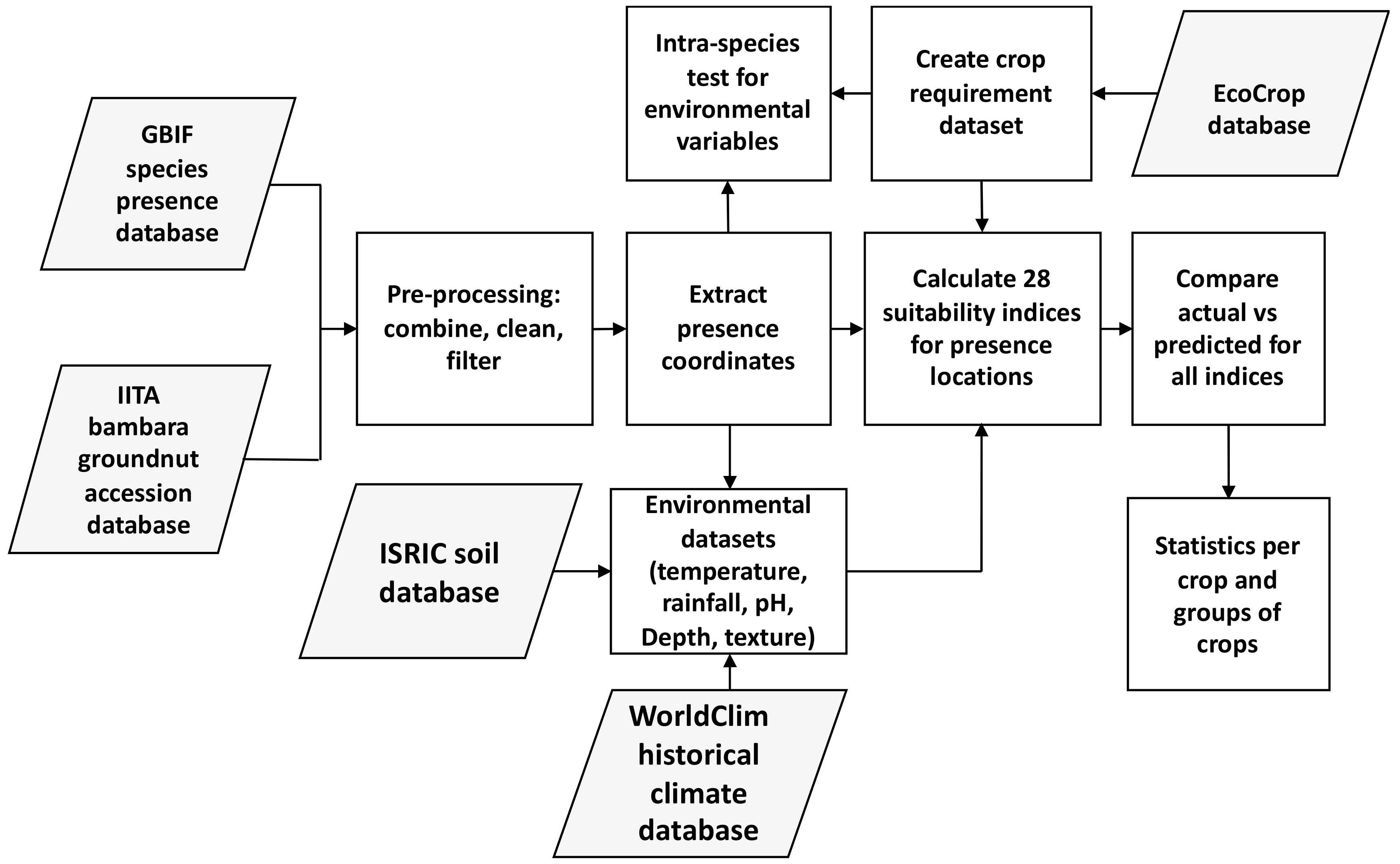
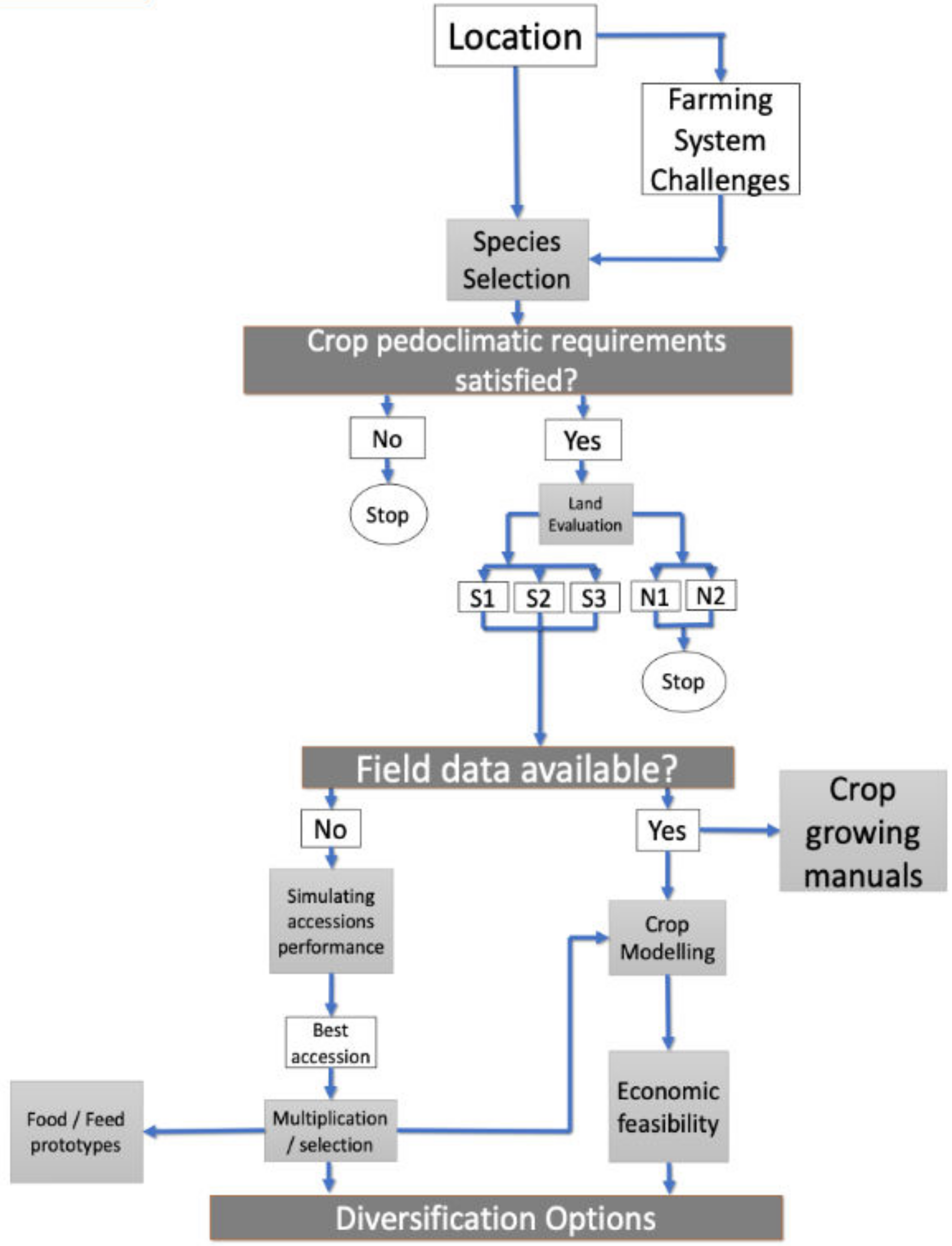
2. Materials and Methods

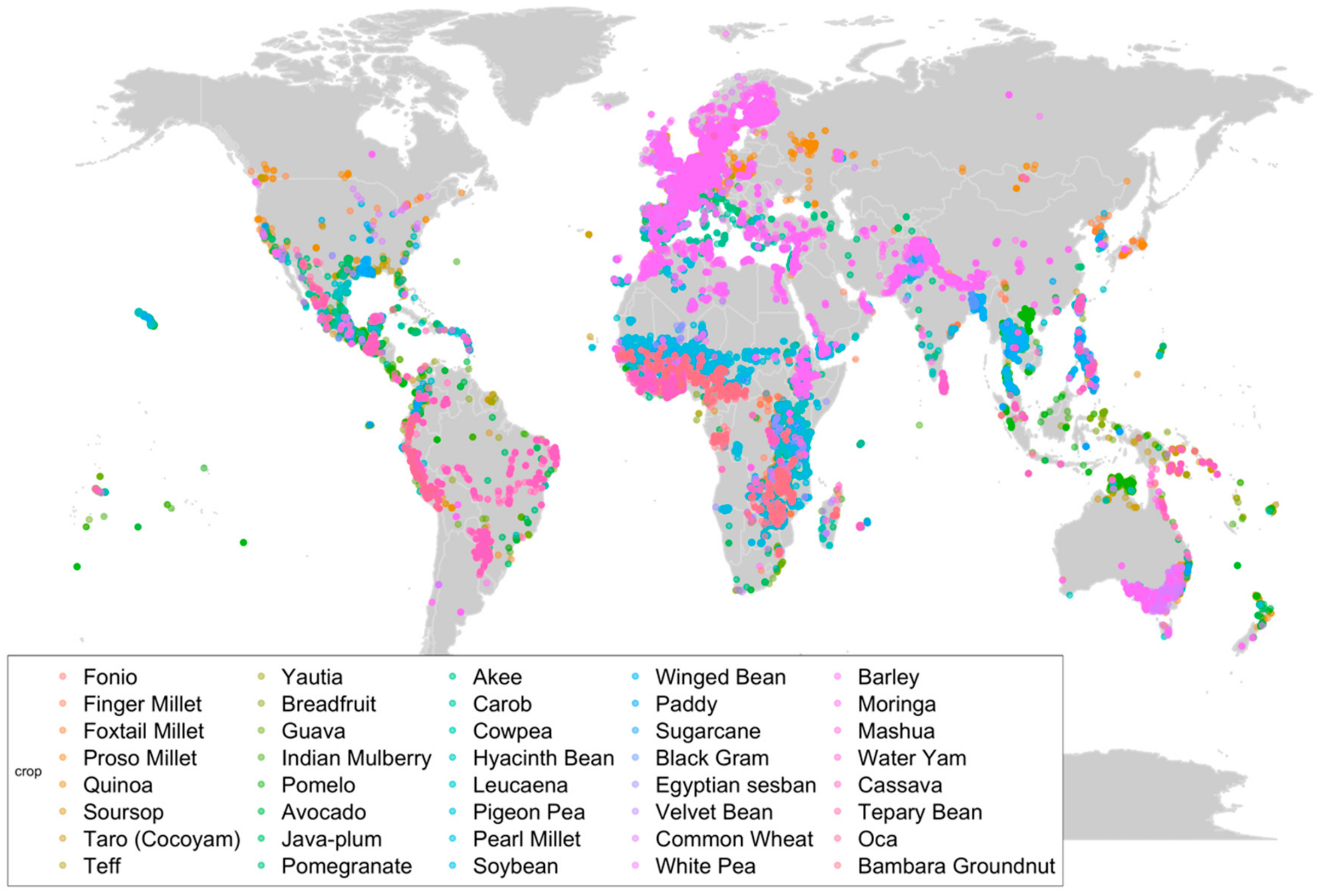
Figure 1 summarises the employed methodology and shows the sources of data and processing steps used to derive the final results.

2.1. Data

Species occurrence data for 40 crops representing both major and underutilised crops were obtained from the GBIF (Global Biodiversity Information Facility) database [26]. The chosen species represented a combination of crop types including cereals, legumes, vegetables, tubers/roots, and fruits (

Table 1. List of crops categorized into crop types.

Cereals, Pseudo-Cereals, and Grasses	Legumes and Vegetables
Barley—Hordeum vulgare L. Common Wheat—Triticum aestivum L. Finger Millet—Eleusine coracana Gaertn. Fonio—Digitaria exilis Stapf Foxtail Millet—Setaria italica P.Beauv. Paddy—Oryza sativa L. Pearl Millet—Pennisetum glaucum (L.) R.Br. Proso Millet—Panicum miliaceum L. Quinoa—Chenopodium quinoa Willd. Sugarcane—Saccharum officinarum L. Teff—Eragrostis tef (Zuccagni) Trotter	Black Gram—Vigna mungo (L.) Hepper Bambara groundnut—Vigna subterranea (L.) Verdc. Cowpea—Vigna unguiculata subsp. unguiculata Egyptian sesban—Sesbania sesban Merr. Hyacinth Bean—Lablab purpureus (L.) Sweet Leucaena—Leucaena leucocephala (Lam.) de Wit Pigeon pea—Cajanus cajan (L.) Millsp. Soybean—Glycine max (L.) Merr. Velvet Bean—Mucuna pruriens (L.) DC. White Pea—Lathyrus sativus L. Winged Bean—Psophocarpus tetragonolobus DC. Tepary Bean—Phaseolus acutifolius A.Gray Moringa—Moringa oleifera Lam
Tuber/Roots	Fruits
Taro (Cocoyam)—Colocasia esculenta (L.) Schott Yautia—Xanthosoma sagittifolium (L.) Schott Mashua—Tropaeolum tuberosum Ruiz & Pav Water Yam—Dioscorea alata L Cassava—Manihot esculenta Crantz Oca—Oxalis tuberosa Molina	Akee—Blighia sapida Kon. Avocado—Persea americana Mill. Breadfruit—Artocarpus altilis (Parkinson) Fosberg Carob—Ceratonia siliqua L. Guava—Psidium guajava L. Indian Mulberry—Morinda citrifolia L. Java-plum—Syzygium cumini (L.) Skeels Pomegranate—Punica granatum L. Pomelo—Citrus maxima (Burm.) Merr. Soursop—Annona muricata L.

).

The geographical extent of the analysis was global with crop presence data scattered over the globe (Figure 2).

Agroecological requirements for individual crops were extracted from FAO EcoCrop [25] (Appendix A). To demonstrate the ability of these environmental thresholds to encompass genetic variation, the same methodology was used to assess more than 1000 accessions of bambara groundnut (Vigna subterranea (L.) Verdc.) obtained from IITA (International Institute of Tropical Agriculture) [27].

Climate data were acquired from the WorldClim interpolated global climate dataset at 1 km spatial resolution [28]. Soil data were acquired from the SoilGrids global dataset that provides gridded data based on a database of 150,000 soil profiles and physically based covariates including geomorphological data and global datasets of satellite images at 250 m spatial resolution [29]. Soil chemical and structural properties known to affect crop yield were identified. Soil texture was defined by three binary variables describing suboptimal and optimal conditions from “light” to “heavy” texture classes. This form of data specification was adopted due to the format of the FAO EcoCrop database that describes texture using qualitative keywords such as “light”, “medium”, and “heavy” rather than quantitative variables. This information was used to prespecify soil texture in the form of % sand and % clay using known soil texture classifications [30]. An expert-defined optimal soil depth based on the EcoCrop data was used to determine the effective depth for aggregating soil properties (pH, % sand, and % clay) within the standard SoilGrids depth intervals using numerical integration methods. For each coordinate, soil and climate data were extracted from the soil and climate layers and harmonised for use in calculating suitability indices.

2.2. Computational Aspects

All data processing and analysis used open source software. Species presence and accession data were manually downloaded from the GBIF and IITA databases and stored in Comma-separated values (CSV) format. A script was developed in R statistical language version 3 [31] to automatically extract scientific names from each record. This script excluded records without coordinates and preserved only those records in the GBIF dataset that were real observations in the field (about 95% of total observations) [32]. Another automatic script was developed to extract records of climate (temperature and rainfall) and soil (pH, % sand, % clay, and depth to bedrock) from worldClim and International Soil Reference and Information Centre (ISRIC) data layers. The scripts were designed to run on a central server to facilitate data extraction for a large number of coordinates.

Another R script was written to calculate both individual and combined suitability indices for each occurrence record and to aggregate the results for analysis and to display as tables and figures. All R scripts were run on a Macintosh computer (MacOS 11); the run time for calculating the indices and for preparing the results was about 15 hours. All scripts and data are available at https://github.com/geoej/LEFAD [33].

2.3. Deriving the Indices

Calculation starts with determining a temperature suitability index for all possible growing seasons starting from January and then proceeding monthly. The index specifies suitability for optimal and suboptimal conditions for each month, $T_{mi}$:

$$T_{mi}=\left\{\begin{array}{cc}0\hfill & \hfill T_{a_i}<T_{Amin}\\ \frac{T_{a_i}-T_{Amin}}{T_{Omin}-T_{Amin}}\times 100\hfill & \hfill T_{Amin}< T_{a_i}<T_{Omin}\\ 100\hfill & \hfill T_{Omin}<T_{a_i}<T_{Omax}\\ \left(1-\frac{T_{a_i}-T_{Omax}}{T_{Amax}-T_{Omax}}\right)\times 100\hfill & \hfill \hspace{1em}\hspace{1em}{T}_{Omax}<T_{a_i}<T_{Amax}\\ 0\hfill & \hfill T_{a_i}>T_{Amax}\end{array}\right\}$$

(1)

where $T_{a_i}$ is the average monthly temperature for the location i, $T_{Amin}$ and $T_{Amax}$ are the marginal or absolute temperature averages for a species to survive, and $T_{Omin}$ and $T_{Omax}$ are the optimal minimum and maximum temperature averages for the species to grow and produce yield based on the original EcoCrop model [18]. This suitability index distinguishes suboptimal from optimal conditions by assigning a lower index to temperature ranges that might result in plant germination but are generally less hospitable for sustained growth and may lead to yield loss.

To reduce the computational burden, only average temperature as an indicator of thermal requirement was used. This allows the algorithm to run once instead of twice for $T_{imin}$ and $T_{imax}$ as proposed by Ramirez-Villegas et al. [15].

Next, the algorithm calculates the length of growing season by determining the growing days from sowing/transplanting to the end of the growing season or next harvest (for perennial crops). For any location, the seasonal temperature suitability for a crop is the minimum of all monthly indices (n) that fall within season s:

$$T{S}_{s_i}=\min \left(T_{m{1}_i}, T_{m{2}_i},\dots ,T_{m{n}_i}\right)$$

(2)

where $T{S}_{s_i}$ is total temperature suitability for season s at location i. The same calculation is repeated for rainfall suitability, except that rainfall is aggregated for all months within all possible seasons (n) in the calendar year first:

$$R_{s_i}=\mathrm{sum}\left(R_{m{1}_i}, R_{m{2}_i},\dots ,R_{m{n}_i}\right)$$

(3)

$$R{S}_{s_i}=\left\{\begin{array}{cc}0\hfill & \hfill R_{s_i}<R_{Amin}\\ \frac{R_{s_i}-R_{Amin}}{R_{Omin}-R_{Amin}}\times 100\hfill & \hfill R_{Amin}<R_{s_i}<R_{Omin}\\ 100\hfill & \hfill R_{Omin}<R_{s_i}<R_{Omax}\\ \left(1-\frac{R_{s_i}-R_{Omax}}{R_{Amax}-R_{Omax}} \right)\times 100\hfill & \hfill R_{Omax}<R_{s_i}<R_{Amax}\\ 0\hfill & \hfill R_{s_i}>R_{Amax}\end{array}\right\}$$

(4)

where $R_{s_i}$ is the sum of rainfalls ($R_{mi}$) for season s at location i and $R_{Amin}$, $R_{Omin}$, $R_{Omax}$, and $R_{Amax}$ are the rainfall requirements for marginal and optimal conditions in millimetres/season based on data provided by the FAO EcoCrop database.

For optimal depth suitability, $D{S}_i$, a binary system was developed:

$$D{S}_i=\left\{\begin{array}{cc}100\hfill & \hfill C_{od}=low AND 0_{cm}<Dt{B}_i<{50}_{cm}\\ 100\hfill & \hfill C_{od}=medium AND {50}_{cm}<Dt{B}_i<{100}_{cm}\\ 100\hfill & \hfill C_{od}=deep AND {100}_{cm}<Dt{B}_i<{200}_{cm}\\ \hspace{1em}0\hfill & \hfill other conditions\hspace{1em}\end{array}\right\}$$

(5)

where $C_{od}$ is the optimal depth of soil the crop requires to establish its rooting system and $Dt{B}_i$ is depth to bedrock at location i. The rooting system of plants can often change in response to environment, but due to lack of information describing that relationship, the cutoffs in Equation (5) were used to simulate the impact of soil depth on plant growth.

A pH suitability index was calculated by defining optimal and suboptimal conditions for plant growth:

$$pH{S}_i=\left\{\begin{array}{cc}0\hfill & \hfill p{H}_i<p{H}_{Amin}\\ \frac{p{H}_i-p{H}_{Amin}}{p{H}_{Omin}-p{H}_{Amin}}\times 100\hfill & \hfill p{H}_{Amin}<p{H}_i<p{H}_{Omin}\\ 100\hfill & \hfill p{H}_{Omin}<p{H}_i<p{H}_{Omax}\\ \left(1-\frac{p{H}_i-p{H}_{Omax}}{p{H}_{Amax}-p{H}_{Omax}}\right)\times 100\hfill & \hfill p{H}_{Omax}<p{H}_{is}<p{H}_{Amax}\\ 0\hfill & \hfill p{H}_{is}>p{H}_{Amax}\end{array}\right\}$$

(6)

The pH value for any location, i, is dependent on the optimal soil depth and was aggregated for three effective depths: low (0–50 cm), medium (0–150 cm), and deep (0-<200 cm) with the trapezoidal rule used to integrate soil data at different depths [29].

$${{\displaystyle \int }}_a^{b}f\left(x\right)dx \approx \frac{1}{\left(b-a\right)}\frac{1}{2}{{\displaystyle \sum }}_{k=1}^{N-1}\left(x_{k+1}-x_k\right)\left(f\left(x_k\right)+f\left(x_{k+1}\right)\right)$$

(7)

where N is the number of standard depths that can fit into the optimal soil depth for a crop for any specific soil property (i.e., pH, % sand, % clay, etc.), $f(x_k)$ is the value of soil property at depth k, and a and b are target depths in centimetres.

The optimal soil texture requirements (light, medium, and heavy) were converted to % sand and % clay based on the particle-size classification method for linking texture classes to sand and clay percentages by United States Department of Agriculture (USDA) soil survey manual [30]. The sand and clay values were “depth standardised” as for pH. The final rule for deriving the texture index was

$$TXT{S}_i=\left\{\begin{array}{cc}100\hfill & C_{ot}=heavy AND SN{D}_i<65\\ 100\hfill & \hspace{1em}{C}_{ot}=medium AND SN{D}_i<52 \mathrm{OR} CL{Y}_i<27\\ 100\hfill & C_{ot}=light AND CL{Y}_i<15\\ 25& \hspace{1em}\hspace{1em}\hspace{1em}\hspace{1em}\hspace{1em}\hspace{1em}\hspace{1em}\hspace{1em}else\end{array}\right\}$$

(8)

where $C_{ot}$ is the optimal soil texture required for a given crop. Soil texture was considered as a function of $SN{D}_i$ and $CL{Y}_i$ variables which are the relative presences of sand and clay particles. To reduce the computational burden, a simple set of rules were selected to reflect the soil texture and its relation to soil structure as an important driver of soil quality [4]. For example, if a crop grows optimally in “heavy-textured” soils, then a soil containing more than 65% sand particles will be inhospitable for that crop. Likewise, a clay content >15% poses a serious growth limitation on crops that prefer “light-textured” soils. Soils that contain <52% sand and <27% clay were considered loamy and suitable for crops that require “medium-textured” soils. These limits were chosen based on the USDA soil survey manual [30,34] that relates soil particle-size percentages to textural classes (see Appendix B).

Table 2. Individual as well as combined suitability (interactions) indices and their mathematical formula.

Index	Formula
Thermal	$T{S}_{is}$
Rainfall	$R{S}_{is}$
pH	$pH{S}_i$
Depth	$D{S}_i$
Texture	$TXT{S}_i$
Thermal × Rainfall	$R{S}_{is}\times T{S}_{is}$
Average (Thermal, Rainfall)	$\left(R{S}_{is}\times T{S}_{is}\right)/2$
pH × Texture × Depth	$pH{S}_i\times D{S}_i\times TXT{S}_i$
Average (pH, Texture, Depth)	$\left(pH{S}_i+D{S}_i+TXT{S}_i\right)/3$
Average (0.6 × pH, 0.2 × Texture, 0.2 × Depth)	$\left(0.6\times pH{S}_i+0.2\times D{S}_i+0.2\times TXT{S}_i\right)/3$
Thermal × Rainfall × pH × Texture × Depth	$R{S}_{is}\times T{S}_{is}\times pH{S}_i\times D{S}_i\times TXT{S}_i$
Average ((Thermal × Rainfall), (pH × Texture × Depth))	$((R{S}_{is}\times T{S}_{is})+\left(pH{S}_i\times D{S}_i\times TXT{S}_i\right))/2$
(Thermal × Rainfall) × Average (pH, Texture, Depth)	$(R{S}_{is}\times T{S}_{is})\times \left(pH{S}_i+D{S}_i+TXT{S}_i\right)/3$
Average ((Thermal × Rainfall), Average (pH, Texture, Depth))	$\left((R{S}_{is}\times T{S}_{is}\right)+\left(pH{S}_i+D{S}_i+TXT{S}_i\right)/3)/2$
(Thermal × Rainfall) × Average (0.6 × pH, 0.2 × Texture, 0.2 × Depth)	$\left(R{S}_{is}\times T{S}_{is}\right)\times \left(0.6\times pH{S}_i+0.2\times D{S}_i+0.2\times TXT{S}_i\right)$
Average ((Thermal × Rainfall), Average (0.6 × pH, 0.2 × Texture, 0.2 × Depth))	$\left((R{S}_{is}\times T{S}_{is}\right)+\left(0.6\times pH{S}_i+0.2\times D{S}_i+0.2\times TXT{S}_i\right)/3)/2$
Average (Thermal, Rainfall) × pH × Texture × Depth	$\left(\left(R{S}_{is}+T{S}_{is}\right)/2\right)\times \left(pH{S}_i\times D{S}_i\times TXT{S}_i\right)$
Average ((Thermal, Rainfall), (pH × Texture × Depth))	$\left(\left(\frac{\left(R{S}_{is}+T{S}_{is}\right)}{2}\right)+\left(pH{S}_i\times D{S}_i\times TXT{S}_i\right)\right)/2$
Average (Thermal, Rainfall) × Average (pH, Texture, Depth)	$\left(\frac{\left(R{S}_{is}+T{S}_{is}\right)}{2}\right)\times \left(pH{S}_i+D{S}_i+TXT{S}_i\right)/3$
Average ((Thermal, Rainfall), Average (pH, Texture, Depth))	$\left(\left(\frac{\left(R{S}_{is}+T{S}_{is}\right)}{2}\right)+\left(pH{S}_i+D{S}_i+TXT{S}_i\right)/3\right)/2$
Average (Thermal, Rainfall) × Average (0.6 × pH, 0.2 × Texture, 0.2 × Depth)	$\left(\left(\frac{\left(R{S}_{is}+T{S}_{is}\right)}{2}\right)\times \left(0.6\times pH{S}_i+0.2\times D{S}_i+0.2\times TXT{S}_i\right)\right)$
Average ((Thermal, Rainfall), Average (0.6 × pH, 0.2 × Texture, 0.2 × Depth))	$\left(\left(\frac{\left(R{S}_{is}+T{S}_{is}\right)}{2}\right)+\left(0.6\times pH{S}_i+0.2\times D{S}_i+0.2\times TXT{S}_i\right)\right)/2$
Thermal × pH × Texture × Depth	$T{S}_{is}\times pH{S}_i\times D{S}_i\times TXT{S}_i$
Average (Thermal, (pH × Texture × Depth))	$\left(T{S}_{is}+\left(pH{S}_i\times D{S}_i\times TXT{S}_i\right)\right)/2$
Thermal × Average (pH, Texture, Depth)	$T{S}_{is}\times \left(\frac{\left(pH{S}_i+D{S}_i+TXT{S}_i\right)}{3}\right)$
Average (Thermal, Average (pH, Texture, Depth))	$(T{S}_{is}+\left(\left(pH{S}_i+D{S}_i+TXT{S}_i\right)/3\right)/2$
Thermal × Average (0.6 × pH, 0.2 × Texture, 0.2 × Depth)	$(T{S}_{is}+\left(0.6\times pH{S}_i+0.2\times D{S}_i+0.2\times TXT{S}_i\right)$
Average (Thermal, Average (0.6 × pH, 0.2 × Texture, 0.2 × Depth))	$(T{S}_{is}+\left(0.6\times pH{S}_i+0.2\times D{S}_i+0.2\times TXT{S}_i\right)/2$

shows a range of final suitability indices for a season s, ($C{S}_{is}$) and the maximum of all possible yearly seasons (n) will determine final suitability ($C{S}_i=\max \left(C{S}_{i1}, C{S}_{i2}, \dots ,C{S}_{in}\right)$).

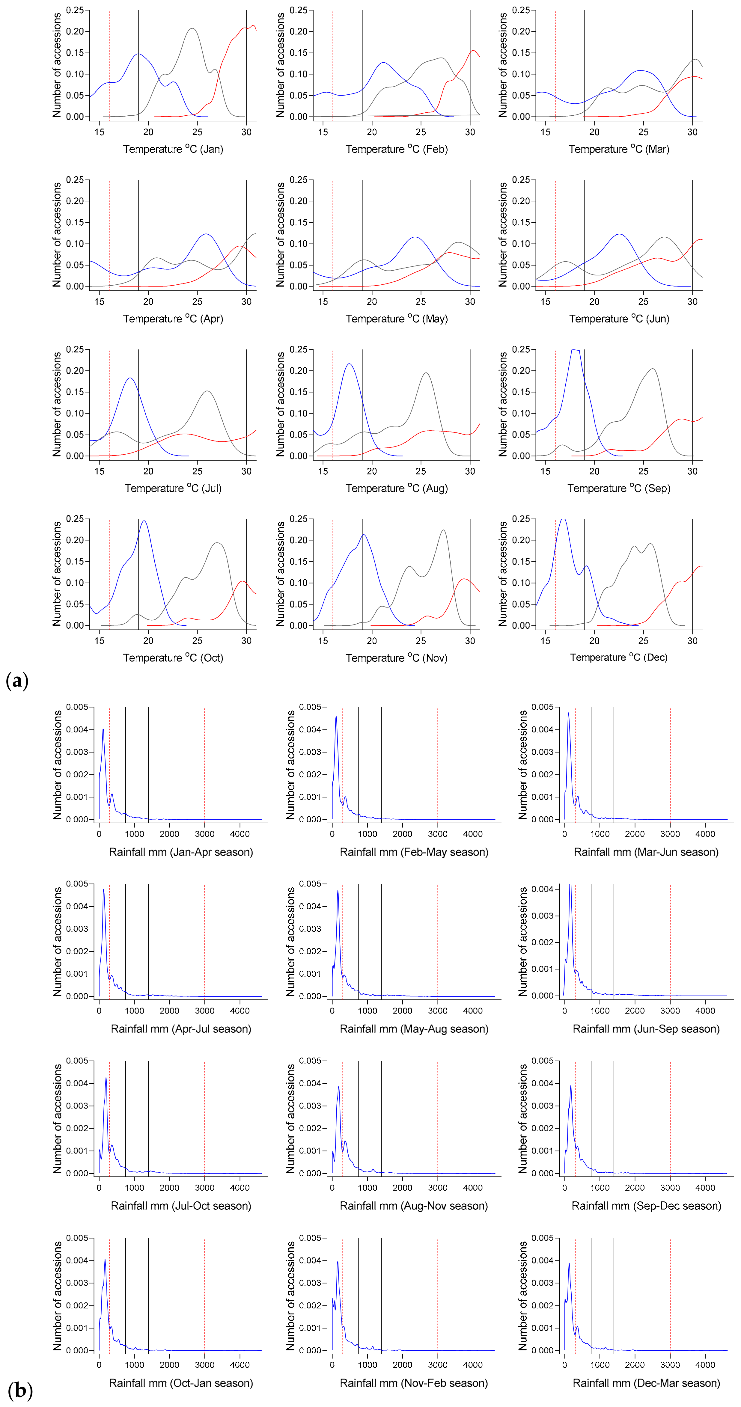
2.4. Accounting for Intraspecies Variation

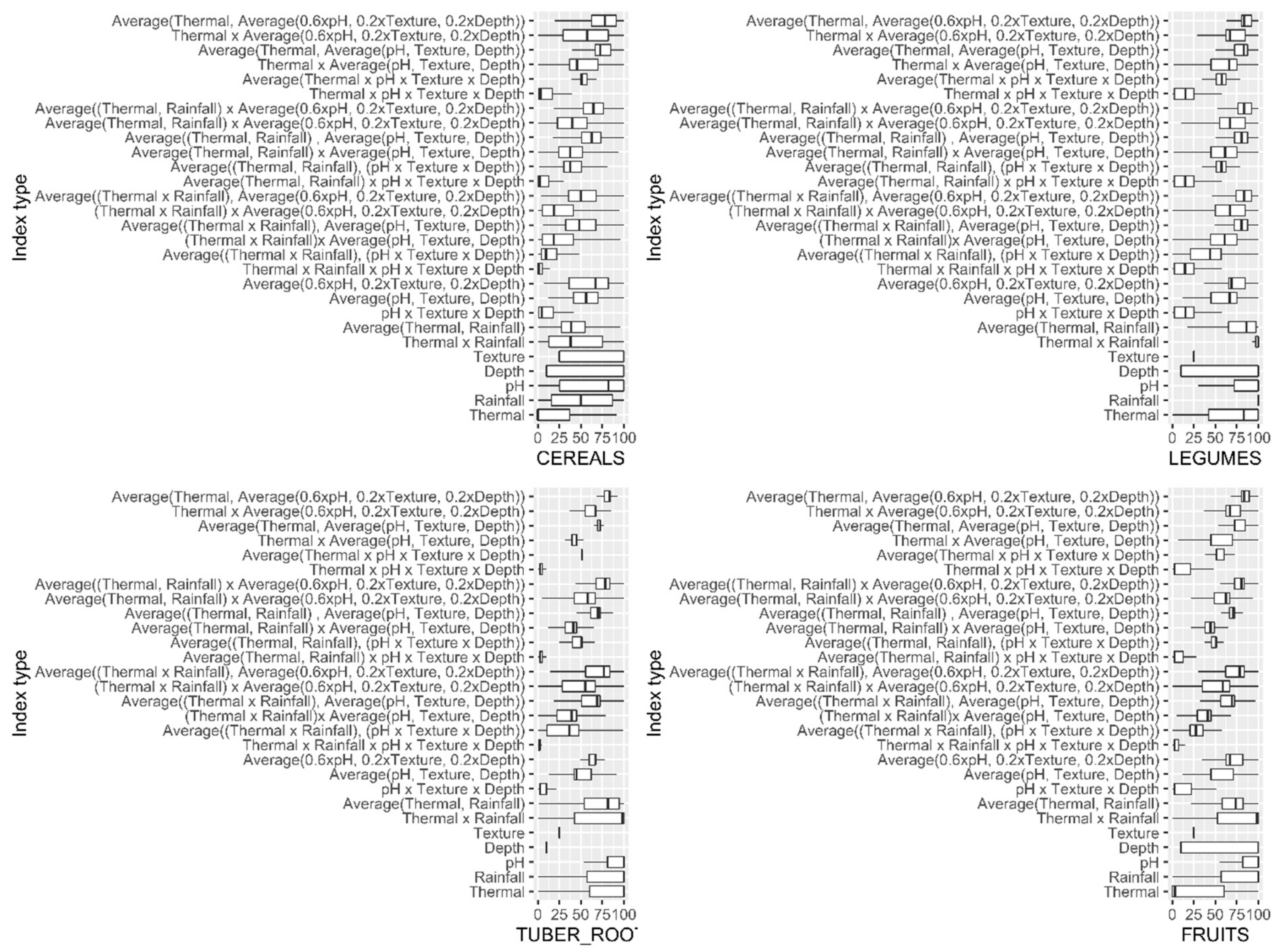
To test the ability of the expert-defined species threshold data to describe within species variation, an assessment was undertaken using multiple cultivars of bambara groundnut (Vigna subterranea (L.) Verdc.) as an exemplar underutilised crop [1]. Soil and climate data were extracted based on accession locations [27] and checked for consistency, and kernel density plots (frequency per 0.1 increment) of their pedoclimatic distribution were created. According to the EcoCrop database, the optimal soil texture for bambara groundnut is “light”. Therefore, to create quantitative thresholds, soils with clay particles of 10%–20% (“sand” and “loamy sand” texture classes) were considered optimal [30].

3. Results

Of the 28 indices used to calculate suitability at the locations where crops were observed, the pH suitability index and the combined weighted average of thermal suitability index with all soil indices (numbers 1 and 2,

Table 3. A correlation analysis of mean value of “predicted presence” versus “actual presence” of all crops in Table 1 and for individual indices and their interactions.

No	Final Suitability Index	Mean	SD	Median	Min.	Max.
1	pH	85	14	89	41	99
2	Average (Thermal, Average (0.6 × pH, 0.2 × Texture, 0.2 × Depth))	82	7	82	58	92
3	Average (Thermal, Average (pH, Texture, Depth))	77	8	75	53	88
4	Average ((Thermal, Rainfall) × Average (0.6 × pH, 0.2 × Texture, 0.2 × Depth))	74	10	79	53	91
5	Average ((Thermal, Rainfall), Average (pH, Texture, Depth))	69	10	70	47	87
6	Average (0.6 × pH, 0.2 × Texture, 0.2 × Depth)	69	9	70	43	85
7	Rainfall	66	30	80	1	98
8	Average ((Thermal × Rainfall), Average (0.6 × pH, 0.2 × Texture, 0.2 × Depth))	66	17	73	29	91
9	Thermal × Average (0.6 × pH, 0.2 × Texture, 0.2 × Depth)	65	11	65	33	84
10	Thermal × Rainfall	63	31	76	1	98
11	Average (Thermal, Rainfall)	61	22	66	13	92
12	Average ((Thermal × Rainfall), Average (pH, Texture, Depth))	61	16	65	22	86
13	Average (pH, Texture, Depth)	59	12	59	32	77
14	Average (Thermal, Rainfall) × Average (0.6 × pH, 0.2 × Texture, 0.2 × Depth)	56	15	61	28	83
15	Thermal × Average (pH, Texture, Depth)	55	14	51	28	76
16	Average (Thermal × pH × Texture × Depth)	55	8	52	31	72
17	Thermal	53	32	62	0	99
18	Depth	52	41	30	10	100
19	Average ((Thermal, Rainfall), (pH × Texture × Depth))	47	10	49	24	62
20	Average (Thermal, Rainfall) × Average (pH, Texture, Depth)	47	14	43	22	74
21	(Thermal × Rainfall) × Average (0.6 × pH, 0.2 × Texture, 0.2 × Depth)	44	23	53	1	83
22	Texture	39	16	29	26	82
23	(Thermal × Rainfall) × Average (pH, Texture, Depth)	37	20	39	0	73
24	Average ((Thermal × Rainfall), (pH × Texture × Depth))	26	15	23	2	53
25	pH × Texture × Depth	14	11	12	2	45
26	Thermal × pH × Texture × Depth	13	11	8	2	45
27	Average (Thermal, Rainfall) × pH × Texture × Depth	11	9	8	2	26
28	Thermal × Rainfall × pH × Texture × Depth	9	8	5	0	25

) estimated the presence for all crops better than 80%. Although the pH index best predicted the presence in terms of overall mean, the interaction index (No. 2) had the lowest standard deviation among all indices. The other soil indices did not perform well compared to the climate indices. Giving more weight to pH suitability had a generally positive impact on those indices that averaged all the variables.

Figure 3 shows a boxplot comparison of the indices for the groups of crops. Again, the best result in terms of mean and SD was for indices at the top of the list for all groups of crops with the exception of cereals that were more variable (reflected in the long tail of the boxplot). The results show that, despite poor performance, the soil-weighted averages had the lowest variation, suggesting that all available soil information could still be used advantageously in the suitability assessments.

Intraspecies Test

The majority of locations where bambara groundnut accessions were collected fell between the solid lines, representing the optimal soil pH conditions based on expert knowledge provided by the FAO EcoCrop database (Figure 4). Some locations had soils containing more than 20% clay—values which are suboptimal for the growth of bambara groundnut due to poor drainage/aeration issues [35]. For depth to bedrock, the majority of locations where accessions were collected had a depth >175 cm.

Figure 5 shows the same pattern for monthly average temperature as that shown for pH. The grey curve, which represents average temperature for collected accession locations, is within the optimal temperature range for the majority of calendar months. The cumulative seasonal rainfall for all calendar seasons showed very low precipitation for all locations where accessions were collected, suggesting that the majority of accessions might have been collected from irrigated fields. Therefore, the amount of required precipitation alone was not a suitable criterion for determining suitability as information about management practices of the accessions are largely unknown.

4. Discussion

4.1. Intraspecies Variation

Analysis of the accession data for bambara groundnut showed that the species threshold information could correctly represent intraspecies variation. Although some locations fell outside the ranges defined by expert knowledge, it was evident that the within species variation of bambara groundnut could be reliably represented by these expert-defined thresholds when compared with the known distribution of the crop as compiled from Food and Agriculture Organization Corporate Statistical Database (FAOSTAT) [36]. Threshold values can also be validated using statistical methods. For example, Ramirez-Villegas, Jarvis, and Läderach [15] used simple population statistics to derive these parameters for grain sorghum. Nevertheless, this requires extensive presence/accession data to be available for all crops.

Georeferenced accession data can be useful in determining ecological niches at the sub-taxa level and can be used to select specific genotypes that can perform well at a particular location [37]. The method proposed here could also potentially benefit breeding programmes for desirable traits such as drought and heat tolerance by selecting accessions that are collected at places with high temperature and low precipitation (Figure 5).

4.2. Combined Suitability Assessment

Many Ecocrop-based models consider crop suitability only as a function of climate information [14,15,21]. In this work, pH was chosen as representative of soil chemical properties that can affect nutrient availability, with texture and depth to bedrock as representatives of soil physical properties. Overall, the results (Table 3) showed that local climate information alone is not a good indicator of suitability. Furthermore, within major crop groups, the climate-only indices had the highest variability, particularly for the indices that used aggregated seasonal rain; this is evident in the bottom half of the group boxplots (Figure 3). The main reason for this could be that information about the cropping systems are not exhaustively documented by the gene banks [38], and therefore, distinguishing between rainfed, irrigated, and other management practices for all locations is not possible.

Using soil pH as an indicator of crop suitability resulted in an overall median accuracy of estimation of 89%. However, a suitability index that took account of the interaction between thermal requirements with weighted averages of all soil properties produced the lowest standard deviation (Table 3 and Figure 3). This confirms improvements reported by Piikki et al. [19] for common bean (Phaseolus vulgaris L.) in Tanzania using soil organic matter. Also, Velazco et al. [20] reported the same results using similar edaphic variables. However, their study focused on habitat prediction only for trees, shrubs, herbs, and palm plants at a continental extent. Comparison between the pH-only index and the more complex weighted average interaction index (rows number 1 and 2, Table 3) suggests that adding more local information with a reasonable amount of accuracy (see Section 4.4) reduces variation in the final results. Setting aside the costs of soil remediation and unless for specific acid or alkali tolerant crops, pH-related issues can be remedied with proper management strategies. Therefore, it might be argued that pH alone is not a suitable indicator for crop suitability because many crops can grow in a range of soils provided pH issues can be remedied. Therefore, the use of the more complex interaction index is a better reasonable solution to delineate local options.

4.3. Combining with Traditional Land System Models

The index based on quantitative and qualitative environmental thresholds introduced here can be combined with traditional land models such as the FAO land evaluation system [5] to classify suitability based on designated suitability classes (S1: 80–100, S2: 60–80, and S3: 40–60; N1:20–40 and N2: 0–20), after combining the index with the local land-use units (e.g., agriculture land, etc.) using known land use classification methods [39]. This can provide an initial estimate of crop suitability for a large number of crops; for example, there are data for more than 2500 species in the FAO EcoCrop inventory. Moreover, suitability of cropping systems such as monocropping, intercropping, and mixed-cropping for both arable and marginal lands [11] can be assessed by combining crops from different groups that have the same index at a particular location. This method can also be used to delineate adaptation strategies for climate change in agroecological zones [40] where change in season length and occurrence or intensity of precipitation have affected current practices. More robust diversification strategies can be investigated by combining other important factors including germplasm availability and socioeconomic factors such as desired income level for farmers by delineating distance to market [41] and crop macro- and micronutrients to alleviate nutrition deficiency.

Bouma et al. [42] defined a classification system for land-use modelling approaches (empirical, mechanical, qualitative, and quantitative) based on available soil data at different spatial scales (global, continental, regional, watershed, catena/farm/field/plot, soil horizon and structure, and molecular interaction) and available soil/land knowledge levels (1 = user, 2 = expert, 3 = semiquantitative, and 4 and 5 = different levels of quantitative knowledge) when dealing with land-use questions. This is a useful schema for determining what type of approach is required for dealing with different users with different levels of knowledge at different scales. The approach described in this article is at level two in terms of “crop knowledge” (agrobiodiversity knowledge) and at four in terms of “soil and climate knowledge”. However, the output “crop suitability information” still remains at level two (expert/estimated knowledge), since information such as “bambara groundnut is a moderately suitable crop for this field” is insufficient for farmers but can be enough for a regional planner looking for possibilities beyond current practices at the mesoscale (regional or national).

Other soil variables such as organic content, salinity, and bulk density can be added to this methodology, provided reliable data are available. This will require the development of analytical methods that can convert “qualitative” information such as “soil fertility level = medium”, “saline tolerance = low”, etc. used in describing favourable conditions for a crop, into quantitative scales such as organic carbon content (g/kg), cation exchange capacity (cmol + /kg), and volumetric % of coarse fragment in soil.

Figure 6 shows a decision framework for global diversification projects in which selection can be initiated for a location following a baseline study of the local farming systems to ascertain local priorities for crop diversification. The results of shortlisting using pedoclimatic analysis can be combined with land system models to elevate the information to level 3 (semiquantitative knowledge) in Bouma’s classification. Combining the results with crop models will improve the output to levels 4 and 5 (quantitative knowledge) with the inclusion of other data types such as solar radiation, crop water and nutrient use efficiency, etc. Such quantitative modelling efforts can be carried out with either experimental data from known crop genotypes/varieties or landraces [43] or with simulations of suitability for accessions collected in similar pedoclimatic conditions using globally available datasets [37,44]. Finally putting all of these insights together in open access software tools can help with rapid delineation of alternative cropping options.

4.4. Limitations in Method, Data, and Computational Aspects

The two datasets used for species occurrence data for crop groups (GBIF) and bambara groundnut accession (IITA) contained data of different quality. For instance, although GBIF has introduced the concept of coordinate uncertainty in its database, IITA does not include that information. Also, coordinates are documented without adequate metadata (in the case of numerical coordinates, that means latitudes and longitudes are recorded without additional decimal points). Also, both of these databases do not usually record details of plant and environmental interactions such as the type of cropping system from which the presence/accessions were observed/acquired [38].

As Hengl et al. [29] state, predicted soil variables in the SoilGrids dataset are of different levels of certainty, particularly for areas where soil profile data are scarce. The uncertainty level is also different among predicted soil properties. For example, although the predicted pH values had an overall R-square of 83.4% and root mean square error (RMSE) of 0.5, the depth to bedrock model could only explain close to half of the variation (R-square of 54.0%). This issue is manifested in Figure 4 for depth to bedrock, where the expert-defined thresholds and soil depth where the accessions were collected do not agree.

The global cross validation for the climate dataset using the weather station data showed high accuracy for temperature with a correlation coefficient of 0.99 and RMSE of 1.1 [28]. However, the model accuracy was low for predicted precipitation (RMSE of 49.5) due to lack of local weather station data or poor model specification. This confirms the findings here that the amount of reported precipitation at a location may not be a good indicator of suitability as it is possible to grow a crop economically and productively with irrigation [45]. Therefore, the present analysis should firstly be restricted to rain-fed systems.

5. Conclusions

Assessing potential of land for crop diversification using neglected and underutilised crop species at a specific location requires a practical approach that takes advantage of available data and knowledge. In this research, we used quantitative (temperature, rainfall, soil pH, and season length) and qualitative (optimal soil depth and soil texture) data to test a new method for estimating suitability of a wide range of crops. The analysis using more than 100,000 curated data representing crop presence showed that a suitability criterion based on soil pH and/or a moderated average suitability of temperature, pH, depth, and soil texture can predict the presence of a crop regardless of its type. The suitability index developed here distinguishes itself from traditional crop suitability evaluation methods in considering both climate and soil chemical and dynamic properties as well as potentially available local data. It can also be applied to a wide range of agricultural species, particularly those that are neglected and underutilised.

This method can be combined with traditional land evaluation systems and crop models to expand the range of cropping options in agricultural diversification projects. It can also be utilised in areas with shortage of resources such as water and where agrotechnology transfer is limited to propose diversification options. Although the output of this method is neither an estimate of crop biomass nor yield, it takes advantage of the availability of big environmental data and improvements in agricultural knowledge to improve our understanding of production systems involving minor crops. The same index can be used to compare many options at regional and local scales, where detailed data are available. The next logical step after suitability classification is to develop field trial programmes with local stakeholders that will lead to development of harmonised data inventories for the purpose of detailed yield estimations and crop insurance models such as those used for major crops.

References

1. Azam-Ali, S.N. Fitting underutilised crops within research-poor environments: Lessons and approaches. S. Afr. J. Plant Soil 2010, 27, 293–298. [Google Scholar] [CrossRef] [Green Version]
2. Mabhaudhi, T.; Modi, A.T. Sowing the seeds of knowledge on under-utilised crops: Indigenous crops - feature. Water Wheel 2016, 15, 40–41. [Google Scholar]
3. Dent, D.; Young, A. Soil Survey and Land Evaluation; E & FN Spon Allen & Unwin: London, UK, 1981; ISBN 978-0-419-15960-5. [Google Scholar]
4. Mueller, L.; Schindler, U.; Mirschel, W.; Shepherd, T.G.; Ball, B.C.; Helming, K.; Rogasik, J.; Eulenstein, F.; Wiggering, H. Assessing the productivity function of soils. A review. Agron. Sustain. Dev. 2010, 30, 601–614. [Google Scholar] [CrossRef]
5. FAO. Soil resources development and conservation service, land and water development division, FAO. A framework for land evaluation. In Soils Bulletin; Food and Agriculture Organisation of the United Nations: Rome, Italy, 1976; Volume 32. [Google Scholar]
6. Malone, B.P.; Kidd, D.B.; Minasny, B.; McBratney, A.B. Taking account of uncertainties in digital land suitability assessment. PeerJ 2015, 3, e1366. [Google Scholar] [CrossRef] [PubMed]
7. Manna, P.; Basile, A.; Bonfante, A.; De Mascellis, R.; Terribile, F. Comparative Land Evaluation approaches: An itinerary from FAO framework to simulation modelling. Geoderma 2009, 150, 367–378. [Google Scholar] [CrossRef]
8. Johnson, A.K.L.; Cramb, R.A. Development of a simulation based land evaluation system using crop modelling, expert systems and risk analysis. Soil Use Manag. 1991, 7, 239–246. [Google Scholar] [CrossRef]
9. Recatalá Boix, L.; Zinck, J.A. Land-Use Planning in the Chaco Plain (Burruyacú, Argentina). Part 1: Evaluating Land-Use Options to Support Crop Diversification in an Agricultural Frontier Area Using Physical Land Evaluation. Environ. Manag. 2008, 42, 1043–1063. [Google Scholar]
10. Qiu, F.; Chastain, B.; Zhou, Y.; Zhang, C.; Sridharan, H. Modeling land suitability/capability using fuzzy evaluation. GeoJournal 2014, 79, 167–182. [Google Scholar] [CrossRef]
11. Gerwin, W.; Repmann, F.; Galatsidas, S.; Vlachaki, D.; Gounaris, N.; Baumgarten, W.; Volkmann, C.; Keramitzis, D.; Kiourtsis, F.; Freese, D. Assessment and quantification of marginal lands for biomass production in Europe using soil-quality indicators. Soil 2018, 4, 267–290. [Google Scholar] [CrossRef] [Green Version]
12. Rötter, R.P.; Carter, T.R.; Olesen, J.E.; Porter, J.R. Crop–climate models need an overhaul. Nat. Clim. Chang. 2011, 1, 175–177. [Google Scholar]
13. Hoogenboom, G.; Pérez, C.L.; Rossiter, D.; Laake, P.V. Chapter 13 - Biophysical Agricultural Assessment and Management Models for Developing Countries. In Quantifying Sustainable Development; Hall, C.A.S., Perez, C.L., Leclerc, G., Eds.; Academic Press: San Diego, CA, USA, 2000; ISBN 978-0-12-318860-1. [Google Scholar]
14. Manners, R.; van Etten, J. Are agricultural researchers working on the right crops to enable food and nutrition security under future climates? Glob. Environ. Chang. 2018, 53, 182–194. [Google Scholar] [CrossRef]
15. Ramirez-Villegas, J.; Jarvis, A.; Läderach, P. Empirical approaches for assessing impacts of climate change on agriculture: The EcoCrop model and a case study with grain sorghum. Agric. For. Meteorol. 2013, 170, 67–78. [Google Scholar] [CrossRef]
16. Bonfante, A.; Monaco, E.; Alfieri, S.M.; De Lorenzi, F.; Manna, P.; Basile, A.; Bouma, J. Climate Change Effects on the Suitability of an Agricultural Area to Maize Cultivation. In Advances in Agronomy; Elsevier: Amsterdam, The Netherlands, 2015; Volume 133, pp. 33–69. ISBN 978-0-12-803052-3. [Google Scholar]
17. Zhao, C.; Liu, B.; Xiao, L.; Hoogenboom, G.; Boote, K.J.; Kassie, B.T.; Pavan, W.; Shelia, V.; Kim, K.S.; Hernandez-Ochoa, I.M.; et al. A SIMPLE crop model. Eur. J. Agron. 2019, 104, 97–106. [Google Scholar] [CrossRef]
18. Hijmans, R.J.; Guarino, L.; Cruz, M.; Rojas, E. Computer tools for spatial analysis of plant genetic resources data: 1. DIVA-GIS. Plant Genet. Resour. Newslett. 2001, 127, 15–19. [Google Scholar]
19. Piikki, K.; Winowiecki, L.; Vågen, T.-G.; Ramirez-Villegas, J.; Söderström, M. Improvement of spatial modelling of crop suitability using a new digital soil map of Tanzania. S. Afr. J. Plant Soil 2017, 34, 243–254. [Google Scholar] [CrossRef]
20. Velazco, S.J.E.; Galvão, F.; Villalobos, F.; De Marco Júnior, P. Using worldwide edaphic data to model plant species niches: An assessment at a continental extent. PLoS ONE 2017, 12, e0186025. [Google Scholar] [CrossRef] [Green Version]
21. Kim, H.; Hyun, S.W.; Hoogenboom, G.; Porter, C.H.; Kim, K.S. Fuzzy Union to Assess Climate Suitability of Annual Ryegrass (Lolium multiflorum), Alfalfa (Medicago sativa) and Sorghum (Sorghum bicolor). Sci. Rep. 2018, 8, 10220. [Google Scholar] [CrossRef]
22. Zabel, F.; Putzenlechner, B.; Mauser, W. Global Agricultural Land Resources – A High Resolution Suitability Evaluation and Its Perspectives until 2100 under Climate Change Conditions. PLoS ONE 2014, 9, e107522. [Google Scholar] [CrossRef] [Green Version]
23. Estes, L.D.; Bradley, B.A.; Beukes, H.; Hole, D.G.; Lau, M.; Oppenheimer, M.G.; Schulze, R.; Tadross, M.A.; Turner, W.R. Comparing mechanistic and empirical model projections of crop suitability and productivity: implications for ecological forecasting: Crop model intercomparison. Glob. Ecol. Biogeogr. 2013, 22, 1007–1018. [Google Scholar] [CrossRef]
24. Mabhaudhi, T.; Chimonyo, V.; Albert, M. Status of Underutilised Crops in South Africa: Opportunities for Developing Research Capacity. Sustainability 2017, 9, 1569. [Google Scholar] [CrossRef] [Green Version]
25. Land and Water Development Division of FAO. EcoCrop Database. Available online: http://ecocrop.fao.org/ecocrop/srv/en/about (accessed on 26 March 2019).
26. GBIF. Available online: https://www.gbif.org/ (accessed on 28 March 2019).
27. International Institute of Tropical Agriculture Bambara Groundnut Collection. Available online: http://my.iita.org/accession2/collection.jspx;jsessionid=A73728F581D906CDF43B9DC1D554090A?id=8 (accessed on 11 March 2019).
28. Fick, S.E.; Hijmans, R.J. WorldClim 2: new 1-km spatial resolution climate surfaces for global land areas: NEW CLIMATE SURFACES FOR GLOBAL LAND AREAS. Int. J. Climatol. 2017, 37, 4302–4315. [Google Scholar] [CrossRef]
29. Hengl, T.; Mendes de Jesus, J.; Heuvelink, G.B.M.; Ruiperez Gonzalez, M.; Kilibarda, M.; Blagotić, A.; Shangguan, W.; Wright, M.N.; Geng, X.; Bauer-Marschallinger, B.; et al. SoilGrids250m: Global gridded soil information based on machine learning. PLoS ONE 2017, 12, e0169748. [Google Scholar] [CrossRef] [PubMed] [Green Version]
30. USDA Soil Survey Manual; US Department of Agriculture: Washington, DC, USA, 1993.
31. R Core Team. R: A Language and Environment for Statistical Computing; R Core Team: Vienna, Austria,, 2013. [Google Scholar]
32. Global Biodiversity Information Facility. Available online: http://gbif.github.io/parsers/apidocs/org/gbif/api/vocabulary/BasisOfRecord.html (accessed on 26 March 2019).
33. Jahanshiri, E. geoej/LEFAD. A Land Evaluation Framework for Agricultural Diversification; Crops For the Future Research Centre: Semenyih, Malaysia, 2020. [Google Scholar] [CrossRef]
34. FAO Soil Texture Training Manual. Available online: http://www.fao.org/tempref/FI/CDrom/FAO_Training/FAO_Training/General/x6706e/x6706e06.htm (accessed on 20 March 2020).
35. Heller, J.; Begemann, F.; Mushonga, J. Bambara groundnut, Vigna subterranea (L.) Verdc. Promoting the Conservation and Use of Underutilized and Neglected Crops; International Plant Genetic Resources Institute: Gatersleben, Germany, 1997; ISBN 978-92-9043-299-9. [Google Scholar]
36. Monfreda, C.; Ramankutty, N.; Foley, J.A. Farming the planet: 2. Geographic distribution of crop areas, yields, physiological types, and net primary production in the year 2000: GLOBAL CROP AREAS AND YIELDS IN 2000. Global Biogeochem. Cycles 2008, 22. [Google Scholar] [CrossRef]
37. Ramirez-Villegas, J.; Watson, J.; Challinor, A.J. Identifying traits for genotypic adaptation using crop models. J. Exp. Bot. 2015, 66, 3451–3462. [Google Scholar] [CrossRef]
38. Díez, M.J.; De la Rosa, L.; Martín, I.; Guasch, L.; Cartea, M.E.; Mallor, C.; Casals, J.; Simó, J.; Rivera, A.; Anastasio, G.; et al. Plant Genebanks: Present Situation and Proposals for Their Improvement. the Case of the Spanish Network. Front. Plant Sci. 2018, 9, 1794. [Google Scholar] [CrossRef] [Green Version]
39. Suhairi, T.A.S.T.M.; Jahanshiri, E.; Nizar, N.M.M. Multicriteria land suitability assessment for growing underutilised crop, bambara groundnut in Peninsular Malaysia. IOP Conf. Ser. Earth Environ. Sci. 2018, 169, 012044. [Google Scholar] [CrossRef]
40. Fischer, G.; van Velthuizen, H.T.; Nachtergaele, F.O. Global Agro-Ecological Zones Assessment: Methodology and Results; IIASA: Laxenburg, Austria, 2000. [Google Scholar]
41. You, L.; Wood, S.; Wood-Sichra, U. Generating plausible crop distribution maps for Sub-Saharan Africa using a spatially disaggregated data fusion and optimization approach. Agric. Syst. 2009, 99, 126–140. [Google Scholar] [CrossRef]
42. Bouma, J.; Stoorvogel, J.J.; Sonneveld, M.P.W. Land Evaluation for Landscape Units. In Handbook of Soil Sciences Properties and Processes; CRC Press/Taylor & Francis: Boca Raton, FL, USA, 2011; ISBN 978-1-4398-0305-9. [Google Scholar]
43. Karunaratne, A.S.; Azam-Ali, S.N.; Crout, N.M.J. BAMGRO: A SIMPLE MODEL TO SIMULATE THE RESPONSE OF BAMBARA GROUNDNUT TO ABIOTIC STRESS. Exp. Agric. 2011, 47, 489–507. [Google Scholar] [CrossRef]
44. Yin, X.; van der Linden, C.G.; Struik, P.C. Bringing genetics and biochemistry to crop modelling, and vice versa. Eur. J. Agron. 2018, 100, 132–140. [Google Scholar] [CrossRef] [Green Version]
45. Kijne, J.W.; Barker, R.; Molden, D.J. Water Productivity in Agriculture: Limits and Opportunities for Improvement; CABI: Wallingford, UK, 2003; ISBN 978-0-85199-669-1. [Google Scholar]
Figure 1. Schematics showing data sources and processing steps.
Sustainability 12 03110 g001
Figure 2. Distribution of presence data for 40 crops (Table 1) combined with accession data locations for bambara groundnut IITA (International Institute of Tropical Agriculture) data.
Sustainability 12 03110 g002
Figure 3. Comparison between suitability of 28 indices within groups: cereals, legumes and vegetables, tubers/roots, and fruits: Indices are ordered based on highest mean. Outliers are not shown.
Sustainability 12 03110 g003
Figure 4. Density plot frequency of bambara groundnut accessions (locations) against pH, % clay, and depth to bedrock (cm) with thresholds demonstrating optimal (solid lines) and suboptimal (dashed lines) conditions for 5 standards soil depths [29].
Sustainability 12 03110 g004
Figure 5. Density plot frequency of bambara groundnut accession locations per average monthly temperature (a) and seasonal rainfall (b): Expert-defined thresholds are drawn for optimal (vertical solid lines) and suboptimal (vertical dashed lines). The grey curves in (a) show the mean value, and the blue and red curves show the minimum and maximum monthly temperatures.
Sustainability 12 03110 g005
Figure 6. Schematics of proposed diversification framework.
Sustainability 12 03110 g006