Analysis and Evaluation of the Regional Characteristics of Carbon Emission Efficiency for China

Abstract

To promote economic and social development with reduced carbon dioxide emissions, the key lies in determining how to improve carbon emission efficiency (CEE). We first measured the CEE of each province by using the input-oriented three-stage Data Envelopment Analysis (DEA) and DEA-Malmquist model for the panel data of 30 provinces in China during 2000–2017. Then we explored the CEE differences and characteristics of different regions obtained by using hierarchical clustering of each province’s CEE. Finally, based on the regression model, we conducted an empirical analysis of the impact of each factor of total factor productivity (TFP) on CEE. The main findings of this research are as follows: (1) The industrial structure, energy structure, government regulation, technological innovation, and openness had a significant impact on CEE; (2) The variation trends of CEE and TFP in the eight regions we studied were convergent, while the variations of CEE among regions were diverse and all distributed stably in different ranges; (3) The eight regions’ efficiency basically showed a downward trend of eastern, central and western China; (4) Technological regression was the main reason for the decline in TFP. Technological progress and technological efficiency can contribute to an improvement in CEE. Based on the findings above, we provide decision-making references for comprehensively improving the efficiency of various regions and accelerating China’s energy conservation, emissions reduction, and coordinated development.

1. Introduction

China’s economy is shifting from high-speed growth to high-quality development, and energy demand and total carbon dioxide emissions have continued to increase along with economic growth. According to data from China’s National Bureau of Statistics, the Gross Domestic Product (GDP) of China reached 90,093.53 billion yuan in 2018, which was 2.185 times that of 2010 and 8.978 times that of 2000. The British Petroleum Corporation (BP, 2019) reported that China’s carbon dioxide emissions increased from 3.527 billion tons in 2000 to 9.4196 billion tons in 2018, during which time China’s contribution to the total amount of carbon dioxide emissions worldwide rose from 13.97% to 27.96% [1]. As a result, methods to improve the efficiency of carbon emissions and effectively reduce total carbon dioxide emissions while promoting economic development have become a major focus for the Chinese government, various enterprises, and scholars.

Moreover, the increase in total carbon emissions has exacerbated China’s problem with carbon emissions as a member of international society. To accelerate the progress of carbon reduction, China promised that non-fossil fuel energy will account for about 15% of its primary energy consumption, and the intensity of carbon dioxide emissions per unit of its GDP will drop by 40%–45% by 2020 compared to 2005 at the United Nations Climate Change Conference in Copenhagen. In addition, in 2015 China supported the Paris Agreement and pledged to reduce its carbon emissions by 60%-65% per unit of GDP from 2005 levels by around 2030. China also committed to achieving a peaking of its carbon dioxide emissions by around 2030 and is striving to reach this peak and subsequent decrease as soon as possible. China’s 13th Five-Year Plan for Energy Development states that China’s proportion of non-fossil energy consumption will increase by more than 15% of its 2020 levels, the proportion of natural gas consumption will reach a 10% increase, and the proportion of coal consumption will be reduced to less than 58% of its 2020 levels. In addition, clean and low-carbon energy is the main type of energy supply that will experience an increase under the 13th Five-Year Plan. The achievement of the above goals is closely related to reducing carbon dioxide emissions, and the key to carbon emissions reduction is to improve the efficiency of the activities that produce carbon emissions. In light of the imbalance of regional economic development in China and the differences in regional resource endowments that determine and affect strategies for improving carbon emission efficiency (CEE), this paper provides research from a regional perspective. In addition, China’s regional economic and social development not only shows differences in different areas, but is also clustered within different areas due to China’s past reform and opening-up processes. Therefore, by taking the influence of the above factors and CEE into consideration, we divided China into eight regions by using hierarchical clustering. The division criteria may more accurately cover and reveal the regular characteristics of China’s regional economic development during the progress of carbon reduction. In our view, studying the differences and characteristics of CEE in the eight regions and reducing the amount of carbon dioxide emissions in each region according to local conditions would help to play an important role in improving the national CEE.

However, the question of how to evaluate China’s regional CEE was an important issue in this research. This paper combines the three-stage DEA model with the three-stage DEA-Malmquist model to conduct a comprehensive study of CEE in different provinces from static and dynamic perspectives, which was also one of the innovations in this paper. Based on a two-way static and dynamic perspective, in order to conduct in-depth comprehensive comparative research on the CEE of the utilized eight regions in China, it was necessary for innovative clustering to take into account many factors, such as the CEE, economy, society, energy mix, and the environment. After doing so, we not only determined and evaluated the gaps between the CEE of each region objectively, but also formulated a targeted and scientific energy-saving and emission-reduction policy, and promoted the sustainable, healthy, and coordinated development of the energy mix environment and economy in various regions.

The remainder of this paper is organized as follows. Section 2 reviews the literature on the definition of CEE and the method of DEA. Section 3 introduces the methodology used in this paper, including three-stage DEA and the DEA-Malmquist model. In Section 4, the variables and data are presented. Section 5 presents and discusses the CEE and empirical results. Conclusions and suggestions are presented in Section 6.

2. Literature Review

The concept of carbon emission efficiency (CEE) has been around for a long time, but a single agreed-upon definition of CEE in academia has not been developed. Most scholars believe that the concept of CEE entails achieving higher economic growth and reduced energy consumption with reduced carbon dioxide emissions [2]. Another issue is how to measure CEE, for which various methods have been extensively researched and applied. Accordingly, more and more attention has been paid to the study of CEE by using various methods in China, including industry level, provincial level, national level, etc.

2.1. The Definition of Carbon Emission Efficiency (CEE)

From the perspective of conceptual research, the understanding of domestic and foreign scholars on CEE keeps deepening. As for the standard of measurement of CEE, the single-factor CEE was initially defined as the ratio of GDP to carbon emissions in an input–output system, such as the amount of carbon dioxide emissions per unit of GDP, which was used to evaluate the impact on the environment in the process of developing economy [3]. Some scholars used indicators such as carbon dioxide emissions per unit of energy, energy consumption per unit of GDP, and carbon dioxide emissions per capita of GDP to evaluate the efficiency of carbon emissions [4,5,6]. However, the single-factor CEE above is only a combination of the three factors of carbon dioxide, economic growth, and energy consumption. It does not consider the connection with other factors of production so that it cannot reflect the impact of production factors such as potential technological efficiency and energy substitution influences on CEE. While the total factor CEE based on the multiple input–output systems can take into account carbon dioxide, economic growth and energy consumption, labor, capital or other factors, the results of the measurement can more accurately and objectively reflect the efficiency level of economic activities. Since the introduction of the total factor concept was initially inserted into the measurement of energy efficiency for the first time in 2006 [7], it has gradually become one of the hot topics in the field of CEE research. Based on the framework of total factors, the production relationship between various input factors such as energy, labor, capital and effective output, undesired output of carbon dioxide is examined. Meanwhile, the ratio of the target value of carbon dioxide emissions to the actual value is used as the evaluation indicator of the total factor CEE, which overcomes the shortcomings of the single factor efficiency evaluation method [8].

Concerning the definition of CEE of previous scholars, from the perspective of economic input and output, carbon dioxide emission is regarded as an undesired output in economics. Under the total factor production framework, based on the input–output relationship, the paper defines CEE as a ratio of production relations that achieves the least amount of carbon dioxide emissions and the largest economic output without increasing labor, capital, and energy inputs.

2.2. Evolution of Methods to Measure CEE

How to measure and evaluate the total factor CEE, in other words, the methods of measuring CEE have been provided and improved, which is also a hot topic in the academic world. Currently, non-parametric methods are mainly used to measure CEE. Non-parametric models do not need to establish function forms and assumptions about prior conditions, which can effectively avoid the subjectivity of parameter weighting [9,10]. The Data Envelopment Analysis (DEA) method is a typical non-parametric method and has been widely used in the evaluation of total factor CEE [8,11,12,13,14]. For example, Zaim and Taskin, Zofio and Prieto, and Zhou et al. evaluated carbon emission performance of OECD countries and the world’s top 18 emitter countries by using different DEA models [8,11,12]. Wang et al.’s was based on panel data pertaining to 30 provinces from 1998 to 2015 in China; the CEE of China was measured using a super Slacks-based measure approach [13]. However, in traditional DEA models, such as the DEA-BCC model, the focus was only on the correspondence between input and output variables, and the choice of radial and angle was ignored, resulting in slackness and accuracy problems of efficiency measurement [9]. Given the above problems, a Slacks-based measure (SBM) based on undesired output effectively improved the accuracy of the estimation [15], and at one time became the main method for measuring the total factor CEE [16,17,18,19,20]. For example, Gomez-Calvet et al. and Cecchini et al. evaluated the efficiency of the European Union and Italy by using the SBM-DEA models [17,19]. Park et al. used the SBM-DEA model and state-level data and assessed the environmental efficiency of the transportation sector in the U.S. In addition, environmental efficiency and carbon efficiency were estimated for the 50 U.S. states [21]. Therefore, an undesired output SBM model based on direction vectors and a super SBM model have been continuously applied [19,20]. The SBM model based on relaxation measure has been continuously improved, such as the super SBM-DEA model, which can further rank the effective decision units and has a higher discriminating ability [22].

Still, both the traditional DEA model and the SBM model have their own shortcomings in the evaluation of the total factor CEE. They ignore the influence of environmental factors and random error terms, resulting in a large difference between the evaluation results and the actual situation, so that the evaluation result is either higher than the actual value or less than the actual value. On the one hand, except in few literatures, efficiency estimation was applied to a closed system without considering the impact of external environmental factors. In fact, most efficiency estimates are in an open system, which is affected by various environmental factors. On the other hand, according to the regional system theory, regional system efficiency is affected not only by the system itself but also by external environmental factors. If CEE is only evaluated in terms of the input–output variables for each decision-making unit (DMU), the results will not be very accurate [23]. To solve the above problems, Fried et al. proposed a three-stage DEA model [24], which has been widely used in measuring the efficiency of industries and manufacturing companies in innovative technologies, technology and finance, agricultural production, and logistics industries [25,26,27,28]. But there are still few applications in the field of energy CEE research. Some existing scholars have researched only the inter-provincial and industrial CEE in China [29,30], and some of them used a three-stage DEA to evaluate the performance level of carbon dioxide emissions in China’s inter-provincial regions. The three-stage DEA model also has its shortcomings, so some scholars combined it with the SBM model to construct a three-stage SBM-DEA model with undesired outputs, which effectively avoided the problem of input and output slack in the DEA model [31,32]. Besides, to further solve and optimize the decision unit ranking problem, some scholars have combined it with super-efficiency DEA to conduct research [33].

2.3. Application of the Three-Stage DEA and DEA-Malmquist Model

The evaluation results using the three-stage DEA model are quite different from the traditional DEA model. The environmental factors and random errors have a certain impact on the efficiency evaluation [30,31]. However, in the existing literature, the measurement of CEE based on the three-stage DEA model is mostly measured from a static perspective, and less consideration is given to changes in dynamic performance, which leads to certain limitations in understanding the dynamic changes in carbon emissions. At present, the methods for exploring the dynamic changes of CEE mainly include the DEA-Malmquist index method, the DEA-Malmquist-Luenberger index method, etc. [34,35], which provide new ideas for studying the total factor productivity of carbon emissions.

The factors that affect total factor productivity (TFP) include technical level, management, and resource allocation. However, traditional methods can only estimate one of these values and cannot reflect the different roles of these factors in the process of increasing productivity. Therefore, the DEA-Malmquist method has been widely applied and developed in the research of total factor production efficiency in the high-tech industry, construction industry, agriculture and other industries. The method can decompose TFP from a dynamic perspective and further explore the inherent reasons affecting its productivity [36,37,38]. For example, some scholars have used the DEA-Malmquist production efficiency index to measure the total factor energy efficiency of provinces or regions in China from a dynamic perspective, and provided suggestions on how to reduce energy consumption and emissions in various regions [39,40]. However, in the study of energy CEE, the DEA-Malmquist method still has few applications, which makes the existing dynamic research on energy CEE slightly inadequate.

In addition, in terms of data selection for CEE research, domestic and foreign scholars mostly focused on the selection of inter-provincial panel data, and some scholars used cross-section data in China to conduct research. Due to China’s provinces differing greatly in terms of economic development status, geographical location, resource and energy endowment, industrial structure, and institutional policies, and in order to further refine the regional scale, this paper replaced the traditional eastern, central, and western division method with the eight regional division strategies. Considering that the standard divisions of the Development Research Center of the State Council cannot fully consider the differences in regional CEE and the similarities and differences between provinces, the paper uses the Manhattan and ward.D methods to perform an innovative clustering of the eight regions. So from a regional perspective, this paper studies the characteristics and differences of regional CEE in the eight regions, which can more effectively analyze China’s current status in carbon reduction. Therefore, this paper uses the data from 30 provinces in China from 2000 to 2017 as a measurement sample, and measures the CEE of each province by the input-oriented three-stage DEA and DEA-Malmquist models. Then we explored the CEE differences and characteristics of various regions obtained by hierarchical clustering based on each province’s CEE. Finally, we conducted an empirical analysis of the impact of each factor of TFP on CEE with the regression model. Furthermore, this paper combines the three-stage DEA model with the three-stage DEA-Malmquist model to conduct a comprehensive study of CEE in different regions, which is also one of the innovations of this paper. Based on a two-way static and dynamic perspective, an in-depth comprehensive comparative research on the energy CEE of the eight regions in China can provide the government with scientific decision-making basis and policy recommendations on energy conservation, emission reduction, and energy efficiency improvement in various regions.

3. Methodology

3.1. Three-Stage DEA Model

DEA is a non-parametric model for calculating efficiency values [41]. Since the efficiency value measured by the traditional DEA model will be affected by three factors: inefficient internal management, external environment, and random error terms, this paper introduced a three-stage DEA model to eliminate the impact of the external environment and random error terms on the efficiency evaluation unit. In this way, the efficiency of each decision-making unit (DMU) can be assessed more objectively and accurately [24]. The basic principle consists of three stages.

3.1.1. The First Stage: The Traditional DEA Model

The traditional DEA model is used to measure the efficiency of the DMU, and to obtain the slack value of the input and output. For the efficiency of carbon dioxide emissions, controlling inputs is easier than controlling outputs. Therefore, for any DMU, the input-oriented dual DEA-BCC model [42] can be expressed as:

$$\begin{array}{l}\min \theta \\ s.t.\{\begin{array}{l}{\displaystyle \sum _{i=1}^n{\lambda }_i{x}_{ij}+s^{-}=\theta x_{0j}}\hfill \\ {\displaystyle \sum _{i=1}^n{\lambda }_i{y}_{ir}-s^{+}=y_{0r}}\hfill \\ {\displaystyle \sum _{i=1}^n{\lambda }_i=1}\hfill \\ {\lambda }_i\ge 0;{\mathrm{s}}^{+}\ge {0;\mathrm{s}}^{-}\ge 0,\hfill \end{array}\end{array}$$

(1)

where i = 1, 2, …, n; j = 1, 2, …, m; r = 1, 2, …, s; n is the number of decision-making units (DMUs), m and s are the numbers of input and output variables, respectively, x_ij is the jth input element of the ith decision unit, y_ir is the sth output element of the ith decision unit, θ is the effective value of the decision unit. The efficiency value calculated by the BCC model is the comprehensive technical efficiency value (CTE), it is further decomposed into a product of scale efficiency (SE) and pure technical efficiency value (PTE). CTE, namely, the CEE in this paper, is composed of the product of PTE and SE. In detail, CTE is the production efficiency at a certain ratio of input factor. It is a comprehensive evaluation of the DMU resource allocation capacity and utilization efficiency. PTE refers to the efficiency brought by technical aspects such as system and management level. SE refers to the effect of existing scale on production efficiency when the technical level is constant. Therefore, the formula can be shown as: CTE = SE × PTE.

3.1.2. The Second Stage: Similar Stochastic Frontier Model

Traditional DEA is susceptible to environmental variables and random errors, and they are all included in management inefficiencies, which cannot objectively reflect the true management efficiency of DMUs. In the second stage, the Stochastic Frontier Approach (SFA) is used to analyze the relationship between input relaxation values and exogenous environment variables, random error terms in the first stage, and then to adjust the input variables [43]. SFA regression adjusts all DMUs to the same external environment, which can eliminate the influence of environmental factors and random factors on the measurement of efficiency, and the obtained efficiency value can directly reflect the level of management.

3.1.3. The Third Stage: The Adjusted DEA Model

The adjusted input data is used instead of the original input data, and the DEA-BCC model is used again. Finally, after excluding environmental factors and random error terms the efficiency value of each DMU is obtained.

3.2. Three-Stage DEA-Malmquist Model

The three-stage DEA enables to analyze energy CEE from a static perspective, and the construction of a three-stage DEA-Malmquist model can analyze dynamic changes. In the three-stage DEA-Malmquist model, the first stage uses the traditional DEA-Malmquist model to analyze changes in total factor productivity (TFP); the second stage uses the stochastic frontier method to adjust input variables; the third stage uses the adjusted input variables and the original output variables and then brings them into the DEA-Malmquist model again for calculation.

In the DEA-Malmquist model, the Malmquist index is a method used to measure the rate of change in TFP [44], which can be used to analyze the dynamic change of the total factor CEE in each region. Assume $({\mathrm{X}}_t,{\mathrm{Y}}_t)$ and $({\mathrm{X}}_{t+1},{\mathrm{Y}}_{t+1})$ are the input–output relationships in period t and t + 1, respectively, and the change in input–output relationship from $({\mathrm{X}}_t,{\mathrm{Y}}_t)$ to $({\mathrm{X}}_{t+1},{\mathrm{Y}}_{t+1})$, that is, productivity change, which is affected by both changes in technological level and changes in technological efficiency. ${\mathrm{D}}_c^t({\mathrm{x}}^t,{\mathrm{y}}^t),{\mathrm{D}}_c^{t+1}({\mathrm{x}}^{t+1},{\mathrm{y}}^{t+1})$ are distance functions with constant returns to scale and the Malmquist productivity index based on t and t + 1 reference technologies is [45]:

$${\mathrm{M}}_t({\mathrm{x}}^t,{\mathrm{y}}^t,{\mathrm{x}}^{t+1},{\mathrm{y}}^{t+1})=\frac{{\mathrm{D}}_c^t({\mathrm{x}}^{t+1},{\mathrm{y}}^{t+1})}{{\mathrm{D}}_c^t({\mathrm{x}}^t,{\mathrm{y}}^t)},$$

(2)

$${\mathrm{M}}_{t+1}({\mathrm{x}}^t,{\mathrm{y}}^t,{\mathrm{x}}^{t+1},{\mathrm{y}}^{t+1})=\frac{{\mathrm{D}}_c^{t+1}({\mathrm{x}}^{t+1},{\mathrm{y}}^{t+1})}{{\mathrm{D}}_c^{t+1}({\mathrm{x}}^t,{\mathrm{y}}^t)}.$$

(3)

The Malmquist index from t to t + 1 is the comprehensive productivity index, expressed as:

$$\mathrm{M}({\mathrm{x}}^t,{\mathrm{y}}^t,{\mathrm{x}}^{t+1},{\mathrm{y}}^{t+1})={({\mathrm{M}}_t\times {\mathrm{M}}_{t+1})}^{1/2}={\left[\frac{{\mathrm{D}}_c^t({\mathrm{x}}^{t+1},{\mathrm{y}}^{t+1})}{{\mathrm{D}}_c^t({\mathrm{x}}^t,{\mathrm{y}}^t)}\cdot \frac{{\mathrm{D}}_c^{t+1}({\mathrm{x}}^{t+1},{\mathrm{y}}^{t+1})}{{\mathrm{D}}_c^{t+1}({\mathrm{x}}^t,{\mathrm{y}}^t)}\right]}^{1/2}.$$

(4)

And Equation (4) further decomposes the comprehensive productivity index into:

$$\begin{array}{l}\mathrm{M}({\mathrm{x}}^t,{\mathrm{y}}^t,{\mathrm{x}}^{t+1},{\mathrm{y}}^{t+1})\\ =\frac{{\mathrm{D}}_v^{t+1}({\mathrm{x}}^{t+1},{\mathrm{y}}^{t+1})}{{\mathrm{D}}_v^t({\mathrm{x}}^t,{\mathrm{y}}^t)}\times {\left[\frac{{\mathrm{D}}_v^t({\mathrm{x}}^t,{\mathrm{y}}^t)}{{\mathrm{D}}_v^{t+1}({\mathrm{x}}^t,{\mathrm{y}}^t)}\cdot \frac{{\mathrm{D}}_v^t({\mathrm{x}}^{t+1},{\mathrm{y}}^{t+1})}{{\mathrm{D}}_v^{t+1}({\mathrm{x}}^{t+1},{\mathrm{y}}^{t+1})}\right]}^{1/2}\times \\ {\left[\frac{{\mathrm{D}}_c^t({\mathrm{x}}^{t+1},{\mathrm{y}}^{t+1})/{\mathrm{D}}_v^t({\mathrm{x}}^{t+1},{\mathrm{y}}^{t+1})}{{\mathrm{D}}_c^t({\mathrm{x}}^t,{\mathrm{y}}^t)/{\mathrm{D}}_v^t({\mathrm{x}}^t,{\mathrm{y}}^t)}\cdot \frac{{\mathrm{D}}_c^{t+1}({\mathrm{x}}^{t+1},{\mathrm{y}}^{t+1})/{\mathrm{D}}_v^{t+1}({\mathrm{x}}^{t+1},{\mathrm{y}}^{t+1})}{{\mathrm{D}}_c^{t+1}({\mathrm{x}}^t,{\mathrm{y}}^t)/{\mathrm{D}}_v^{t+1}({\mathrm{x}}^t,{\mathrm{y}}^t)}\right]}^{1/2}\\ =PEch\times TEch\times SEch\\ \triangleq \mathrm{Effch}\times \mathrm{TEch}\end{array}$$

(5)

Then, Equation (5) can be simplified as:

$$TFP=Effch\times TEch.$$

(6)

where PEch is the change in pure technical efficiency, which is a change in technical efficiency under the assumption of variable returns to scale; TEch is the technological change that reflects the contribution of shifting production fronts to changes in productivity; SEch is the change in scale efficiency, which is the ratio of the value of technical efficiency corresponding to constant returns to scale and variable returns to scale; Effch is formed by the product of PEch and SEch. It represents the change in the technical efficiency of the DMU, and indicates the utilization efficiency of existing resources and whether the resources are properly allocated. If TFP is more than 1, it indicates that the overall productivity level is increased; if TFP is less than 1, it indicates that the overall productivity level is decreased. When the change rate of an indicator constituting the TFP index is greater than 1, it indicates that the indicator is the root cause of the increase in productivity level, and conversely, it results in a decrease in productivity level.

4. Variable Selection and Data Source

4.1. Variable Selection

4.1.1. Variables of Input and Output

The paper selected labor, capital stock, and total energy consumption as input variables, and desirable regional GDP was accompanied by undesirable carbon dioxide emissions as output variables. The detailed descriptions of these variables are shown in

Table 1. Description of the input and output variables.

Variable	Unit	Variable Description
Labor	10,000 persons	Number of employed population at the end of each year.
Capital stock	100 million yuan	We employ an approach proposed by Shan to estimate capital stock [48]. Capital Stock in Current Year = Capital Stock in Previous Year × (1-Depreciation rate) + Capital Formation in Current Year.
Energy consumption	10,000 tons of standard coal	Total energy consumption by province in the past years.
GDP	100 million yuan	Gross Domestic Product (GDP) of each region as desirable output, and then transforms into 2000 prices with a GDP deflator.
Carbon emissions	10,000 tons	Carbon emissions of each region as undesirable output. Calculation formula based on 2006 IPCC Guidelines for National Greenhouse Gas Inventories (IPCC, 2006) [49].

.

If the calculated efficiency value is more accurate and consistent with objective reality, the ideal method is to pre-process the undesired output, when we use the DEA method for efficiency evaluation. At present, there are many ways to deal with undesired output, including the directional distance function method, data conversion function method, and curve measurement evaluation method [46,47]. In this paper, the linear data conversion function method was used to effectively ensure the convexity and linearity, so as to deal with the undesired output of carbon dioxide emissions.

4.1.2. Environmental Factor Variables

The environmental variables were mainly selected to have a significant impact on the CEE; at the same time, the DMU itself is uncontrollable. Based on a comprehensive consideration of data availability, representativeness of variable indicators, and existing research [14], the paper selected six indicators as environmental variables, including economic development, industrial structure, energy structure, government regulation, technological innovation, and openness.

Economic Development

The impact of economic development level on CEE is complicated. On the one hand, crude economic development means greater energy consumption and more carbon emissions. On the other hand, with the level of economic development increasing, the infrastructures are improved, the energy efficiency and pollutant treatment capacity are strengthened. So the impact on CEE has yet to be further studied. In this study, we employed regional per capita GDP to indicate the level of regional economic development and to deflate per capita GDP.

Industrial Structure

There is a close relationship between the efficiency of carbon dioxide emissions and industrial structure. The industrial structure affects the total energy consumption and energy intensity and indirectly affects carbon dioxide emissions. The optimization and upgrading of the industrial structure can promote the development of low-carbon industries and reduce carbon emissions. This paper utilized the ratio of the secondary industry value added to regional GDP to measure the region’s industrial structure.

Energy Structure

According to IPCC statistics, the carbon emission per unit of coal consumption is 1.33 times that of oil and 1.73 times that of natural gas. In addition, China has richer coal resources than oil and natural gas, so the use of coal resources is more widespread. If the ratio of coal to total energy consumption is high, carbon emissions will increase rapidly. Therefore, the ratio of coal consumption to total energy consumption can be used as an indicator of energy structure.

Government Regulation

The intervention of government in economic development includes the government’s control and allocation of resources, various operation systems and policies promulgated by government. All of these aspects make it difficult to quantify the degree of government intervention. Therefore, we selected the ratio of provincial fiscal expenditure to GDP as the level of government regulation.

Technological Innovation

The progress of scientific and technological will improve the efficiency of energy consumption, elevate production capacity, and promote the utilization and development of clean energy, thereby it helps to improve CEE. Therefore this paper selected the ratio of R&D expenditure to GDP to measure the level of technological innovation.

Openness

An important feature of a rapidly developing economy is the continuous development of foreign trade. On the one hand, China’s intensive foreign trade structure has increased carbon reduction burden and led to the characteristics of high energy consumption and carbon emissions in China’s economic development. On the other hand, advanced technology, equipment and management experience brought by technological spillover can still further improve energy efficiency and reduce carbon emissions. Therefore, this paper used the ratio of total imports and export values to GDP to represent openness.

4.2. Data

In order to describe the difference of regional CEE, we carried out the analysis of the new eight regions obtained by hierarchical clustering on the CEE results of each province during 2000–2017 [50,51]. The traditional eight economic areas are classified in the report “Development Strategy and Policy for Coordinated Regional Development,” by the Development Research Center of the State Council, which cannot fully consider the differences in regional CEE and the similarities and differences between provinces. The categories of China’s eight regions are presented in Figure 1, which are from our comprehensively using of Manhattan and ward.D methods to operate R language.

In detail, Region I includes Beijing, Shanxi, Shandong. Region II includes Ningxia, Hunan, Yunnan. Region III includes Anhui, Fujian, Guangdong, Zhejiang, Liaoning, Jiangsu. Region IV includes Inner Mongolia, Shaanxi, Xinjiang. Region V includes Jilin, Chongqing, Sichuan. Region VI includes Shanghai, Hebei, Henan, Heilongjiang, Guangxi, Tianjin, Jiangxi, Hubei. Region VII includes Gansu, Qinghai. Region VIII includes Hainan, Guizhou. Due to a serious absence of data, Hong Kong, Macao, Taiwan and Tibet were excluded in the sample set. Here, this paper chose 30 provinces in mainland China to measure CEE, and the timeframe ranged from 2000 to 2017. All the data for inputs, outputs and environmental variables were mainly collected from China Statistical Yearbooks, China Energy Statistical Yearbooks, China Statistical Yearbooks of science and technology, and statistical yearbooks of various provinces.

5. Empirical Analysis

This section mainly used the three-stage DEA and three-stage DEA-Malmquist models to conduct an empirical analysis of the CEE of eight regions in China, then analyzed the results from the regional perspective. Finally, it quantitatively analyzed the relationship between CEE and TFP and explored the relationship of inherent influence mechanism between them. For the calculation of CEE and its Malmquist index, the software used in this paper included Deap 2.1 and Frontier 4.1.

5.1. Static Analysis Based on the Three-Stage DEA Model

5.1.1. Results in the First Stage

In order to understand the CEE distribution of China’s eight regions in the first stage more clearly,

Table 2. The annual averages of efficiency in China’s eight regions (1st stage).

Year	I	II	III	IV	V	VI	VII	VIII
2000	0.751	0.933	0.964	0.932	0.657	0.714	0.489	0.716
2001	0.772	0.901	0.943	0.901	0.612	0.711	0.481	0.709
2002	0.806	0.904	0.979	0.939	0.651	0.726	0.495	0.730
2003	0.827	0.901	0.996	0.968	0.643	0.721	0.551	0.725
2004	0.820	0.903	0.987	0.918	0.665	0.740	0.514	0.724
2005	0.799	0.903	0.975	0.888	0.654	0.761	0.527	0.746
2006	0.785	0.911	0.982	0.818	0.648	0.775	0.523	0.745
2007	0.788	0.921	0.984	0.901	0.651	0.771	0.530	0.750
2008	0.785	0.929	0.985	0.874	0.640	0.770	0.518	0.774
2009	0.782	0.939	0.986	0.872	0.673	0.777	0.540	0.772
2010	0.778	0.934	0.985	0.842	0.674	0.742	0.559	1.000
2011	0.815	0.936	0.987	0.817	0.677	0.739	0.551	0.760
2012	0.808	0.942	0.987	0.785	0.695	0.733	0.479	0.741
2013	0.847	0.956	0.978	0.693	0.761	0.720	0.436	0.780
2014	0.829	0.966	0.991	0.568	0.748	0.717	0.459	0.803
2015	0.854	0.967	0.999	0.647	0.801	0.719	0.454	0.753
2016	0.850	0.967	0.986	0.537	0.851	0.703	0.402	0.804
2017	0.686	0.787	0.976	0.446	0.870	0.702	0.377	0.802

and Figure 2 present the trend of annual averages of efficiency change among different regions.

The data in Table 2 intuitively reflect the evolution characteristics of the CEE distribution and time series of the eight regions during the study period. On the whole, the CEE values of the eight regions steadily fluctuated around their annual averages in 2000–2017. Except for Regions IV and V, the CEE values in other regions had a slight upward trend. Among them, Chongqing and Sichuan from Region V had lower efficiency values and were declining.

From the regional perspective, the CEE of the eight regions was in different ranges, and the average ranking of the CEE efficiency was Region III, II, I, IV, VIII, VI, V, and VII. Region I had the highest average annual efficiency (0.982), and was at the forefront of efficiency for the most years. This was mainly due to the importance of environmental protection in the economic development of Guangdong, Zhejiang, Fujian, and Jiangsu. Pure technical efficiency and scale efficiency were at the forefront, which meant these provinces had higher levels of resource allocation and technology. Region VII had the lowest efficiency level of 0.493, which was far below the frontier of efficiency. Both Gansu and Qinghai are in the Northwest Territories, and their resource integration capabilities and technology levels need to be improved. It can be seen from Figure 2 that the change trend of CEE was consistent with scale efficiency, so scale efficiency determined the size of CEE, indicating that when the other factors were constant, each region should increase the level of management and scale.

5.1.2. Results in the Second Stage

The input relaxation variables that obtained in the first stage were treated as explained variables. The six environmental factors, including economic development, industrial structure, energy structure, government regulation, technological innovation, and openness, were regarded as explanatory variables. The SFA regression results were calculated by the software of Frontier 4.1. In order to make the calculation results more accurate, this paper used a year-by-year analysis method to establish 54 regression equations. Due to space limitations, only the regression results of 2010 in the middle years of the sample were listed, as shown in

Table 3. The result of the Stochastic Frontier Approach (SFA) regression model in 2010.

Environmental Variables	Labor Input Relaxation Value	Capital Input Relaxation Value	Energy Consumption Relaxation Value
Constant	515.275 ***	−3681.187 ***	−972.600 ***
	(5.535)	(−3681.187)	(−4.980)
Economic development	−0.032 ***	0.053	0.008
	(−3.862)	(0.926)	(0.349)
Industrial structure	2368.704 ***	2061.335 ***	2956.093 ***
	(45.654)	(2061.335)	(14.723)
Energy structure	−1065.236 ***	961.221 ***	862.044
	(−7.385)	(961.221)	(1.222)
Government regulation	−2108.659	−134.913 ***	−8341.156 ***
	(−12.437)	(−134.913)	(−25.491)
Technological innovation	29,665.732 ***	−71,571.247 ***	17,094.065 ***
	(90,831.1)	(−71,571.247)	(1851.116)
Openness	−150.025	985.370 ***	−2723.965 ***
	(−1.268)	(985.37)	(−8.944)
Sigma-squared	884,894.070	10,825,113.000	16,757,001.000
gamma	1.000	1.000	0.997
Log likelihood function	−226.387	−263.900	−272.774
One-tail error of LR	15.410 ***	15.407 ***	10.767 ***

Notes: ***, **, * denote the level of significance at 1%, 5%, and 10%, t-value is in parentheses.

.

Among the three input relaxation variables, γ is larger and tends to be 1, which shows that the management factor plays a leading role in efficiency, while the random error has little effect on efficiency. So, it is reasonable to use the SFA model to research the impact of environmental variables on inputs. From the regression results, the regression coefficients are different. When the environmental variable coefficient is positive, it means that increasing the external environmental input will increase the amount of input relaxation, which will result in wasting of input or decreasing of output. When the environmental variable coefficient is negative, it shows that increasing the external environmental input will reduce the amount of input slack, which will lead to a reduction in input or an increase in output, which could improve the CEE.

According to the results, we found that the uncontrollable environmental variables had effects on CEE values. Economic development on the relaxation value of labor input was negative, it showed that the provinces with higher economic development level can reduce the input of effective labor force and improve the CEE to a certain extent. The impacts of energy structure on the relaxation value of capital and energy consumption were positive relations. This revealed that increasing the coal consumption would not improve CEE.

The influences of industrial structure on the relaxation value of labor force, capital stock, and total energy consumption were positive, which indicated that the increase of the proportion of the secondary industry would lead to the increase and waste of inputs, which was not conducive to reducing carbon dioxide emissions and improving CEE.

The influences of government regulation on the relaxation value of labor, capital stock, and total energy consumption were negative, which showed that improving government interference in economic development had a positive incentive effect on reducing inputs, which could promote the improvement of CEE.

The effects of technological innovation on the relaxation value of labor force and total energy consumption were positive, while the impact on capital stock was negative. It indicated that promoting the innovation level failed to reduce the necessary labor input effectively, but it would reduce the consumption of capital, which was good for the improvement of CEE.

The effects of openness on the relaxation value of labor force and total energy consumption were negative, and the effect on capital stock was positive. Strengthening openness was conducive to the reduction of the total investment in labor and energy consumption, so it helped to improve CEE.

5.1.3. Results in the Third Stage

The BCC model was used to calculate and analyze the CEE of China’s eight regions again, by using the adjusted input data from the second stage and the original output data; the comparisons between the calculation and original results are shown in

Table 4. The comparison of efficiency from 1st to 3rd stages in China’s eight regions.

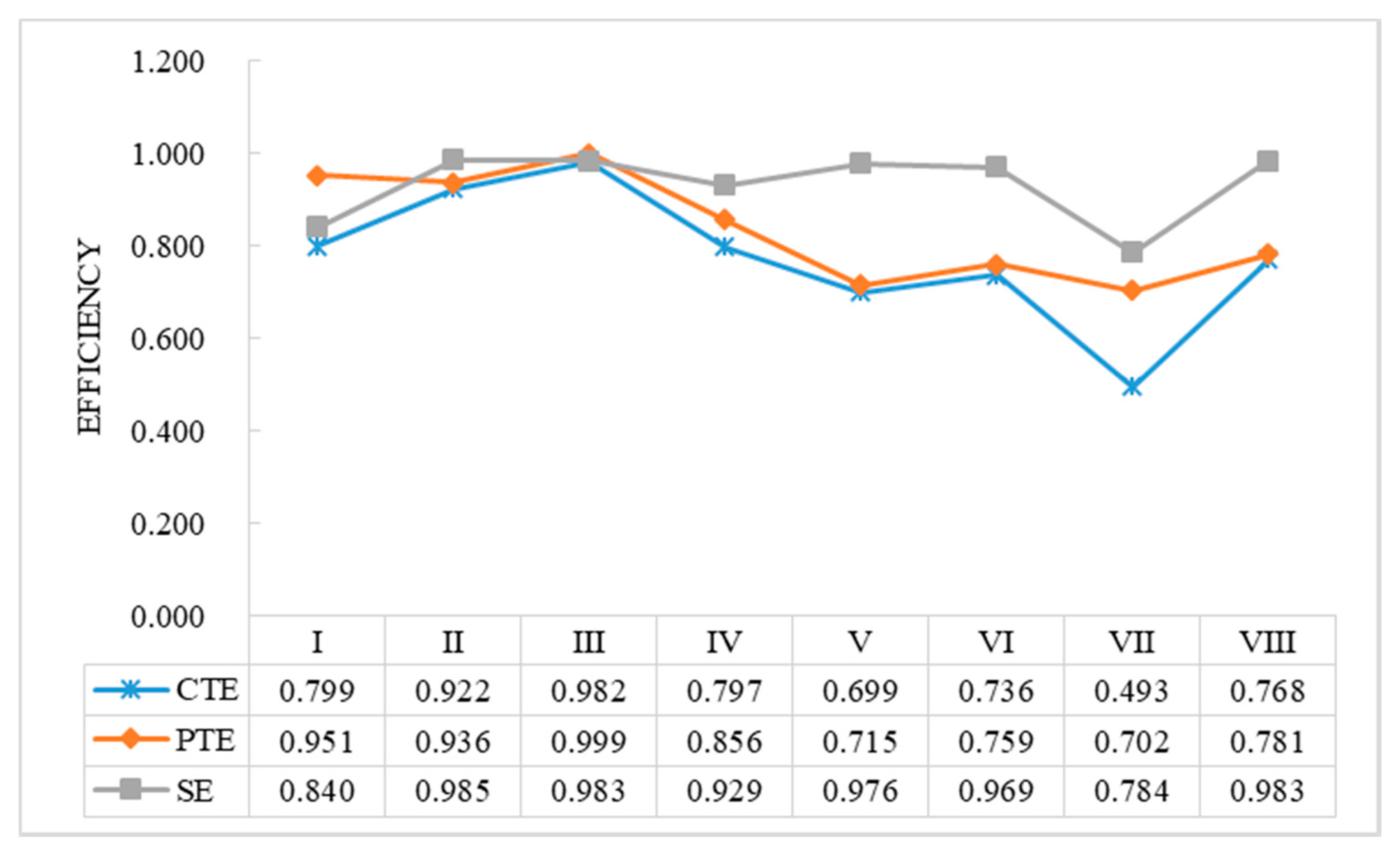
Region	The First Stage of DEA			The Third Stage of DEA
	CTE	PTE	SE	CTE	PTE	SE
I	0.799	0.951	0.840	0.912	0.964	0.945
II	0.922	0.936	0.985	0.823	0.953	0.868
III	0.982	0.999	0.983	0.995	0.999	0.996
IV	0.797	0.856	0.929	0.851	0.897	0.935
V	0.699	0.715	0.976	0.676	0.798	0.855
VI	0.736	0.759	0.969	0.729	0.815	0.900
VII	0.493	0.702	0.784	0.332	0.767	0.475
VIII	0.768	0.781	0.983	0.521	0.848	0.626
Mean	0.798	0.847	0.946	0.776	0.886	0.873

and

Table 5. The annual average of efficiency in China’s eight regions (3rd stage).

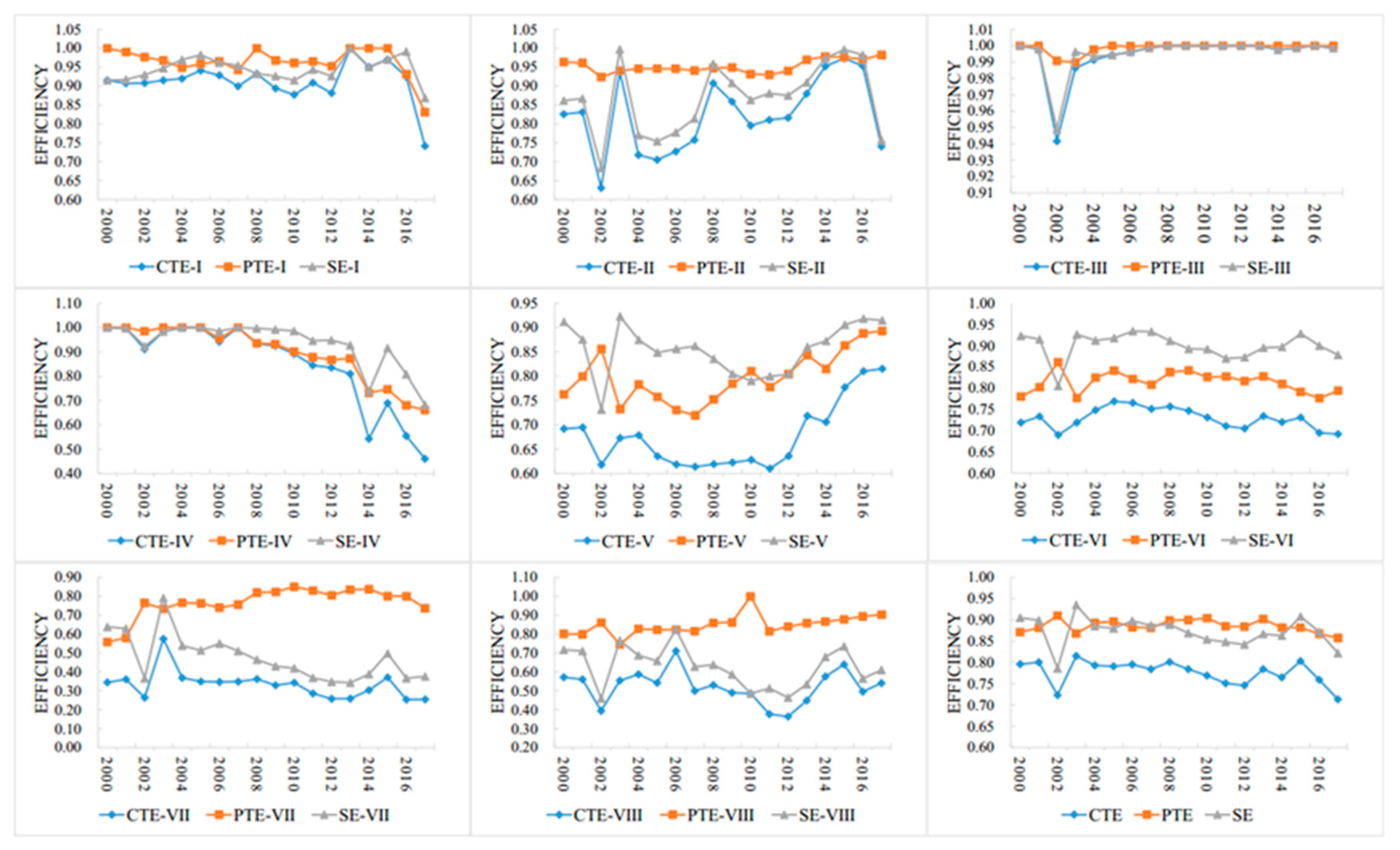
Year	I	II	III	IV	V	VI	VII	VIII
2000	0.915	0.826	1.000	1.000	0.692	0.719	0.345	0.572
2001	0.907	0.831	0.998	0.998	0.695	0.733	0.361	0.561
2002	0.908	0.631	0.942	0.911	0.618	0.690	0.265	0.395
2003	0.915	0.939	0.987	0.984	0.673	0.719	0.576	0.554
2004	0.920	0.718	0.991	1.000	0.678	0.748	0.369	0.587
2005	0.941	0.705	0.994	1.000	0.635	0.769	0.350	0.543
2006	0.928	0.727	0.996	0.942	0.618	0.765	0.348	0.711
2007	0.900	0.758	0.999	1.000	0.614	0.751	0.349	0.500
2008	0.932	0.908	1.000	0.934	0.619	0.757	0.363	0.530
2009	0.894	0.859	1.000	0.926	0.622	0.747	0.330	0.491
2010	0.877	0.796	1.000	0.892	0.628	0.731	0.343	0.486
2011	0.909	0.811	1.000	0.845	0.610	0.711	0.287	0.377
2012	0.882	0.816	1.000	0.836	0.636	0.705	0.259	0.364
2013	1.000	0.880	1.000	0.810	0.718	0.734	0.259	0.449
2014	0.950	0.953	0.998	0.543	0.705	0.720	0.304	0.576
2015	0.970	0.973	0.999	0.690	0.777	0.731	0.371	0.640
2016	0.925	0.953	1.000	0.554	0.810	0.695	0.255	0.496
2017	0.741	0.740	0.999	0.460	0.815	0.692	0.255	0.541

.

Overall analysis: After excluding environmental factors and random error factors, China’s annual average CEE of 0.798 was lower than that in the first stage (0.776), which was 22.4 percentage points different from the production frontier, mainly because the decline of SE value (7.7%) was higher than the increase of PTE value (4.6%). From the perspective of time, during 2000–2017, the CEE value was lower than that of the first stage in most years, and the opposite phenomenon only appeared in a few years. The average national CEE fluctuated around 0.776, but, due to the downward pressure on the national economy, it began to decline after 2015.

Comparing the efficiency distribution, it was found that after adjustment, only the CEE values of Regions I, II, and IV improved, and the efficiency values of all other regions declined to a certain extent, which may be due to better luck and favorable environment before being adjusted; it cannot show the absolutely high technical efficiency and management level. The main source of the decline in the value of CEE was the large-scale reduction in scale efficiency. The declines in Regions II, V, VI, VII, and VIII were 11.8%, 12.4%, 7.1%, 39.4%, and 36.3%, respectively. The size of the scale severely restricted the improvement of CEE. It can be seen that the scale of Gansu, Qinghai, Hainan, and Guizhou was too low. Moreover, the influencing factor of the adjusted efficiency value was the change from pure technical efficiency to scale efficiency.

From the regional perspective, on the whole, the CEE values of the eight regions steadily fluctuated around their annual averages from 2000 to 2017. The trend of efficiency change in Region II and Region VII was the same, and the trend of efficiency change in the period of 2001–2004 showed as a "down-rise-down" inverted N-type changing trend, which exactly matched the 10th Five-Year Plan period. In the process of accelerating industrial reorganization and transformation, optimizing industrial and energy structure, integrating advantageous industries, improving energy utilization efficiency, and strengthening environmental protection, provinces such as Gansu and Qinghai continued to probe development so that they caused fluctuation in regional CEE from 2001 to 2004. Since 2015, the regional coordinated development strategy of China has been gradually implemented, and some developed provinces have paid more attention to low-carbon economy and environmental protection. For example, Regions III and V were reflected clearly, and their efficiency values have been rising.

In Figure 3, the efficiency distributions of the eight regions in 2000–2017 are shown. The adjusted CEE rankings of the eight regions were still in different ranges, and the average efficiency rankings were as follows: Regions III, II, I, IV, VIII, VI, V, and VII. There is no ranking change, the ranking basically shows the downward trend of eastern, central and western China. The highest CEE value was in Region III (0.995), where there was an increase of 1.3% from the first stage, mainly due to the increase in scale efficiency of Anhui and Fujian provinces, indicating that it was not the absolute lowest in the first stage. In 2002, the efficiency value of Region III dropped sharply due to the low scale efficiency (0.802 and 0.892) of Anhui and Fujian Provinces, which were 15.1% and 10.8% lower than the first stage. The reason was the attempts of the two provinces to cope with how to persist and expand development scale. Moreover, the trends of CEE in all regions were consistent with scale efficiency. For example, due to the scale efficiency, Regions V and VI had abnormal points in 2002. Although the pure technical efficiency improved, the scale efficiency decreased more significantly (16.5% and 12%, respectively), so the CEE was a local minimum. In Region IV, Inner Mongolia, Xinjiang and Shaanxi are included. Region IV ranked high because Xinjiang was in the forefront of efficiency for most of the year in the observation period. Although the economic development level of Xinjiang was not high, it could comprehensively utilize existing resources and technologies to achieve a high level of CEE. This shows that the efficiency of economically developed regions is not necessarily high, however, the efficiency of economically underdeveloped regions also reaches the frontier, which may be related to the rational allocation of economic development, resource endowment, current management level, and so on, rather than just depending on the level of economic development.

5.2. Dynamic Analysis of the Three-Stage DEA-Malmquist Index Model

The DEA-Malmquist index of energy carbon emission in eight regions of China from 2000 to 2017 was analyzed. Then the results of total factor productivity (TFP) change, technological progress change (Tech), and technological efficiency change (Effch) of energy carbon emissions in each region and province were obtained. Comparing the Malmquist index of the first stage with the third stage, there were obvious differences in the study period, as shown in

Table 6. The comparison of total factor productivity (TFP) from 1st to 3rd stages in China’s eight regions.

Region	Malmquist Index in First Stage					Malmquist Index in Third Stage
	Effch	Tech	Pech	Sech	TFP	Effch	Tech	Pech	Sech	TFP
I	0.989	0.962	0.979	1.010	0.953	0.985	0.919	0.989	0.996	0.908
II	0.988	0.927	1.003	0.985	0.918	0.987	0.928	1.001	0.985	0.918
III	1.001	1.006	1.000	1.001	1.007	1.000	0.975	1.000	1.000	0.975
IV	0.956	0.895	0.961	0.995	0.856	0.953	0.868	0.975	0.977	0.828
V	1.016	1.006	1.014	1.002	1.023	1.010	0.974	1.009	1.000	0.982
VI	0.999	1.020	0.997	1.002	1.018	0.997	0.995	1.001	0.997	0.992
VII	0.987	0.962	1.005	0.983	0.950	0.976	0.912	1.016	0.960	0.890
VIII	1.010	0.954	1.010	1.000	0.964	0.999	0.921	1.009	0.990	0.920
Mean	0.994	0.978	0.996	0.999	0.973	0.991	0.949	0.999	0.991	0.940

,

Table 7. The annual TFP values in the 1st stage in China’s eight regions.

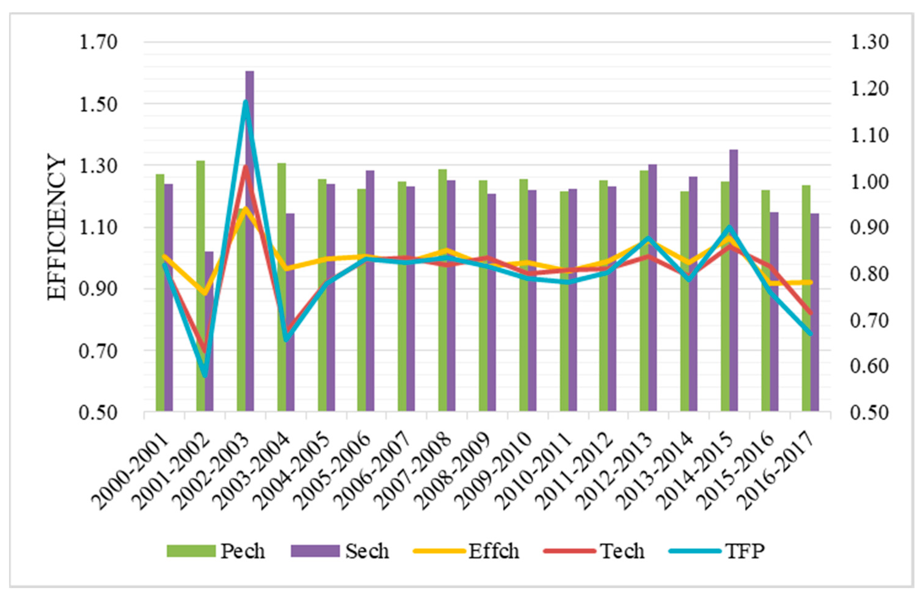
Period	I	II	III	IV	V	VI	VII	VIII
2000–2001	1.100	0.986	1.060	0.950	0.997	1.058	1.010	0.977
2001–2002	0.972	0.915	0.999	0.896	0.994	0.975	0.929	0.899
2002–2003	0.997	0.855	1.002	0.863	0.932	0.970	0.926	0.823
2003–2004	0.996	0.941	0.985	0.836	0.957	0.980	0.908	0.949
2004–2005	0.997	0.958	1.000	0.906	0.995	1.040	1.021	1.037
2005–2006	0.999	0.958	1.042	0.833	1.004	1.051	0.967	0.914
2006–2007	1.027	0.965	1.017	1.015	1.012	1.027	0.987	0.917
2007–2008	1.041	1.002	1.040	0.921	1.031	1.054	0.992	1.016
2008–2009	1.022	0.971	1.048	0.944	1.087	1.058	1.064	1.012
2009–2010	0.947	0.895	0.989	0.857	1.003	0.951	0.948	1.613
2010–2011	0.968	0.896	1.021	0.775	1.055	1.038	0.859	0.592
2011–2012	0.924	0.957	1.052	0.828	1.120	1.077	0.889	1.017
2012–2013	1.028	0.990	1.014	0.862	1.135	1.042	0.933	1.068
2013–2014	0.901	1.010	1.003	0.778	0.993	1.019	1.038	0.991
2014–2015	0.880	0.976	1.012	1.043	1.075	0.994	0.976	0.979
2015–2016	0.966	0.945	0.978	0.808	1.036	0.983	0.892	1.069
2016–2017	0.747	0.671	0.888	0.642	1.003	1.003	0.865	0.982
2000–2017	0.971	0.935	1.009	0.868	1.025	1.019	0.953	0.991

and Figure 4.

From a nationwide perspective, it was observed that the adjusted average change of the TFP, technological progress, and technological efficiency were lower than the corresponding values in the first stage from 2000 to 2017. After adjustment, the overall objectivity of CEE and the correctness of management decisions was higher, the average Malmquist index of China’s energy carbon emissions was 0.940, with an average growth rate of negative 6%. The main reason lay in the low efficiency of technological progress (0.949), and the low scale efficiency of technological efficiency (0.991) was another reason for inhibiting the growth of TFP. It indicates that the importance of the technological progress nationwide is not enough, and the management level and the allocation of factors are also not reasonable. So, it is urgent to increase the effective investment in improving the technological progress factors, and to expand and promote the economic development of the production scale at the same time.

In Figure 4 and Table 7, it can be found that the adjusted Malmquist indexes basically declined in different amplitudes. The trend of technological progress was consistent with that of TFP, and technological progress fluctuated in amplitude over a period of five years. Taking 2000 as the base period, the value of TFP was set as 1, and there were two partial volatility periods and a stable period in 2000–2017. From 2001 to 2005, the amplitude of TFP was large, showing a “W” type. From 2012 to 2017, TFP also fluctuated up and down, showing an “M” type. From 2006 to 2012, the change of TFP was relatively stable, slightly floating around 1.

There were three main reasons for the above changes. Firstly, in the period of the 10th Five-Year Plan (2000–2005), China implemented the basic concept of “development is the fundamental principle,” where all provinces were trying to increase productivity and expand production. During the period of 2002–2003, a series of environmental protection regulations was proposed, such as the Law of the People’s Republic of China on Cleaner Production Promotion Law, which made all production enterprises focus on the input of clean energy and raw materials, and the development of advanced processes and equipment. Not only was TEch greatly improved (1.297), but resource utilization efficiency and productivity improved, resulting in a sharp increase in TFPch from 2002 to 2003. Secondly, due to the downward pressure of the global economy in 2012 and the “Supply-side Structural Reform” implemented in 2015, TFP fluctuated up and down during this period. After 2015, TFP began declining year by year. Thirdly, technological progress floated slightly in 2007–2009, mainly because of the global economic crisis in 2007. Therefore, in the face of a shrinking market for domestic enterprises, only by increasing investment in research and development, continuously improving technology, and innovating new products, technology progress improved significantly in 2009.

From regional perspective, it can be seen from Table 6 that, before adjustment, the TFPs of Regions III, V, and VI were all greater than 1, but, after adjustment, the TFPs of the eight regions declined in different degrees, and the values were all lower than 1, which indicated that productivity had declined and the root cause was the corresponding technological regression caused by the mismatch between the existing development scale and external environmental impact. The adjusted ranking of TFP changed from Regions V, VI, III, VIII, I, II, VII, IV to Regions VI, V, III, VIII, II, I, VII, IV, which roughly matched the trend of eastern, central, western China. The lowest TFP of Region IV was 0.828, which was mainly due to the low level of technological progress in Inner Mongolia, Shaanxi, and Xinjiang. So it is important to pay attention to how to improve the region’s technological level and comprehensive application level with sufficient scale. The highest TFP of Region VI was 0.992, which was still 0.8% away from the frontier of production. Region VI includes Shanghai, Hebei, Henan, Heilongjiang, Guangxi, Tianjin, Jiangxi, Hubei, which are mainly distributed in the eastern and central regions, benefiting from their advanced economic level, rich energy resources, and advanced technology and equipment.

It can be seen in Table 7 that during the observation period, the changes in the total factor production of the eight regions in the first stage were relatively gentle and had the characteristic of consistent trend, all of which fluctuated around their own mean (0.971, 0.935, 1.009, 0.868, 1.025, 1.019, 0.953, 0.991). After comprehensive consideration of various external environments, the TFP of each region changed significantly. As shown in Figure 5, the trend of this change was consistent with that of the whole country. Between 2002 and 2003, the TFP of each region increased significantly. Among them, Region VII and II were higher. The reason is that the TFP of Qinghai and Yunnan was relatively high. Yunnan expanded its production scale, and Qinghai introduced advanced technology and equipment and greatly improved its technological progress.

5.3. Econometric Analysis of CEE

The above results show that there is a close relationship between CEE and TFP, but some scholars believe that the improvement or reduction of CEE depends on the improvement or backwardness of TFP [7]. In order to further analyze the technology progress, pure technology efficiency, and scale efficiency impact on the total factor CEE, a regression model was constructed with the CEE of each province as the dependent variable and the change value of technology progress, pure technology efficiency, and scale efficiency as the independent variables. Each index of the DEA-Malmquist model is the relative ratio to the previous year, so the CEE is also used as the dependent variable. The specific regression model can be expressed as follows:

$$Cec{h}_{it}=C+{\alpha }_{1}Tec{h}_{it}+{\alpha }_{2}Pec{h}_{it}+{\alpha }_{3}Sec{h}_{it}+{\epsilon }_{it},$$

(7)

where i represent the province, t represent a particular year, $Cech,Tech,Pech$ and $Sech$ represent the growth rate of CEE, technological progress, pure technological efficiency, and scale efficiency, respectively. Besides, $C$ is the intercept, ${\alpha }_1$, ${\alpha }_2$ and ${\alpha }_3$ are the coefficients, ${\epsilon }_{it}$ is the random error. Therefore, we can analyze the domestic panel data from 2000 to 2017 by econometric methods and the results are shown in

Table 8. The regression result of CEE in China.

Variable	Correlation	Standard Error	z-Value	Model Specification
C	0.238 ***	0.052	4.607	Fixed effects model
Tech	0.033 **	0.021	1.608
Pech	0.593 ***	0.043	13.860	Adjusted R2 = 0.306
Sech	0.134 ***	0.020	6.700	D-W value = 2.220

Notes: ***, **, * denote that the estimated value of the coefficient is significant at 1%, 5%, and 10%, respectively.

.

As can be seen from the table above, each variable passed the significance test. During the observation period, the increase of technological progress and technological efficiency could improve CEE. When technological progress and technological efficiency increased by 1%, respectively, CEE would increase by 0.033% and 0.079%. Relatively, the contribution of technological progress to CEE was small, which may be related to the “rebound effect” of technological progress. On the one hand, technological progress can reduce energy consumption and improve CEE. However, on the other hand, it can also make energy expenditure decrease and energy prices fall. Thereby the increase of the demand for energy could promote carbon emissions and curb the improvement of CEE. In addition, a 1% increase in pure technology efficiency and scale efficiency would contribute to an increase in CEE of 0.593% and 0.134%. This also verified the conclusion of the third stage DEA, the increase in CEE mainly came from the improvement of pure technical efficiency. At the same time, it showed that CEE was closely related to management level, technology level, and adjustment of factor structure.

6. Research Conclusions and Suggestions

6.1. Research Conclusions

Based on the panel data of China’s eight regions from 2000 to 2017, this paper selected three-stage DEA and the DEA-Malmquist model to measure the CEE of each region and analyzed the regions’ differences and characteristics. The main findings of this research are as follows.

First, the results of SFA regression revealed that the level of economic development did not significantly improve the CEE, but the optimization of industrial structure, the rational allocation of energy structure, the promotion of government regulation and technological innovation, and the expansion of openness had a positive impact on China’s CEE.

Second, from the static analysis results, the CEE values of the eight regions steadily fluctuated around their annual averages. The variation trends of CEE within the regions were convergent, while the variations of CEE among regions were diverse, and they were all distributed stably in different ranges. After adjustment, only the CEE values of Regions I, II, and IV improved, and the efficiency values of all other regions declined to a certain extent, the scale efficiency was the main factor in suppressing the improvement of CEE. The ranking was Regions III, II, I, IV, VIII, VI, V, and VII, which basically showed the downward trend of eastern, central and western China.

Third, from the dynamic analysis results, the TFP of the eight regions declined in different degrees due to technological progress, which was the main restraining factor of TFP. In other words, technological regression was the main reason for the decline in TFP. After comprehensive consideration of various external environments, the TFP of each region changed significantly. Technological progress took five years as a fluctuation period, basically, which was similar to the change trend of TFP. The trends of the two fluctuation periods were “W” and “M” type. Additionally, the TFP ranking was Regions VI, V, III, VIII, II, I, VII and IV, which roughly matched the trend of change from east to west.

Fourth, due to the rebound effect, although the regression results showed that the increase in technological progress and technological efficiency can improve CEE, the contribution value of technological progress was relatively less. The increase in technical efficiency can promote the CEE greatly, mainly due to the great growth of pure technical efficiency.

6.2. Suggestions

Based on the above findings, this paper puts forward the following suggestions from the regional and national perspectives. There are different characteristics among the eight regions, therefore comprehensive consideration should be made to adjust the resource allocations of these regions, reinforce mutual reference and cooperation among regions, clarify the direction of technological improvement, and improve the production scale, so as to improve the value of CEE and narrow the CEE gaps among these areas. Moreover, the innovative clustering of carbon emission reduction could provide a new reference for China’s regional coordinated development strategy and sustainable development of the mixed energy environment and economy.

In Regions I and III, there are many provinces in central or coastal regions with a higher than average efficiency of 0.9. In order to narrow the gap with other regions to achieve coordinated development, these two regions should give full play to their leading model roles, to display their advantages to the optimum, and to provide reference for other regions. These regions should continue to strengthen the promotion of high-tech levels and the ability of independent innovation and improve the proportion of high and new technology industries in the industrial structure, so as to provide more development experience and technical equipment for other areas. At the same time, striving for sustainable growth of technological progress and increasing the promotion of scale economy level are also necessary.

In Region II and Region IV, most of the provinces are located in the central and western regions and have average efficiency values higher than 0.8. Although the economic development levels of most provinces are not high, their carbon emission efficiency values are at a high level, indicating that these provinces have achieved better allocation under the existing resources and technology levels. These regions should pay attention to the introduction of advanced technology, strengthen the promotion and application of existing high and new technologies, make full use of the region’s advantages in energy resources endowment, increase the proportion of renewable energy and clean energy, expand scale production, and achieve economies of scale to improve the CEE and environmental protection.

In Region V, most provinces are distributed in the southwestern and northeastern regions and have efficiency values above 0.6. The region should be committed to changing the energy-intensive and extensive mode of production, introducing advanced technologies, increasing investment in energy science and technology. Further, Jilin, Chongqing, and Sichuan should accelerate the transformation of traditional industries with advantages, adjust and optimize the industrial structure, and increase the development of strategic emerging industries with their own characteristics to improve the CEE and narrow the gaps with other regions.

There are many provinces in Region VI, which are mainly distributed in the eastern, central, and northeastern regions, and the efficiency values are higher than 0.7. The region should actively develop tertiary industry, promote the transformation and upgrade of industrial structure, vigorously develop modern service and other emerging industries. In addition, Hebei and Heilongjiang could promote the quality and efficiency of traditional equipment manufacturing industries, restrict backward production capacity and energy intensive industries, introduce more advanced technology, and enhance independent innovation ability. The region could also improve the existing comprehensive energy utilization so as to expand the scale of production.

The provinces in Regions VII and VIII are located in the northwestern and southern regions with the lowest efficiency values (no more than 0.6). These regions should give full play to their own advantages and acquire more advanced experience and technology from surrounding areas. These two regions, as the key support objects, should also increase the investment of capital, advanced equipment, and the introduction of high-quality talents, change the backward development mode and machinery and equipment, limit the transfer and expansion of "three high" industries, and strive to develop and utilize new energy as much as possible, so as to improve the CEE to a certain extent.

At the national level, due to the great differences in economic development levels, industrial structure, resource endowment and technological innovation among regions in China, the relative efficiency gap of energy carbon emission is large at present. Therefore, when the government decomposes the energy conservation and emission reduction objectives, it should fully consider the level of economic development, industrial structure, energy structure, technological innovation, openness, and the capacity of carbon emission reduction, so as to avoid the “one size fits all” phenomenon, then work out the emission reduction standards by regions, enterprises, and industries.

Firstly, various regions should break through administrative barriers, make full use of geographical proximity and spillover effects, strengthen the flow of energy resource elements, resources and technology sharing within and between regions. According to local conditions, they should optimize resource allocation in order to promote industrial transformation and upgrading. Secondly, the government should take into account the evolutionary trend of historical carbon emission efficiency and regional characteristics, rezone the regions on carbon emission reduction, and then propose targeted measures for each region. Thirdly, the government should pay attention to the rebound of energy consumption and control energy prices reasonably by using active fiscal policies in the process of intervening in the economic downturn. In order to avoid a sharp increase in energy demand, we should start with technological progress and industrial transformation, upgrading to promote economic development stably. Fourthly, enterprises and industry sectors should vigorously develop and utilize clean energy and renewable energy, reduce the use of traditional energy sources as much as possible, and develop and manufacture low-carbon and environmentally friendly products for residents. Finally, we should fully understand the impact of technological progress, resource allocation, and management level on CEE. The improvement of CEE is a comprehensive project, which requires the government, enterprises, and residents to take a variety of measures to promote the process of energy conservation and emission reduction.

References

- British Petroleum (BP). BP Statistical Review of World Energy 2019 Workbook; British Petroleum: London, UK, 2019. [Google Scholar]
- Meng, F.Y.; Su, B.; Thomson, E.; Zhou, D.Q.; Zhou, P. Measuring China’s regional energy and carbon emission efficiency with DEA models: A survey. Appl. Energy 2016, 183, 1–21. [Google Scholar] [CrossRef]
- Kaya, Y.; Yokobori, K. Environment, Energy, and Economy: Strategies for Sustainability; United Nations University Press: Brussels, Belgium, 1997. [Google Scholar]
- Pretis, F.; Roser, M. Carbon dioxide emission-intensity in climate projections: Comparing the observational record to socio-economic scenarios. Energy 2017, 135, 718–725. [Google Scholar] [CrossRef] [PubMed]
- Ferreira, A.; Pinheiro, M.D.; de Brito, J.; Mateus, R. Combined carbon and energy intensity benchmarks for sustainable retail stores. Energy 2018, 165, 877–889. [Google Scholar] [CrossRef] [Green Version]
- Song, J.Z.; Yuan, X.Y.; Wang, X.P. Analysis on influencing factors of carbon emission intensity of construction industry in China. Environ. Eng. 2018, 36, 178–182. [Google Scholar]
- Hu, J.L.; Wang, S.C. Total factor energy efficiency of regions in China. Energy Policy 2006, 34, 3206–3217. [Google Scholar] [CrossRef]
- Zhou, P.; Ang, B.W.; Han, J.Y. Total factor carbon emission performance: A malmquist index analysis. Energy Econ. 2010, 32, 194–201. [Google Scholar] [CrossRef]
- Song, M.L.; An, Q.; Zhang, W.; Wang, Z.; Wu, J. Environmental efficiency evaluation based on data envelopment analysis: A review. Renew. Sustain. Energy Rev. 2012, 16, 4465–4469. [Google Scholar] [CrossRef]
- Molinos-Senante, M.; Sala-Garrido, R.; Hern andez-Sancho, F. Development and application of the Hicks-Moorsteen productivity index for the total factor productivity assessment of wastewater treatment plants. J. Clean Prod. 2016, 112, 3116–3123. [Google Scholar] [CrossRef]
- Zaim, O.; Taskin, F. Environmental efficiency in carbon dioxide emissions in the OECD: A non-parametric approach. J. Environ. Manag. 2000, 58, 95–107. [Google Scholar] [CrossRef]
- Zofio, J.L.; Prieto, A.M. Environmental efficiency and regulatory standards: The case of CO2 emissions from OECD industries. Resour. Energy Econ. 2001, 23, 63–83. [Google Scholar] [CrossRef]
- Wang, Z.X.; Ye, D.J.; Zheng, H.H.; Lv, C.Y. The influence of market reform on the CO2 emission efficiency of China. J. Clean Prod. 2019, 225, 236–247. [Google Scholar] [CrossRef]
- Dong, F.; Long, R.Y.; Bian, Z.F.; Xu, X.H.; Yu, B.L.; Wang, Y. Applying a Ruggiero three-stage super-efficiency DEA model to gauge regional carbon emission efficiency: Evidence from China. Nat. Hazards 2017, 27, 1453–1468. [Google Scholar] [CrossRef]
- Tone, K. A slack-based measure of efficiency in data envelopment analysis. Eur. J. Oper. Res. 2001, 130, 498–509. [Google Scholar] [CrossRef] [Green Version]
- Choi, Y.; Zhang, N.; Zhou, P. Efficiency and abatement costs of energy-related CO2 emissions in China: A slacks-based efficiency measure. Appl. Energy 2012, 98, 198–208. [Google Scholar] [CrossRef]
- Gomez-Calvet, R.; Conesa, D.; Gomez-Calvet, A.R.; Tortosa-Ausina, E. Energy efficiency in the European Union: What can be learned from the joint application of directional distance functions and slacks-based measures? Appl. Energy 2014, 132, 137–154. [Google Scholar] [CrossRef]
- Iftikhar, Y.; He, W.; Wang, Z. Energy and CO2 emissions efficiency of major economies: A nonparametric analysis. J. Clean Prod. 2016, 139, 779–787. [Google Scholar] [CrossRef]
- Cecchini, L.; Venanzi, S.; Pierri, A.; Chiorri, M. Environmental efficiency analysis and estimation of CO2 abatement costs in dairy cattle farms in Umbria (Italy): A SBM-DEA model with undesirable output. J. Clean Prod. 2018, 197, 895–907. [Google Scholar] [CrossRef]
- Wang, Q.; Su, B.; Sun, J.; Zhou, P.; Zhou, D. Measurement and decomposition of energy-saving and emissions reduction performance in Chinese cities. Appl. Energy 2015, 151, 85–92. [Google Scholar] [CrossRef]
- Park, Y.S.; Lim, S.H.; Egilmez, G.; Szmerekovsky, J. Environmental efficiency assessment of U.S. transport sector: A slack-based data envelopment analysis approach. Transport Environ. 2018, 61, 152–164. [Google Scholar] [CrossRef] [Green Version]
- Zhou, Y.X.; Liu, W.L.; Lv, X.Y.; Chen, X.H.; Shen, M.H. Investigating interior driving factors and cross-industrial linkages of carbon emission efficiency in China’s construction industry: Based on Super-SBM DEA and GVAR model. J. Clean Prod. 2019, 241, 1–13. [Google Scholar] [CrossRef]
- Dong, F.; Li, X.H.; Long, R.Y.; Liu, X.Y. Regional carbon emission performance in China according to a stochastic frontier model. Renew. Sustain. Energy Rev. 2013, 28, 525–530. [Google Scholar] [CrossRef]
- Fried, H.O.; Lovell, C.A.K.; Schmidt, S.S.; Yaisawarng, S. Accounting for environmental effects and statistical noise in data envelopment analysis. J. Prod. Anal. 2002, 17, 121–136. [Google Scholar] [CrossRef]
- Jiang, S.R.; Tan, X.; Shi, L. Industrial air pollution emission efficiency in Beijing-Tianjin-Hebei and its surrounding areas-based on three stage DEA model. J. Arid Land Res. Environ. 2019, 33, 141–149. [Google Scholar]
- Wang, Y.; Cheng, L.W.; Wang, X.N. Financial Function Promotion and Dynamic Endogenous Club Convergence in Regional Financial Development. Oper. Res. Manag. Sci. 2019, 28, 142–156. [Google Scholar]
- Yang, C.Y.; Qi, Z.H.; Huang, W.H. Is agricultural social service conducive to the improvement of agricultural production efficiency? An empirical analysis based on three stage DEA model. J. Chin. Agric. Univ. 2018, 23, 232–244. [Google Scholar]
- Liu, Z.F.; Wang, C.H. Organic Agricultural Production Efficiency Based on a Three-stage DEA Model: A Case Study of Yang County, Shaanxi Province. Chin. J. Popul. Resour. Environ. 2015, 25, 105–112. [Google Scholar]
- Yin, J.Y.; Cao, Y.F.; Tang, B.J. Fairness of China’s provincial energy environment efficiency evaluation: Empirical analysis using a three-stage data envelopment analysis model. Nat. Hazards 2019, 95, 343–362. [Google Scholar] [CrossRef]
- Wang, Q.W.; Su, B.; Zhou, P.; Chiu, C.R. Measuring total-factor CO2 emission performance and technology gaps using a non-radial directional distance function: A modified approach. Energy Econ. 2016, 56, 475–482. [Google Scholar] [CrossRef]
- Mahmoudabadi, M.Z.; Emrouznejad, A. Comprehensive performance evaluation of banking branches: A three-stage slacks-based measure (SBM) data envelopment analysis. Int. Rev. Econ. Finance 2019, 64, 359–376. [Google Scholar] [CrossRef]
- Huang, H.F.; Wang, T. The Total-Factor Energy Efficiency of Regions in China: Based on Three-Stage SBM Model. Sustainability 2017, 9, 1664. [Google Scholar] [CrossRef] [Green Version]
- Jiang, C.B.; Li, S.F.; Li, L. Research on productive efficiencies measurement based on three-stage super DEA model: A case of Chinese road and bridge enterprises. Int. J. Comput. Sci. Math. 2017, 8, 475–493. [Google Scholar]
- Wang, Z.H.; Feng, C.; Zhang, B. An empirical analysis of China’s energy efficiency from both static and dynamic perspectives. Energy 2014, 74, 322–330. [Google Scholar] [CrossRef]
- Kortelainen, M. Dynamic environmental performance analysis: A Malmquist index approach. Ecol. Econ. 2007, 64, 701–715. [Google Scholar]
- Chen, S.B.; Feng, Y.Q.; Lin, C.R. Innovation efficiency evaluation of new and high technology industries based on DEA-Malmquist index. J. Interdiscip. Math. 2017, 20, 1497–1500. [Google Scholar] [CrossRef]
- Chen, Y.; Liu, B.S.; Shen, Y.H.; Wang, X.Q. Spatial analysis of change trend and influencing factors of total factor productivity in China’s regional construction industry. Appl. Econ. 2018, 50, 2824–2843. [Google Scholar] [CrossRef]
- Zheng, S.N.; Wang, S.Q.; Liang, Q. Total Factor Productivity and Decomposition of Fisheries Economy in Coastal Areas of the Mainland of China and Taiwan: Using the DEA-Malmquist Index. J. Coas. Res. 2019, 93, 371–380. [Google Scholar] [CrossRef]
- Sun, J.W.; Li, S.S.; Zhao, X.W. An empirical analysis on total factor productive energy efficiency of Yangtze River Delta region-based on DEA-Malmquist productivity index. Manual Eng. Environ. Eng. 2014, 84, 1003–1009. [Google Scholar]
- Sun, X. Analysis on Dynamic Changes of Efficiency of Regional Energy-saving & Emission Reduction in China. Comput. Eval. Econ. Soc. Stat. Sci. 2009, 992–996. [Google Scholar]
- Charnes, A.; Cooper, W.W.; Rhodes, E. Measuring the efficiency of decision making units. Eur. J. Oper. Res. 1978, 2, 429–444. [Google Scholar] [CrossRef]
- Banker, R.D.; Charnes, A.; Cooper, W.W. Some models for estimating technical and scale inefficiencies in data envelopment analysis. Manag. Sci. 1984, 30, 1078–1092. [Google Scholar] [CrossRef] [Green Version]
- Jondrow, J.; Lovell, C.A.K.; Materov, I.S. On the estimation of technical inefficiency in the stochastic frontier production function model. J. Econ. 1982, 19, 233–238. [Google Scholar] [CrossRef] [Green Version]
- Caves, D.W.; Christensen, L.R.; Diewert, W.E. The economic theory of index numbers and the measurement of input, output, and productivity. Econ. Soc. 1982, 50, 1393–1413. [Google Scholar] [CrossRef]
- Färe, R.; Grosskopf, S.; Norris, M. Productivity growth, technical progress and efficiency change in industrialized countries. Am. Econ. Rev. 1994, 84, 66–83. [Google Scholar]
- Chung, Y.H.; Fare, R.; Grosskopf, S. Productivity and undesirable outputs: A directional distance function approach. Microeconomics 1995, 51, 229–240. [Google Scholar] [CrossRef] [Green Version]
- Seiford, L.M.; Zhu, J. Modeling undesirable factors in efficiency evaluation. Eur. J. Oper. Res. 2002, 142, 16–20. [Google Scholar] [CrossRef]
- Shan, H.J. Reestimating the capital stock of China: 1951–2006. Quant. Tech. Econ. 2008, 10, 17–31. [Google Scholar]
- IPCC. 2006 IPCC Guidelines for National Greenhouse Gas Inventories: Volume II. Japan; The Institute for Global Environmental Strategies: Kanagawa, Japan, 2008. [Google Scholar]
- Wu, X.D.; Kumar, V. The Top Ten Algorithms in Data Mining; CRC Press: Boca Raton, FL, USA, 2009. [Google Scholar]
- Murtagh, F.; Contreras, P. Algorithms for hierarchical clustering: An overview. Wiley Interdisc. Rev. Data Mining Knowl. Discov. 2012, 2, 86–97. [Google Scholar] [CrossRef]