Abstract
It is necessary to develop a sustainable food production system to ensure future food security around the globe. Cropping intensity and sowing month are two essential parameters for analyzing the food–water–climate tradeoff as food sustainability indicators. This study presents a global-scale analysis of cropping intensity and sowing month from 2000 to 2015, divided into three groups of years. The study methodology integrates the satellite-derived normalized vegetation index (NDVI) of 16-day composite Moderate Resolution Imaging Spectroradiometer (MODIS) and daily land-surface-water coverage (LSWC) data obtained from The Advanced Microwave Scanning Radiometer (AMSR-E/2) in 1-km aggregate pixel resolution. A fast Fourier transform was applied to normalize the MODIS NDVI time-series data. By using advanced methods with intensive optic and microwave time-series data, this study set out to anticipate potential dynamic changes in global cropland activity over 15 years representing the Millennium Development Goal period. These products are the first global datasets that provide information on crop activities in 15-year data derived from optic and microwave satellite data. The results show that in 2000–2005, the total global double-crop intensity was 7.1 million km2, which increased to 8.3 million km2 in 2006–2010, and then to approximately 8.6 million km2 in 2011–2015. In the same periods, global triple-crop agriculture showed a rapid positive growth from 0.73 to 1.12 and then 1.28 million km2, respectively. The results show that Asia dominated double- and triple-crop growth, while showcasing the expansion of single-cropping area in Africa. The finer spatial resolution, combined with a long-term global analysis, means that this methodology has the potential to be applied in several sustainability studies, from global- to local-level perspectives.
1. Introduction
Researchers worldwide have been focusing on how to find a better approach to increasing food production in a more sustainable manner, as the food balance is predicted to exhibit a negative trend over the next decade due to increasing global demand [1,2]. Sustainable crop production refers to agricultural production in such a way that it does not cause any harm to the environment, biodiversity, or quality of agricultural crops [3,4]. According to a report published by the United Nation Department of Economic and Social Affairs (UN DESA) [5], the global population will reach 8.5 billion in 2030. Consequently, studies have estimated a need to increase food production by 60% using 1.2 million km2 of converted land [6,7,8]. A common solution to increasing food-crop production involves expanding the cropland area. However, current cropland areas are shrinking owing to urbanization, industrialization, and prevailing drought crises [9,10]. Therefore, several countries have tried to intensify their use of cultivated lands. This strategy provides a promising means of improving global crop production without the need to increase the amount of agricultural land [11,12]. However, to ensure sustainability, food security must consider the tradeoff between food production, water demand, and emissions [13,14]. High cropping-intensity agriculture incurs high risks due to the adverse effects of increased water demand and greenhouse gas (GHG) emissions [15,16]. When evaluating the progress toward achieving sustainable development goals (SDGs), it is essential to develop sustainable and accurate data metrics, such as the long-term global cropping intensity and the crop calendar [17,18]. The crop calendar is defined as the times at which farmers are sowing and harvesting crops, and cropping intensity refers to the number of cropping cycles per year [11]. These two important parameters allow researchers to consider not only the volume of food production, water demand, and emissions, but also the time required to accommodate dramatic changes in production demand. This information has potential applications for policy makers tasked with monitoring and implementing interventions. Several previous studies have applied these crop activity parameters to fight hunger, water crises, and climate change. Ray et al. [19] applied the parameters in estimating and projecting future yield. Doll and Siebert [20] and Wada et al. [21] used cropping intensity and calendar to calculate the global crop water requirement in pixels. Studies related to global ground water modeling, as presented by Oki and Kanae [22], also applied cropping activity to surface information as one of the significant inputs. The latest study that used these parameters was a scenario modeling of global agriculture redistribution by Davis et al. [23]. These studies show that improving cropping-intensity and calendar products will benefit future research and support strategic policies. There are three existing approaches to estimating these crop-activity parameters: census-based, model simulation, and remote sensing. The limitations of these approaches, considered below, point to the need for more research in order for SDGs to be met.
The global dataset of Monthly Irrigated and Rainfed Crop Areas Around the Year 2000 (MIRCA) [24] is a global crop database of monthly growing areas for 26 irrigated and rainfed crops. The database combines a census-based approach and existing statistical database, such as the Food and Agriculture Organization (FAO) irrigated area statistics. The dataset covers the period 1998–2002 and has a spatial resolution of 5 and 30 arc-min. As the information is directly obtained from the census data, the product has an advantage in terms of data quality compared with other products. The MIRCA dataset includes: (1) the number of crops, (2) the maximum area occupied by each individual crop, (3) the most, second-most, third-most, fourth-most, and fifth-most important global major crops (based on the criterion of the amount of area planted with the particular crop globally), (4) the ratios of rainfed and irrigated crops in the crop mix, and (5) the crop calendars. However, a limitation of this product lies in the distribution of the survey, as poor access to certain areas makes it difficult to collect information. Further, statistical data with small spatial units can produce low-sensitivity data. As a high-quality census distribution is costly, some studies have used interpolation strategies to produce a profile of an unknown area [25]. Because of this limitation, a census-based approach produces large uncertainties in the crop calendar and cropping intensity information, especially for global-scale analysis [26]. Model-based simulation and remote-sensing techniques have the potential to reduce these uncertainties, as these approaches are able to monitor large-scale areas.
Model simulation-based approaches, such as those used by Waha et al. [27] and Zabel et al. [28] (in this study, WAHA refers to Waha et al. [27] and ZABEL refers to Zabel et al. [28] study product), can simulate global cropping intensity and crop calendars by using meteorological forecasting data. This method reflects specific climate requirements and topographic characteristics. The model considers that climatic conditions, such as rainfall and temperature, affect the planting date, which is important because several studies have shown a strong relationship among the climate, soil, topography, and agricultural suitability [29,30]. The best feature of the model-based approach is that projection modeling is possible with a high temporal resolution. For example, ZABEL released a crop-suitability product for two periods, namely, 1981–2010 and 2071–2100. However, the accuracy of this product depends on the quality of its base map and climate model, which vary considerably depending on the model type and parameter input [31,32].
The advantage of remote sensing is its capacity for high-reproducibility spatial data over a large coverage area with various applications, produced in a timely manner [33]. However, the quality of datasets gathered by remote sensing depends on the spatial, spectral, and temporal characteristics of each satellite sensor. Based on the characteristics of radiation source, spectral radiance, and electromagnetic spectrum, the remote-sensing system is divided into optic, thermal, and microwave sensors. In general, optic and thermal sensors measure reflected and emitted energy in visible and thermal wavelengths. On the other hand, a microwave sensor measures the time distance between the sensor and an object. To overcome this limitation, several studies have tried to integrate multisatellite datasets according to the strength of different sensors of the optic and microwave types [34,35]. The Satellite-derived Crop Calendar for Agricultural Simulations (SACRA) product [36] can obtain the recent cropping intensity and crop calendar by using the time series of vegetation index derived from Satellite Pour l’Observation de la Terre (SPOT) satellite imagery. The strength of the SACRA product is its integration of remote sensing, census-based MIRCA, and temperature data obtained from the H08 model [37]. However, the products only use single optical satellite data, produced with a coarse pixel resolution of 5 arc-min or 10 km at the Equator, and the SACRA product can only present data from one representative year as single data that represent the averaged Normalized Different Vegetation Index (NDVI) over 3 years (2004–2006). Therefore, this dataset cannot be used for analyzing data in terms of multiyear crop change.
The limitations of these current products demonstrate the need to develop a method for analyzing long-term crop activity through multisatellite integration for enhancing product quality. In particular, to monitor crop phenology, the current approach of using a dominant optic base must be enhanced to use other satellite data, such as those produced using radar. Thus, the main objective of this study was to develop long-term, moderate-resolution data representing the global cropping intensity and sowing month in a 30 arc-second spatial resolution (approximately 1 km at the Equator). We set out to fill the information gap by estimating these two crop-activity parameters for a 15-year analysis covering the period 2001–2015, divided into three blocks of five consecutive years.
2. Materials and Methods
We explored the potential integration of the satellite-derived NDVI from Moderate Resolution Imaging Spectroradiometer (MODIS) and land-surface-water coverage (LSWC) from The Advanced Microwave Scanning Radiometer (AMSR-E/2) to analyze the crop-phenology information. By using advanced methods of intensive optic and microwave global data processing with time series analysis using a multi-core processor on High Performance Computing (HPC), this study set out to anticipate potential dynamic changes in global cropland activity over 15 years representing the Millennium Development Goal (MDG) period. The novelty of this study is that it is the first to develop global datasets that provide information regarding cropping intensity and sowing month using 15 years of data derived from the integration of optical and microwave satellite imagery.
For estimating the cropping intensity, we used only MODIS NDVI, which was integrated with the International Institute for Applied Systems Analysis (IIASA) cropland fraction as the base map. In this study, we named it the “MODIS cropping intensity” (MODIS CI) product; it indicates the estimated number of cropping cycles per year. For crop calendar analysis, we only focused on detecting the sowing month without detecting the harvesting date. For this analysis, the product was named “MODIS-AMSR sowing month”, as it was a combination of the MODIS NDVI and AMSR-E/2 LSWC, and used for data processing. Since there are no available data using a higher spatial resolution with extensive ground base data, we applied some comparative analysis of our cropping-intensity and sowing-month products with spatial and statistic data. For cross-comparison with spatial data, we compared our MODIS-AMSR sowing-month product with MIRCA, SACRA, and ZABEL products. This cross-validation analysis aimed to check the consistency and different trends among data products. For statistics-based comparison, we calculated the total area of double- and triple-crop intensity in 162 countries from four cropping-intensity products and compared it with the irrigated FAO-stat of the irrigated areas [38]. To support this comparative study, we used Historical, gridded land use (HYDE 3.2) irrigated crop area [39] for visual comparison to look at how correlations between non-single-cropping intensities are predominantly located in irrigated areas. This section describes the materials and methods applied to produce MODIS CI and MODIS-AMSR sowing month. Figure 1 shows the data-processing schemes of MODIS and AMSR-E/2. The following subsections explain the data used in the present study: MODIS NDVI and AMSR-E/2 LSWC (Section 2.1). Subsequently, we describe the strategies for estimating the cropping intensity (Section 2.2) and sowing month (Section 2.3). Finally, Section 2.4 explains the approach for harmonizing previous global crop products.
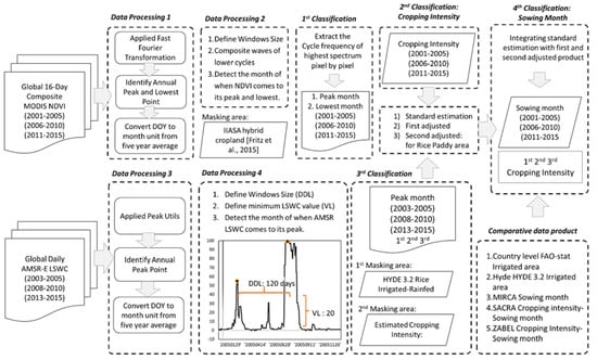
Figure 1.
Data-processing scheme of the MODIS-AMSR cropping intensity and sowing month.
2.1. Data Used in This Study
2.1.1. MODIS NDVI Data Processing
In the present study, we investigated the time series of the satellite-sensed MODIS NDVI (MOD13A2) 16-day composite with a 1-km spatial resolution. Satellite-driven vegetation indices (VIs), such as NDVI, have been widely used to monitor crop profiles such as phenology, amount of leaves, and biomass [40]. Specifically, several studies have conducted spectral analyses of time-series NDVI to estimate the crop extensification [41], number of cropping intensities [36,42,43], and crop calendar [44,45]. We prepared NDVI data in the MOD13A2 product from the beginning of 2001 to the end of 2015, and divided the archived data for these 15 years into three groups of five consecutive years: 2001–2005, 2006–2010, and 2011–2015 (Figure 2a). This study included 115 samples from each of the three year groups, with a total of 315 global MODIS NDVI datasets. MODIS-NDVI can be calculated as follows:
where VIS represents the reflectance value of the red visible channel, 0.620–0.670 µm (Channel 1), and NIR represents the near-infrared channel of 0.545–0.564 µm (Channel 4). This equation is based on the abilities of VIS and NIR to absorb chlorophyll and scatter the mesophyll leaf structure, respectively [46].
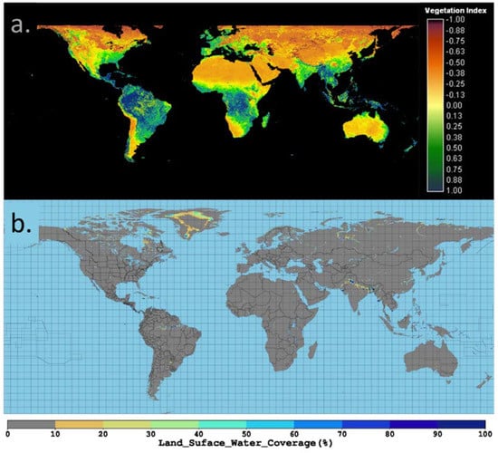
Figure 2.
Global products of (a) 16-day composites of MODIS normalized vegetation index (NDVI) and (b) daily AMSR-E/2 land-surface-water coverage (LSWC).
2.1.2. AMSR-E and AMSR-2 LSWC Data Processing
To monitor crop phenology, the current approach of using MODIS NDVI must be enhanced such that other satellite data can be used. A next-generation geostationary satellite with daily data acquisition and a microwave-observation sensor has the potential to be integrated with a MODIS optic base sensor. Further, advanced microwave-scanning radiometers (AMSR), such as AMSR-E and AMSR-2, could be powerful tools for monitoring water surface patterns and avoiding cloud contamination [47]. A key feature of these AMSR instruments is their ability to see through clouds, thereby providing an uninterrupted view of the land measurements, especially in the rainy season [48]. Moreover, such sensors have the advantages of both sensor and daily temporal resolutions. This means that they have the potential to monitor flooding sessions in rice paddy fields. To meet the 1-km product target, that is, the same as MODIS, we reanalyzed the nearest 30 arc-second grid from AMSR-E/2 5 arc-min grids.
AMSR-E/2 LSWC is a function of the combination of the normalized difference frequent index (NDFI) and normalized difference polarization index (NDPI) of AMSR-E/2 [49]. NDFI and NDPI provide a sensitivity indicator to detect the presence of surface water, and they can distinguish water and land surfaces [50]. To extract NDPI and NDFI, we used AMSR-E/2 level-3 data, which consist of brightness temperatures observed from an ascending orbit. When the atmospheric transmission is near to that of 1 AMSR-E/2, NDFI and NDPI can be calculated using Equations (2) and (3), respectively. BT36.5H is the horizontal (H) polarization brightness temperature at 36.5 GHz, and BT23.8V, BT18.7V, and BT36.5V are the vertical (V) polarization brightness temperatures at 23.8, 18.7, and 36.5 GHz, respectively. The LSWCs of AMSR-E and AMSR-2 were mapped, and exponential functions were obtained with NDFI and NDPI, and expressed using Equation (4).
Several potential applications of AMSR-E/2 LSWC that are effective for the monitoring of agricultural issues, especially the flooding sessions in rice paddy phenology, have been proposed [51]. AMSR-E/2 LSWC can also be applied to large-scale flooding detection [52]. Figure 2b shows an LSWC product derived from AMSR-E and AMSR-2, with the value ranging from 0% to 100% indicating the water-cover fraction in each pixel dataset. The transition from AMSR-E to AMSR-2 resulted in several missing data, and thus data from all 15 years could not be used. To ensure that each group of years had the same amount of data, we considered three groups obtained from three consecutive years, i.e., 2003–2005 and 2008–2010 for AMSR-E, and 2013–2015 for AMSR-2.
2.2. Cropping Intensity Estimation
We used a fast Fourier transform (FFT) to normalize the NDVI time-series process from the interference of cloud contamination and spectral mixture. The Fourier transform has proven to be a powerful tool for classifying cloud-affected data in remote-sensing imagery [53]. FFT is a mathematical operation that aims to decompose a time-domain signal to a frequency-domain signal. FFT implements the discrete Fourier transform (DFT) with a calculation technique that utilizes the periodic properties of a Fourier transform [54]. The basic principle of the algorithm is the decomposition of the FFT calculation from a long sequence, N, into smaller FFTs in a row [55]. This normalizes the NDVI of the crop phenology to detect the cropping pattern, and is expected to reduce uncertainty in identifying the peaks and troughs in NDVI phenology [56]. Here, a peak is defined as the highest NDVI value between the lowest points of the NDVI phenology, while a trough is defined as the lowest NDVI value between the highest NDVI values. The FFT equation is expressed as follows:
where k denotes the data value, and N is the number of 16-day MODIS NDVI samples. The FFT result indicates the power spectrum revealing the crop intensity and timing. The frequency of the highest spectrum is defined as the number of cropping cycles in a pixel. For cropping-intensity estimation, we assume the number of NDVI peaks in a year to be the required information. Our strategy involves the analysis of NDVI phenology in each of the 5-year groups to produce a more accurate real cropping intensity. After the cropping cycles for 5 years had been counted, we aligned all the cycles to obtain the average cropping per year. We assume that the NDVI time series represents the phenology of one dominant crop in each grid. The peak (Equation (6)) and trough (Equation (7)) points can be detected over the range between the highest and lowest values, and are expressed as:
The selected peak (tpk) and trough (ttrg) points are calculated by comparing each value within 48 days (3 NDVI data) before and after the peak and trough point candidates. These processes were conducted throughout the global cropland base map, i.e., the 1-km International Institute for Applied Systems Analysis-The International Food Policy Research Institute (IIASA-IFPRI) cropland fraction product [57], pixel by pixel, with 51,535,433 cropland pixels in total. This hybrid cropland, with the baseline year being 2005, was developed by integrating a number of individual, global, and regional cropland maps. The IIASA data were selected as the base map because they had been recently collated and provide a highly accurate area of the global cropland fields at the same 1-km pixel resolution. We implemented the same base map for all the three data groups by assuming that the cropland-expansion-change phenomena over 15 years occurred only within the existing pixel fraction.
2.3. Sowing-Month Estimation
To detect the peak of the time-series data, data processing by AMSR-E/2 LSWC and MODIS NDVI differs because FFT analysis is not applied in the AMSR-based data processing. This could be because the time-series data of AMSR-E/2 LSWC can potentially detect flat patterns, implying that the FFT process cannot work well for normalizing the pattern [58]. Moreover, the radar sensor based on the AMSR series data causes the time-series product of the water surface to be free from climate interfaces, such as rainfall and cloud cover. We analyzed the peak average in each year group by using the Peak Utils 1.3 package tool [59], a python library developed by Massachusetts Institute of Technology (MIT) that can be used to detect peaks and troughs in time-series datasets of certain wavelengths. This package provides utilities related to peak detection in 1D data, and also includes functions for finding the peak indexes in the data and performing Gaussian fitting to further increase the resolution of peak detection. For detecting peaks during flooding sessions in a rice paddy field, we define two parameters: (1) window size (DDL) and (2) minimum LSWC (VL) value. After several tests, we estimated the recommended values of the minimum length between peaks (DDL) and LSWC (VL) as 120 days and 20%, respectively. Visualizations of the DDL and VL parameters in the AMSR LSWC data processing are shown in Figure 1 (data processing 4). This decision was based on the minimum requirement value that can be used to clearly identify peaks during the rice paddy flooding session. By considering this threshold, the peak in AMSR-E/2 LSWC was analyzed to detect true flooding and thus estimate the single- to triple-crop intensity of rice paddies.
After developing the peak month product from the AMSR long-term data processing, we applied pixel upscaling without interpolation [27,36] to reduce the arc-min product size from 10 km to 1 km without changing the original number of data. The processes for upscaling the data were applied after we developed the peak month product to minimize the error incurred by the detection of the spatial heterogeneity inside the new 5 arc-min product. Using the same technique, we applied harmonization of the previous cropping-intensity and sowing-month products to attain the same level as the MODIS-AMSR cropping-intensity and sowing-month products.
Previous approaches used to detect the sowing month are as follows: (1) detection two months before the appearance of the VI peak (CROPWAT) and 2:1-month approach (i.e., two months from planting to peak and one month from peak to harvest) [60]; (2) combining the trough point of VI with the climate data [29]. However, the estimation of the sowing month two months before the peak is a very simple assumption, and the identification of the trough point as a reference is very risky, as it is estimated through cloud contamination [61]. In the present study, we propose three approaches to estimating the global sowing month for both rice and non-rice crop types. We also used information on double- and triple-cropping areas for estimating the sowing month in the first, second, and third cultivation periods. (1) In the standard approach, the general crop cultivation time was derived from the CROPWAT model, where the planting date in each cropping cycle is defined as being eight weeks before the peak. (2) The first adjustment involves the estimation of the short period of crop cultivation (Figure 3), in which we identify the sowing month as the trough before the peak, if the trough point occurs two months before the peak. (3) In the second adjustment for sowing-month estimation of rice paddies, we used the time-series data of NDVI and LSWC. In this rice paddy sowing-month estimation, we identified the planting data as the peak of AMSR-E/2 LSWC, which is located before the peak of MODIS NDVI. Hence, the start of the growing period is assumed to be dependent on the onset of the flooding season. We applied integration analysis to the rice paddy area by using HYDE 3.2 for masking the rice paddy area in 2005, 2010, and 2015.
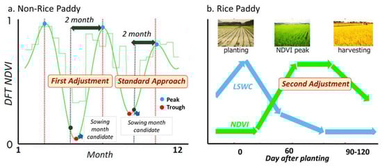
Figure 3.
Three proposed strategies for detecting sowing month in (a) non-rice and (b) rice crop areas.
2.4. Harmonization of Existing Crop Products for Comparison
For cross-validation, we compared the estimated sowing-month and cropping-intensity products with selected existing global products, including MIRCA and SACRA as sowing-month products, and ZABEL (baseline of 1981–2010) as a sowing-month-suitability product. To compare the cropping-intensity product, we used only ZABEL- and SACRA-based products. However, each original dataset has different planting growth units and spatial resolutions. Therefore, for consistency, all the datasets were resampled to one grid of the same level by reproducing comparable datasets with the same resolution, geometry, and unit data. Then, all three cropping-intensity and sowing-month products underwent the harmonization process by reproducing the data at the same level using MODIS-AMSR.
Figure 4 shows the three-level data of the harmonization process with (1) the original product, (2) the reanalyzed product, and (3) the final harmonized product. In this study, we simply used the reanalyzed result of the nearest 30 arc-second grid from the 30 and 5 arc-min grids of MIRCA and SACRA, respectively. We propose a strategy of upscaling the lower resolution without applying the interpolation process to the 1-km pixel resolution. The MODIS-AMSR released the sowing-month product with an aggregate of 1-km pixel resolution.
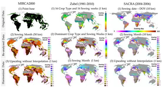
Figure 4.
Three steps for harmonizing the existing crop-calendar product.
3. Results
3.1. MODIS Cropping-Intensity Product
By using the FFT algorithm to analyze the global cropland area, cloud-free NDVI images could be reconstructed for any instant in the temporal sequence. The application of the FFT algorithm to NDVI time-series analysis is an effective means of identifying the vegetation phenology. Figure 5 shows the FFT analysis result of the time-series NDVI data sample in two selected areas in Vietnam (9°44′29.37” N, 106°24′51.85” E) and Thailand (16°44′52.39” N, 100°21′13.18” E). The interpretation of the FFT NDVI phenology shows how the intensity of cropping frequency seems to be changing in these areas. This phenomenon was observed to occur frequently during the 15-year investigation, and the development of irrigation infrastructure can increase the cropping intensity in some cropland areas. Occasional, unpredicted failure to harvest due to disasters may have led to a reduced intensity in some years. Several studies have investigated the increasing and decreasing crop-intensity phenomenon [62,63].
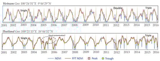
Figure 5.
Original cloud-affected and reconstructed fast Fourier transform (FFT)-based NDVI time series from 2001 to 2015 of locations in Vietnam and Thailand.
Figure 6 shows the result obtained for the average cropping intensity of the dominant crop in the three year groups. For single-cropping intensity, we used the IIASA-IFPRI cropland fraction product. Table 1 shows the estimation results of the cropland areas for single, double, and triple crops at a regional scale. To calculate the areas of single-, double-, and triple-cropping intensities, we converted single-pixel-based products into land-fraction-based products with percentage values ranging from 0% to 100%. The countries where double crops were detected in large areas included the United States (California), Brazil, Uruguay, and Argentina in the Americas; Egypt and Uganda in Africa; the UK and France in Europe; and India, Bangladesh, Thailand, Vietnam, and China in Asia. In addition, countries that dominated specific triple crops included China, Bangladesh, and Vietnam. However, this area estimation shows that there is a big gap between Asia and non-Asian regions regarding the double- and triple-crop agricultural areas.
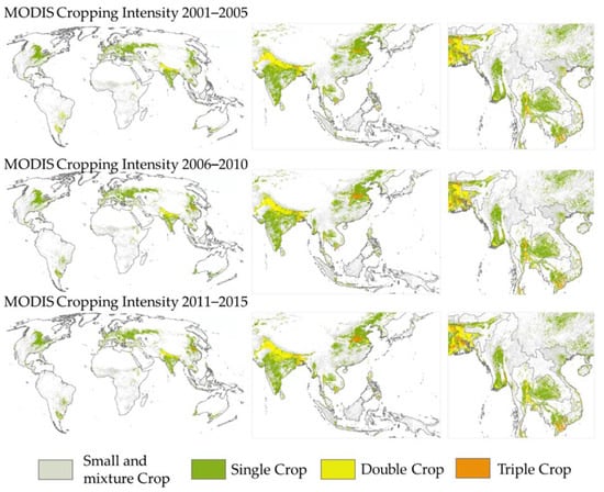
Figure 6.
Global distribution of detected MODIS CI for three year groups: 2001–2005, 2005–2010, and 2011–2015.

Table 1.
The estimation results of the cropland areas for single, double, and triple crops in six regions.
In the global analysis, in 2000–2005, the total double-crop intensity was 7.1 million km2, which increased to 8.3 million km2 in 2006–2010, and then to 8.6 million km2 in 2011–2015. In the same periods, global triple-crop agriculture exhibited a rapid growth of 0.73, 1.12, and 1.28 million km2, respectively. In 2000–2005, the total double-crop growth in Asia was 5.8 million km2, which increased to 5.9 million km2 in 2006–2010, and then rapidly to around 6.5 million km2 in 2011–2015. Moreover, Asia showed an increase of two times for the triple-crop agricultural area over these 15 years, showing a rapid positive growth of 0.65, 1.05, and 1.2 million km2 in 2001–2005, 2006–2010, and 2011–2015, respectively. This indicates how increasing food demand in the Asia region has led to the increased development of irrigation system that have increased the number of cultivation periods in one year [64]. This study also shows how the Africa region has expanded with respect to single-cropping area over these 15 years, with a total growth of 19.02, 19.8, and 21.9 million km2 in 2001–2005, 2006–2010, and 2011–2015, respectively. This shows that Africa is the only region with a growing trend in single-crop agriculture. Although Africa’s growing population has led to an increase in food demand, the development of irrigation infrastructure is still lacking. Given this situation, an “extensification” strategy is more suitable than intensification, which requires more water sources [65]. We calculated the total cropping area by combining the results obtained for single-, double-, and triple-cropping areas and comparing them with the total cropland area using FAO-stat. The comparison of the total crop areas is due to the FAO only addressing the total cropland areas. The comparison shows that the differences between the total cropland areas determined by MODIS CI and FAO-stat are 207,500 km2 in 2001–2005, 243,000 km2 in 2006–2010, and then 252,900 km2 in 2011–2015. Also, the maximum difference among the three groups was 84,300 km2 in Asia, 42,900 km2 in Europe, 31,500 km2 in North America, 55,900 km2 in Africa, 40,000 km2 in South America, and 5000 km2 in Oceania. However, the change trend in the six regions for the three groups exhibited the same pattern, except in South America where the MODIS CI estimate decreased during the 2001–2005 and 2006–2010 periods, while the FAO estimate of the total cropland area increased.
3.2. MODIS-AMSR Sowing-Month Product
The conversion of the unit from day of year (DOY) to month for the detected peaks and troughs can simplify the analysis and provide a stable average sowing schedule. This is also supported by the three aforementioned approaches illustrated in Figure 7 of using (1) standard, (2) first adjustment, and (3) second adjustment products. The target of the first adjustment approach is to investigate the areas with a short cultivation period between sowing and peak months. Central Africa and Northern Russia were detected as possessing large areas of short-cultivated crops. The adjustment strategy can reduce errors, which could be identified by boundary analyses between Bangladesh and India, and showed a contrast difference in the boundary of the two countries, as shown in Figure 8. Further, South Asia and Southeast Asia showed high spatial variation and complexity in the sowing months as water resources were available throughout the year [62,66]. In contrast, the northern regions, such as Europe and the US, have similar climate conditions, and hence their period of cultivation is relatively similar. Some countries, such as Bangladesh, were identified to have a similar sowing month in a major season for almost all areas [67].
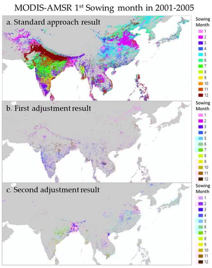
Figure 7.
Global distribution of sowing month result based on (a) the standard approach, (b) first adjustment, and (c) second adjustment in the Asia Pacific region.
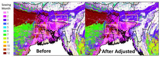
Figure 8.
Comparison of original and adjusted sowing-month products around Bangladesh, India, Nepal, Bhutan, and Myanmar.
The final product of MODIS-AMSR not only provides an estimation of the sowing month in one year but can also be used to conduct a long-term analysis for 15 years, as shown in Figure 9. Information from single-, double-, and triple-cropping grids was used to compute the average sowing date in multiple cropping systems for MODIS-AMSR products. For temporal changes in sowing month, the MODIS-AMSR product considers the effects of human decisions, infrastructure development, changes in season, and natural disasters. In the case of a disaster, such as after a heavy flood, the timing of sowing differs from that of a normal year. Change in sowing month in the three year groups was also found in the case of change in dynamic cropping intensity in areas such as China, India, Bangladesh, and Spain. In the case of Bangladesh, the circled areas in Figure 10 represent areas with a different sowing month among the three year groups as being representative of the sowing-month area due to change in intensity.
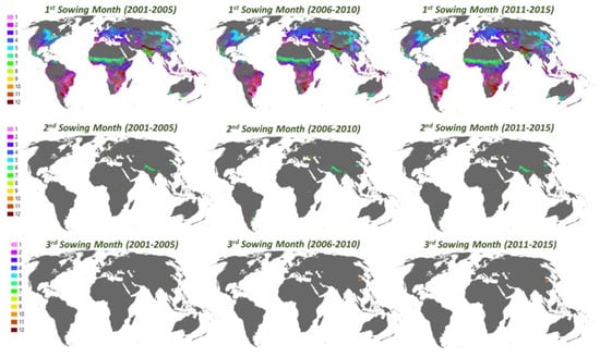
Figure 9.
Sowing-month products for the three year groups 2001–2005, 2006–2010, and 2011–2015.
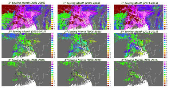
Figure 10.
Fifteen-year sowing-month estimation for the boundary between India and Bangladesh.
To investigate the type of water source in a given cropland area, we used the GFSAD1KCD irrigated and rainfed 1-km datasets [68] and divided the area into irrigated and rainfed regions. Our investigation showed that a sowing-month change area appeared frequently in rainfed areas, such as the southern and eastern parts of India, southern and eastern parts of the United States, and in major cropland areas across Russia. These rainfed crop areas are influenced by annual differences in the timing of the monsoon; these changes impact farmers’ decisions about when to start cultivation. These data were compared with irrigated areas such as the Mekong Delta Vietnam, the northern part of India, and California (US) that had similar patterns of sowing month over the 15-year analysis. These two groups of areas indicate that there are two major driving factors effecting the sowing-month change trends: change in intensity and change in rainy season.
With the integration of MODIS NDVI and AMSR-E/2 LSWC in the second adjustment analysis, we were able to estimate specific sowing months for rice paddy crops. The global paddy-field fractions for 2005, 2010, and 2015, developed using HYDE v3.2, were used to construct a paddy-area base map. To investigate the operation of these VIs and the water index of MODIS-AMSR integration, and to analyze the rice paddy crop, we selected some points located in Bangladesh (Figure 11a). Along with vegetation and water phenology, the changes in the cropping pattern can be used to analyze the rice cropping pattern.
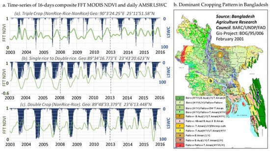
Figure 11.
(a) Integration strategy between time series of 16-day composite FFT MODIS NDVI and daily AMSR LSWC in (b) several cropping-pattern formations in Bangladesh.
The AMSR-based data are useful for monitoring the sowing month because these sensors are all-weather-based and can observe the target area even if the area is covered by cloud [69]. This long-term time-series data analysis was used to monitor agricultural activity over nine years, i.e., 2003–2005, 2008–2010, and 2013–2015. We applied the long-term time-series data analysis to the following three selected cropping patterns: (1) triple crop agriculture: non-rice, rice, non-rice; (2) double crop: rice and rice; and (3) double crop: non-rice and rice. The time-series analysis of MODIS NDVI shows three dominant peaks in each year, while the analysis of AMSR LSWC shows one peak that coincides with the second peak of MODIS NDVI. This cropping pattern indicates three cultivation sessions, in which a rice paddy plantation is part of the second session.
4. Discussion
4.1. Correlation Analysis of Active Crop Intensity and Irrigated Area
As there are no validated data for the single-, double-, and triple-cropping-intensity areas on a global scale, we propose the use of alternative reference data. Active cropping-intensity areas, such as double and triple crops, tend to occur in irrigated areas. For our first visual comparison, we used irrigated HYDE v3.2 because this can provide an irrigated distribution map for a multiyear analysis (Figure 12). The product is developed by a combination of cropland statistical data, satellite information, specific allocation algorithms, and weighting maps. Based on a visual comparison, some countries, such as Thailand, Bangladesh and Vietnam, show a high correlation between the irrigated areas and active cropping-intensity areas. However, not all countries show this tendency; some others such as Myanmar and India show a low correlation between irrigated area and active cropping intensity. This low correlation indicates that the irrigated area still cannot boost food production with increased intensity. This could be because of climate conditions and physical land conditions that complicate attempts to increase the intensity in irrigated areas. This condition follows the fact that not all irrigated areas can produce crops in more than one harvesting period. However, having more than one harvesting period requires more water, which necessitates an irrigation system. Hence, the irrigated area should exhibit a larger area than the total of the double and triple areas.

Figure 12.
Visual comparison between MODIS CI and HYDE 3.2 irrigated area.
Accordingly, in this section, we compare the areas of double and triple crops derived from MODIS CI, SACRA, and ZABEL with irrigated agriculture based on FAO for 2003, 2008, and 2013 as a statistical data reference [31]. The reported irrigation statistics at the national level were obtained from the FAO-Stat database. FAO defines irrigated cropland as the “total area equipped for irrigation” [31]. Figure 13a shows the irrigated areas obtained from FAO-stats and the estimated combination of double and triple areas by MODIS CI at the country level during 2001–2005, 2006–2010, and 2011–2015. The FAO-statistic-based area shows a trend of overestimation compared to the double–triple MODIS CI, with determination coefficients of 0.69, 0.72, and 0.69, respectively. Figure 13b shows the FAO-stats-based irrigated areas and the combination of double and triple areas estimated by the ZABEL and SACRA data at the country level. The FAO-stats-based area shows an underestimation trend compared to the double–triple crop intensity estimated through ZABEL and SACRA, with determination coefficients of 0.37 and 0.34, respectively. The result obtained from the national statistics promotes the MODIS CI product as that with the highest similarity to both irrigated FAO-stats and HYDE irrigated distribution products. The MODIS CI-based double and triple crop areas are the only products that tend to underestimate the FAO-statistic irrigated areas.
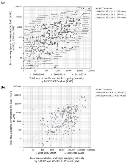
Figure 13.
Comparison of FAO-stats irrigated reported statistics and modeled total double- and triple-cropping areas derived from (a) MODIS CI in three year groups and (b) ZABEL and SACRA cropping-intensity products per country (km2) (N = 162 countries).
4.2. Comparative Analysis of Cropping-Intensity and Sowing-Month Products
High-quality ground data were not available as a reference to validate the results. This unavailability of data makes it difficult to decide which dataset is more accurate for global studies. On the other hand, it is difficult to determine the absolute accuracy of the products through comparison. A high correlation to the FAO statistics is not sufficient to assess the quality of a product. For accurate validation, products with the same or more precise global-level cropland cropping intensity and sowing month should be compared. Because MODIS-AMSR, MIRCA, ZABEL, and SACRA detect cropping intensity and sowing date using different approaches, comparing their results is useful for cross-validation. A comparative analysis between different products can be used as an alternative approach to evaluate the reliability of each product with high consistency. The huge difference can be attributed to different forms of analysis, and the actual reason behind this will be investigated. The different spatial distributions of cropping intensity of products are shown in Figure 14.
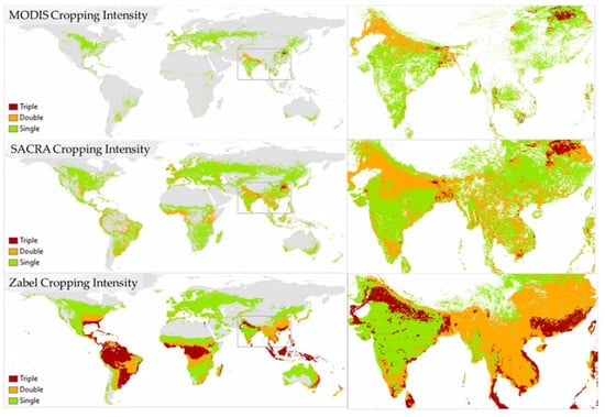
Figure 14.
Comparison of MODIS CI (2006–2010) product with the two previous cropping intensityproducts of SACRA and ZABEL.
With respect to the comparative analysis of cropping intensity, we compared the cropping intensity of the 2001–2005 product obtained using MODIS CI with those of ZABEL and SACRA by using the crisp cross-walk approach of pixel-based agreement analysis [70]. In this intensity comparison, we used only two previous datasets. We did not include MIRCA because the MIRCA product is not directly relevant to cropping intensity, and instead emphasizes data about the five most important crops. These data cannot be directly compared with other products, which have specific information on cropping intensity per year. Agreement analyses are widely used to compare the similarity to various data, and one of the requirements is that the same product level must have comparable data [71]. Because we compare the cropping intensity of three different products in this agreement analysis, we classify the characteristics and group each product into three levels of agreement. Level 1 denotes low agreement, Level 2 denotes medium agreement, and Level 3 denotes high agreement. Figure 13a,b shows the agreement analysis result between MODIS CI, SACRA, and ZABEL for double and triple crops. With respect to double cropping, Pakistan, Egypt, Bangladesh, and North India are the top four areas that have high agreement among the three copping-intensity datasets (Figure 15). With respect to triple cropping, some parts of China and Bangladesh show agreement and are identified as Level 2.
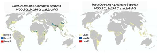
Figure 15.
Agreement analysis between MODIS CI, SACRA CI, and ZABEL CI products for double-cropping area (left) and triple-cropping area (right).
To analyze the distribution of agreement levels, Table 2 lists a comparison of three agreement levels for three cropping-intensity products (MODIS CI, SACRA, and ZABEL) in double- and triple-cropping areas. As shown, SACRA and ZABEL identified double intensity at 76% and 98.5%, respectively, in Level 1; this indicates that SACRA and ZABEL overestimate double-cropping intensity. For example, some areas that are unsuitable for double cropping due to low irrigation infrastructure and low precipitation were detected to have double-cropping intensity, such as the Africa region. The MODIS CI product dominates in Level 2 and Level 3 for double cropping (83.1%) and for triple cropping (64.4%). Based on the distribution of the Level 2 and Level 3 agreement, MODIS CI exhibits a higher number of reliable product dominant pixels that are located in the higher agreement levels of Level 2 and Level 3.
Table 2.
Percentage of the total number of pixels for each cropping-intensity product in three levels of double- and triple-cropping agreement.
A comparative analysis was also proposed for the sowing-month products of MODIS-AMSR, MIRCA, SACRA, and ZABEL. Figure 16 shows a visual comparison of the four harmonized sowing-month products for the southern and south-east parts of Asia. A comparison between the MODIS-AMSR product and the harmonized products of MIRCA, SACRA, and ZABEL for sowing-month products is shown in Figure 17. The comparison product has to be converted by cycling mode to simplify it for the different analyses of sowing month. Without cycling mode, the difference between the two sowing-month products can range from −11 to +11 (11 months earlier or 11 months later). After cycling mode, the difference between the two sowing-month products can be 0–6. This indicates that the sowing month differs in each pixel by 0 months (same month) to 6 months. Figure 16 shows the differences between the sowing-month products for MODIS-AMSR and the three previous sowing-month datasets, namely, MIRCA, ZABEL, and SACRA. The results show that the sowing-month product obtained through SACRA has the highest similarity to that obtained by MODIS-AMSR, where SACRA and ZABEL show different dominant pixel numbers in one month. The difference between the estimated sowing month and other existing products, especially for SACRA and ZABEL, is less than 2 months for more than 60% of the areas (Figure 17). A comparison of three adjustment levels of the MODIS-AMSR sowing-month product, i.e., the standard approach, first adjustment, and second adjustment, with the three existing datasets of SACRA, ZABEL, and SACRA was conducted to evaluate the performance improvement. By implementing a first and second adjustment for estimating the sowing-month product in MODIS-AMSR, we can reduce the 6-month difference in the comparison analysis for both SACRA and ZABEL products (Figure 17).
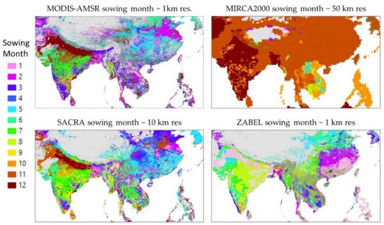
Figure 16.
Comparison of the MODIS-AMSR sowing-month (2006–2010) product with the three previous sowing-month products of MIRCA, SACRA, and ZABEL.
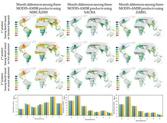
Figure 17.
Month differences between three MODIS-AMSR sowing-month products for MIRCA (left), SACRA (center), and ZABEL (right). Only single-cropping grids are used to compute the compared sowing date.
The same sowing month (0 month difference) between MODIS-AMSR and MIRCA is found for around 3 million pixels, becoming around 7.5 million for ZABEL and 11.5 million for SACRA. MODIS-AMSR has the highest similarity to SACRA, followed by ZABEL and MIRCA. Huge differences in more than 3 months were found between MODIS-AMSR and MIRCA products, where the difference between 5 months was considered to be the highest pixel number. Considering the extreme disagreement between MODIS-AMSR and the three existing datasets in some regions, it is important to determine which sowing month is more reliable. These regions are found in the northern part of Russia, the southern part of China, and the eastern part of India. Low-agreement datasets between MODIS-AMSR and previous sowing-month products were observed for regions predominantly located in rainfed areas, where the climate influence is greater.
4.3. Uncertainties in Cropping Intensity and Sowing Month
A comparison of the census-based product MIRCA, the model-based product ZABEL, and the satellite-model-based product SACRA shows that there are still large differences between these products. Differences in pixel resolution, input data, and type of method make it difficult to achieve a high global cropping intensity, and sowing month estimation becomes challenging. The accuracy of MODIS-AMSR depends on the accuracy of the MODIS NDVI and AMSR LSWC datasets. It is difficult to demonstrate global variability without knowledge of the local sowing months. For a local investigation, we highlighted a comparison of two countries: Bangladesh and Japan. The products of cropping intensity and sowing month of these two countries were compared with the United States Department of Agriculture (USDA) crop calendar [72]. The product crop calendar derived from the USDA shows the top five crop types in both countries. In Bangladesh, the top five dominant crops are rice (Aman), rice (Aus), rice (Boro), sorghum, and wheat (Figure 11b), and the dominant sowing months are January, March, and December. In Japan, the top five crops are barley, rice (central-south), rice (north, Hokkaido), soybeans, and wheat, and the dominant sowing months are April, May, and June. If the results are compared using visual MODIS-AMSR, the sowing-month products in Bangladesh are similar to the results of the USDA crop calendar. However, in the case of Japan, MODIS-AMSR products are not only detected in April, May, and June but are also detected in December and January in some pixels. This difference reflects the complexity of detecting sowing months in a pixel-based analysis. For countries with large irrigation areas such as India, Vietnam, the US, and China, high sowing-month agreement (with 0–2 month differences) is mostly found in the irrigated areas. However, countries with small irrigated areas such as Argentina, the UK, Russia, and South Africa, high and low sowing-month agreements are randomly distributed in both the irrigated and rainfed areas.
A mixture of several crops in a grid is not considered in this study, as it was assumed that the dominant crop is derived from an agricultural field with a 1-km pixel resolution for the cropping-intensity and sowing-month products; this could be false and could be a major source of discrepancy in distinguishing crop type [73]. We assume that the time series of NDVI and LSWC represent the phenology of one dominant crop, and thus we estimate the intensity and sowing month of the dominant crop in each grid. A major discrepancy in crop calendars between MODIS-AMSR and other products (MIRCA, ZABEL, and SACRA) may occur due to the selection of one dominant crop in each pixel unit. The disadvantages of this approach may be reduced by including finer satellite sensors in the development algorithm, such as Landsat, Sentinel, or Global Change Observation Mission–Climate (GCOM-C), to avoid mixtures of phenologies. Some studies have attempted to increase the resolution of AMSR-E by blending the data with MODIS [74]. These include crop-type classification studies that have considered several dominant crops in each grid. For a specific rice paddy area, by comparing the sowing-month product with RiceAtlas [75], a rice paddy crop-calendar product derived from census data should also be investigated.
Another limitation of the product is the saturation effect on NDVI data owing to red band absorption in the NDVI formula. The pigments which are absorbers are material density causing refractions that lead to multi scattering. Further improvements and enhanced techniques are required to address the NDVI saturation problem, such as the Wide Dynamic Range Vegetation Index (WDRVI) [76] and saturation-adjusted NDVI [77]. Another method is to implement other indexes such as the Enhanced Vegetation Index (EVI) [78], which was designed for highly dense vegetation cover and is capable of addressing saturation issues. Other factors such as cloud contamination problems that have been addressed by several studies [79] have not been considered in this study. Cloud contamination prevents us from acquiring cropping frequency, even when 5-year MODIS NDVI products are used. Especially in a tropical area, the amount of cloud is higher than that of other areas, and this may be a source of discrepancy in the analysis.
Some studies have integrated various crop type datasets with models considering that each crop type has a different characteristic, especially for the crop growth period. Further validation, including the distribution in global areas by a camera field survey or an automatic weather station (AWS), is required for ensuring crop phenology, especially where crops are considerably complicated. Accurate validation is required to compare the product with a more precise country-level cropping-intensity area that has a higher resolution. Globland30 [80] and the Unified Cropland layer [81] may be used as alternatives for validation analysis in future studies.
4.4. Future Possible Directions
Future applications with environmental and socio-economic implications could be explored. Improved cropping intensity and sowing month would enhance our ability to measure crop production and improve crop management [82]. The impact of this change on environmental health, including in forests [83,84,85], urban areas [86,87], and surface water or rivers [88], could also be explored. Further investigations are required to elucidate the reason for this sowing month change, the impact of this change on the food security situation, and future projections. Improving the irrigation infrastructure in intensively cultivated areas can help to address water loss problems. This is because the highest water demands are located in the irrigation sector and are also the biggest contributor to global water wastage problems [20]. The improvement of intensity and sowing month estimation could also improve water management strategies such as agricultural drainage water (ADW) in rice paddies [89]. This strategy has great near-term potential to reduce GHG emission intensity without affecting food production. Integration remote sensing by combining a projection model with a simulated global climate model could be an alternative option to improve future crop conditions. The impacts of intensity and cultivation changes on socio-economic parameters at country and sub-country levels must also be analyzed. Gridded global datasets for Gross Domestic Product [90] combined with the Development Flows to Agriculture (DFA) and Gross Fixed Capital Formation (GFCF) could be used as an alternative way to investigate the relationship between investment and crop production [91]. By improving data, a new strategy to increase food production and reduce water crises due to high irrigation water demands (such as the study on redistribution of cropland areas in [23]) could be more accurately proposed.
5. Conclusions
In this study, we developed a 1-km long-term analysis of cropping intensity and sowing month in three groups of years by using integration time-series MODIS NDVI and AMSR-E/2 LSWC datasets. FFT was applied to time series of MODIS NDVI data, and it was found that crop intensity was well modeled for single, double, and triple crops. The cultivation period is identified from the time series of NDVI and LSWC, which correspond to vegetation vitality and water surface. Satellite-sensed NDVI and LSWC data enable the detection of whether the managed land is currently cultivated or temporarily in disuse. The improvement of the developed algorithm, considering the short period of cultivation as well as the flooding session by surface water coverage from AMSR-E/2, may be useful. The FAO-statistic-based area shows a trend of overestimation compared to the double–triple MODIS CI, with determination coefficients of 0.69, 0.72, and 0.69 in the three groups of years. The MODIS CI product dominates in the agreement levels of Level 2 and Level 3 for double cropping (83.1%) and for triple cropping (64.4%). Based on the agreement level analysis, MODIS CI exhibits a higher number of reliable product dominant pixels that are located in the higher agreement levels of Level 2 and Level 3. The difference between the estimated sowing month and other existing products, especially for SACRA and ZABEL, is less than 2 months for more than 60% of the areas. Implementing a first and second adjustment for estimating the sowing-month product in MODIS-AMSR can reduce the 6-month difference in the comparison analysis for both SACRA and ZABEL products. The finer spatial resolution combined with long-term global analysis products allows it to be applied in several sustainability studies, from global- to local-level perspectives.
Author Contributions
A.D.S. conceived and designed the experiments; A.D.S. and W.T. performed the experiments; A.D.S. analyzed the data; A.D.S., and W.T. preprocessed the base datasets; A.D.S. wrote the paper; and all authors read the paper and provided revision suggestions. All authors have read and agreed to the published version of the manuscript.
Funding
This project was funded by Research, Community Service and Innovation Program provided by Institut Teknologi Bandung, Kurita Asia Research Grant (19Pid017) provided by Kurita Water and Environment Foundation, and MIRA program of the Ministry of Research and Higher Education of Indonesia.
Acknowledgments
The authors gratefully acknowledge support from the Global Leader Program for Social Design and Management by the Ministry of Education, Culture, Sport, Science and Technology Japan, Kurita Water and Environment Foundation, MIRA program of the Ministry of Research and Higher Education of Indonesia and Institut Teknologi Bandung. We also thank the anonymous reviewers whose valuable comments greatly helped us to prepare an improved and clearer version of this paper. All persons and institutes who kindly made their data available for this analysis are acknowledged.
Conflicts of Interest
The authors declare no conflict of interest.
References
- Loewenberg, S. Global food crisis looks set to continue. Lancet 2008, 372, 1209–1210. [Google Scholar] [CrossRef]
- Godfray, H.C.J.; Beddington, J.R.; Crute, I.R.; Haddad, L.; Lawrence, D.; Muir, J.F.; Pretty, J.; Robinson, S.; Thomas, S.M.; Toulmin, C. Food security: The challenge of feeding 9 billion people. Science 2010, 327, 812–818. [Google Scholar] [CrossRef]
- Imadi, S.R.; Shazadi, K.; Gul, A.; Hakeem, K.R. Sustainable Crop Production System. In Plant Soil and Microbes; Hakeem, K.R., Akhtar, M.S., Abdullah, S.N.A., Eds.; Springer International Publishing: Cham, Switzerland, 2016. [Google Scholar]
- Lewandowski, I.; Hardtlein, M.; Kaltschmitt, M. Sustainable Crop Production: Definition and Methodological Approach for Assessing and Implementing Sustainability. Crop Sci. 1999, 39, 184–193. [Google Scholar] [CrossRef]
- UN DESA. World Population Prospects: The 2015 Revision; United Nation: New York, NY, USA, 2015.
- Bruinsma, J. The Resources Outlook: By How Much Do Land, Water and Crop Yields Need to Increase by 2050? Looking Ahead in World Food and Agriculture: Perspectives to 2050; FAO: Rome, Italy, 2011. [Google Scholar]
- Wolffa, S.; Schrammeijera, E.A.; Schulp, C.J.E.; Verburga, P.H. Meeting global land restoration and protection targets: What would the world look like in 2050? Glob. Environ. Chang. 2018, 52, 259–272. [Google Scholar] [CrossRef]
- Seto, K.C.; Güneralp, B.; Hutyra, L.R. Global forecasts of urban expansion to 2030 and direct impacts on biodiversity and carbon pools. Proc. Natl. Acad. Sci. USA 2012, 109, 16083–16088. [Google Scholar] [CrossRef] [PubMed]
- Avellan, T.; Meier, J.; Mauser, W. Are urban areas endangering the availability of rainfed crop suitable land? Remote Sens. Lett. 2012, 3, 631–638. [Google Scholar] [CrossRef]
- Heino, M.; Puma, M.J.; Ward, P.J.; Gerten, D.; Heck, V.; Siebert, S.; Kummu, M. Two-thirds of global cropland area impacted by climate oscillations. Nat. Commun. 2018, 9, 1257. [Google Scholar] [CrossRef]
- Wu, W.; Yua, Q.; Youb, L.; Chenb, K. Global cropping intensity gaps: Increasing food production without cropland expansion. Land Use Policy 2018, 2, 32. [Google Scholar] [CrossRef]
- Siebert, S.; Portmann, F.T.; Döll, P. Global patterns of cropland use intensity. Remote Sens. 2010, 2, 1625–1643. [Google Scholar] [CrossRef]
- FAO; IFAD; WFP. The State of Food Insecurity in the World 2013. The Multiple Dimensions of food Security; FAO: Rome, Italy, 2013. [Google Scholar]
- Delzeit, R.; Lewandowski, I.; Arslan, A.; Cadisch, G.; Erisman, J.W.; Ewert, F.; Klein, A.M.; von Haaren, C.; Lotze-Campen, H.; Mauser, W.; et al. How the Sustainable Intensification of Agriculture can Contribute to the Sustainable Development Goals? Working Paper; German Committee Future Earth: Stuttgart, Germany, 2018; Volume 18, p. 1. [Google Scholar]
- Rufin, P.; Levers, C.; Baumann, M.; Jägermeyr, J.; Krueger, T.; Kuemmerle, T.; Hostert, P. Global-scale patterns and determinants of cropping frequency in irrigation dam command areas. Glob. Environ. Chang. 2018, 50, 110–122. [Google Scholar] [CrossRef]
- Bondeau, A.; Smith, P.C.; Zaehle, S.; Schaphoff, S.; Lucht, W.; Cramer, W.; Gerten, D.; Lotze-Campen, H.; Müller, C.; Reichstein, M.; et al. Modelling the role of agriculture for the 20th century global terrestrial carbon balance. Glob. Chang. Biol. 2007, 13, 679–706. [Google Scholar] [CrossRef]
- See, L.M.; Fritz, S.; You, L.; Ramankutty, N.; Herrero, M.; Justice, C.; Becker-Reshef, I.; Thornton, P.; Erb, Z.; Gong, P.; et al. Improved global cropland data as an essential ingredient for food security. Glob. Food Secur. 2014, 4, 37–45. [Google Scholar] [CrossRef]
- ESA. Satellite Earth Observations in Support of the Sustainable Development Goals, 3rd ed.; Special 2018 Edition; CEOS: Paris, France, 2018.
- Ray, D.K.; Mueller, N.D.; West, P.C.; Foley, J.A. Yield Trends Are Insufficient to Double Global Crop Production by 2050. PLoS ONE 2013, 8, e66428. [Google Scholar] [CrossRef] [PubMed]
- Döll, P.; Siebert, S. Global modeling of irrigation water requirements. Water Resour. Res. 2002, 38, 8. [Google Scholar] [CrossRef]
- Wada, Y.; Beek, L.P.H.; Viviroli, D.; Dürr, H.H.; Weingartner, R.; Bierkens, M.F.P. Global monthly water stress: II. Water demand and severity of water. Water Resour. Res. 2011, 47, 7. [Google Scholar] [CrossRef]
- Oki, T.; Kanae, S. Global Hydrological Cycles and World Water Resources. Science 2006, 313, 1068–1072. [Google Scholar] [CrossRef]
- Davis, K.F.; Rulli, M.C.; Seveso, A.; D’odorico, P. Increased food production and reduced water use through optimized crop distribution. Nat. Geosci. 2017, 10, 12. [Google Scholar] [CrossRef]
- Portmann, F.T.; Siebert, S.; Döll, P. MIRCA2000—Global monthly irrigated and rainfed crop areas around the year 2000: A new high-resolution data set for agricultural and hydrological modeling. Glob. Biogeochem. Cycles 2010, 24, 1–24. [Google Scholar] [CrossRef]
- Frolking, S.; Qiu, J.; Boles, S.; Xiao, X.; Liu, J.; Zhuang, Y.; Li, C.; Qin, X. Combining remote sensing and ground census data to developnew maps of the distribution of rice agriculture in China. Glob. Biogeochem. Cycles 2002, 16, 1091. [Google Scholar] [CrossRef]
- Monfreda, C.; Ramankutty, N.; Foley, J.A. Farming the planet: 2. Geographic distribution of crop areas, yields, physiological types, and net primary production in the year 2000. Glob. Biogeochem. Cycles 2008, 22, 1. [Google Scholar] [CrossRef]
- Waha, K.; Van Bussel, L.G.J.; Müller, C. Climate-driven simulation of global crop sowing dates. Glob. Ecol. Biogeogr. 2012, 21, 247–259. [Google Scholar] [CrossRef]
- Zabel, F.; Putzenlechner, B.; Mauser, W. Global Agricultural Land Resources. A High Resolution Suitability Evaluation and Its Perspectives until 2100 under Climate Change Conditions. PLoS ONE 2014, 9, e107522. [Google Scholar] [CrossRef]
- Tao, F.; Yokozawa, M.; Zhang, Z. Modelling the impacts of weather and climate variability on crop productivity over a large area: A new process-based model development, optimization, and uncertainties analysis. Agric. For. Meteorol. 2009, 149, 831–850. [Google Scholar] [CrossRef]
- Porter, J.R.; Semenov, M.A. Crop response to climatic variation. Philos. Trans. R. Soc. B Biol. Sci. 2005, 360, 2021–2035. [Google Scholar] [CrossRef] [PubMed]
- Lizumi, T.; Ramankutty, N. How do weather and climate influence cropping area and intensity. Glob. Food Secur. 2015, 4, 46–50. [Google Scholar]
- Lizumi, T.; Kim, W.; Nishimori, M. Modeling the global sowing and harvesting windows of major crops around the year 2000. J. Adv. Model. Earth Syst. 2019, 11, 99–112. [Google Scholar]
- Joshi, N.; Baumann, M.; Ehammer, A.; Fensholt, R.; Grogan, K.; Hostert, P.; Jepsen, M.R.; Kuemmerle, T.; Meyfroidt, P.; Mitchard, E.T.A.; et al. A Review of the Application of Optical and Radar Remote Sensing Data Fusion to Land Use Mapping and Monitoring. Remote Sens. 2016, 8, 70. [Google Scholar] [CrossRef]
- Dong, J.; Zhuang, D.F.; Huang, Y.H.; Fu, J.Y. Advances in multi-sensor data fusion: Algorithms and applications. Sensors 2009, 9, 7771–7784. [Google Scholar] [CrossRef]
- Gu, Y.; Brown, J.F.; Miura, T.; van Leeuwen, W.J.D.; Reed, B.C. Phenological classification of the United States: A geographic framework for extending multi-sensor time-series data. Remote Sens. 2010, 2, 526–544. [Google Scholar] [CrossRef]
- Kotsuki, S.; Tanaka, K. SACRA—A method for the estimation of global high-resolution crop calendars from a satellite-sensed NDVI. Hydrol. Earth Syst. Sci. 2015, 19, 4441–4461. [Google Scholar] [CrossRef]
- Hanasaki, N.; Yoshikawa, S.; Kakinuma, K.; Kanae, S. A seawater desalination scheme for global hydrological models. Hydrol. Earth Syst. Sci. 2016, 20, 4143–4157. [Google Scholar] [CrossRef]
- FAOSTAT. FAOSTAT Database; Food and Agriculture Organization of the United Nations: Rome, Italy, 2016; Available online: http://www.fao.org/faostat/en/#data/QC (accessed on 2 January 2019).
- Goldewijk, K.K.; Beusen, A.; Doelman, J.; Stehfest, E. Anthropogenic land use estimates for the Holocene—HYDE 3.2. Earth Syst. Sci. Data 2017, 9, 927–953. [Google Scholar] [CrossRef]
- Zhang, X.; Friedl, M.A.; Schaaf, C.B.; Strahler, A.H.; Hodges, J.C.F.; Gao, F.; Reed, B.C.; Huete, A. Monitoring vegetation phenology using MODIS. Remote Sens. Environ. 2003, 84, 471–475. [Google Scholar] [CrossRef]
- Pittman, K.; Hansen, M.C.; Beckerreshef, I.; Potapov, P.; Justice, C.O. Estimating global cropland extent with multi-year MODIS data. Remote Sens. 2010, 2, 1844–1863. [Google Scholar] [CrossRef]
- Gray, J.; Friedl, M.A.; Frolking, S.; Ramankutty, N.; Nelson, A.; Gumma, M.K. Mapping Asian Cropping Intensity with MODIS. IEEE J. Sel. Top. Appl. Earth Obs. Remote Sens. 2014, 7, 3373–3379. [Google Scholar] [CrossRef]
- Estel, S.; Kuemmerle, T.; Levers, C.; Baumann, M.; Hostert, P. Mapping cropland-use intensity across Europe using MODIS NDVI time series. Environ. Res. Lett. 2016, 11, 024015. [Google Scholar] [CrossRef]
- Tatsumi, K. Cropping Intensity and seasonality parameters across Asia extracted by multi-temporal SPOT vegetation data. J. Agric. Meteorol. 2016, 72, 142–150. [Google Scholar] [CrossRef]
- Sakamoto, T.; Yokozawa, M.; Toritani, H.; Shibayama, M.; Ishitsuka, N.; Ohono, H. A crop phenology detection method using time-series MODIS data. Remote Sens. Environ. 2005, 96, 366–374. [Google Scholar] [CrossRef]
- Pettorelli, N.; Vik, J.O.; Mysterud, A.; Gaillard, J.M.; Tucker, C.J.; Stenseth, N.C. Using the satellite-derived NDVI to assess ecological responses to environmental change. Trends Ecol. Evol. 2005, 20, 503–510. [Google Scholar] [CrossRef]
- Kawanishi, T.; Sezai, T.; Ito, Y.; Imaoka, K.; Takeshima, T.; Ishido, Y.; Shibata, A.; Miura, M.; Inahata, H.; Spencer, R.W. The Advanced Microwave Scanning Radiometer for the Earth Observing System (AMSR-E), NASDA’s contribution to the EOS for global energy and water cycle studies. IEEE Trans. Geosci. Remote Sens. 2003, 41, 184–194. [Google Scholar] [CrossRef]
- Imaoka, K.; Sezai, T.; Takeshima, T.; Kawanishi, T.; Shibata, A. Instrument characteristics and calibration of AMSR and AMSR-E. In Proceedings of the IEEE International Geoscience and Remote Sensing Symposium, Toronto, ON, Canada, 24–28 June 2002; Volume 1, pp. 18–20. [Google Scholar]
- Takeuchi, W.; Gonzalez, L. Blending MODIS and AMSR-E to predict daily land surface water coverage. In Proceedings of the International Remote Sensing Symposium (ISRS), Busan, Korea, 28–30 October 2009. [Google Scholar]
- Takeuchi, W.; Komori, D.; Oki, T.; Yasuoka, Y. An integrated approach on rice paddy irrigation pattern monitoring over Asia with MODIS and AMSR-E. In Proceedings of the American Geophysical Union Fall Meeting (AGU), San Francisco, CA, USA, 7–11 December 2006. [Google Scholar]
- Arai, H.; Takeuchi, W.; Oyoshi, K.; Nguyen, L.D.; Inubushi, K. Estimation of Methane Emissions from Rice Paddies in the Mekong Delta Based on Land Surface Dynamics Characterization with Remote Sensing. Remote Sens. 2018, 10, 1438. [Google Scholar] [CrossRef]
- Li, X.; Takeuchi, W. Land Surface Water Coverage Estimation with PALSAR and AMSR-E for Large Scale Flooding Detection. Terr. Atmos. Ocean. Sci. 2016, 27, 473–480. [Google Scholar] [CrossRef]
- Roerink, G.J.; Menenti, M.; Verhoef, W. Reconstructing cloud free NDVI composites using Fourier analysis of time series. Int. J. Remote Sens. 2000, 21, 1911–1917. [Google Scholar] [CrossRef]
- Juarez, R.I.N.; Liu, W.T. FFT Analysis on NDVI Annual Cycle and Climatic Regionality in Northeast Brazil. Int. J. Climatol. 2001, 21, 1803–1820. [Google Scholar] [CrossRef]
- Zhang, M.; Zhou, Q.; Chen, Z.; Jia, L.; Yong, Z.; Cai, C. Crop discrimination in Northern China with double cropping systems using Fourier analysis of time-series MODIS data. Int. J. Appl. Earth Obs. Geoinf. 2008, 10, 476–485. [Google Scholar]
- Galford, G.L.; Mustard, J.F.; Melillo, J.; Gendrin, A.; Cerri, C.C.; Cerri, E.P. Wavelet analysis of MODIS time series to detect expansion and intensification of row-crop agriculture in Brazil. Remote Sens. Environ. 2008, 112, 576–587. [Google Scholar] [CrossRef]
- Fritz, S.; See, L.; Mccallum, I.; You, L.; Bun, A.; Moltchanova, E.; Duerauer, M.; Albrecht, F.; Schill, C.; Perger, C.; et al. Mapping global cropland and field size. Glob. Chang. Biol. 2015, 21, 1980–1992. [Google Scholar] [CrossRef]
- Rocchini, D.; Metz, M.; Ricotta, C.; Landa, M.; Frigeri, A.; Neteler, M. Fourier transforms for detecting multitemporal landscape fragmentation by remote sensing. Int. J. Remote Sens. 2013, 34, 8907–8916. [Google Scholar] [CrossRef]
- Negri, L.H.; Vestri, C. Peakutils: v1.1.0. 2017. Available online: https://doi.org/10.5281/zenodo.887917 (accessed on 2 October 2019).
- FAO. CROPWAT 8 User Guide: A Computer Program for Irrigation Planning and Management; Food and Agriculture Organization of the United Nations: Rome, Italy, 2009. [Google Scholar]
- Sacks, W.J.; Deryng, D.; Foley, J.A.; Ramankutty, N. Crop planting dates: An analysis of global patterns. Glob. Ecol. Biogeogr. 2010, 19, 607–620. [Google Scholar] [CrossRef]
- Jiang, M.; Xin, L.; Li, X.; Tan, M.; Wang, R. Decreasing Rice Cropping Intensity in Southern China from 1990 to 2015. Remote Sens. 2018, 11, 35. [Google Scholar] [CrossRef]
- Chen, B. Globally Increased Crop Growth and Cropping Intensity from the Long-term Satellite-Based Observation. In ISPRS Annals of the Photogrammetry, Remote Sensing and Spatial Information Sciences; Copernicus Publications: Göttingen, Germany, 2018; Volume IV-3. [Google Scholar]
- Biradar, C.M.; Xiao, X. Quantifying the area and spatial distribution of double-and triple-cropping croplands in India with multi-temporal MODIS imagery in 2005. Int. J. Remote Sens. 2011, 32, 367–386. [Google Scholar] [CrossRef]
- Tadele, Z. Raising Crop Productivity in Africa through Intensification. Agronomy 2017, 7, 22. [Google Scholar] [CrossRef]
- Lasko, K.; Vadrevu, K.P.; Tran, V.T.; Justice, C. Mapping Double and Single Crop Paddy Rice with Sentinel-1A at Varying Spatial Scales and Polarizations in Hanoi, Vietnam. IEEE J. Sel. Top. Appl. Earth Obs. Remote Sens. 2018, 11, 498–512. [Google Scholar] [CrossRef] [PubMed]
- Nasim, M.; Shahidullah, S.M.; Saha, A.; Muttaleb, M.A.; Aditya, T.L.; Ali, M.A.; Kabir, M.S. Distribution of Crops and Cropping Patterns in Bangladesh. Bangladesh Rice J. 2017, 21, 1–55. [Google Scholar] [CrossRef]
- Thenkabail, P.; Knox, J.; Ozdogan, M.; Gumma, M.; Congalton, R.; Wu, Z.; Milesi, C.; Finkral, A.; Marshall, M.; Mariotto, I.; et al. NASA Making Earth System Data Records for Use in Research Environments (MEaSUREs) Global Food Security Support Analysis Data (GFSAD) Crop Dominance 2010 Global 1 km V001; NASA EOSDIS Land Processes DAAC: Sioux Falls, SD, USA, 2016.
- Shibata, A.; Imaoka, K.; Koike, T. AMSR/AMSR-E level 2 and 3 algorithm developments and data validation plans of NASDA. IEEE Trans. Geosci. Remote Sens. 2003, 41, 195–203. [Google Scholar] [CrossRef]
- Bai, Y.; Feng, M.; Jiang, H.; Wang, J.; Zhu, Y.; Liu, Y. Assessing Consistency of Five Global Land Cover Data Sets in China. Remote Sens. 2014, 6, 8739–8759. [Google Scholar] [CrossRef]
- Sakti, A.D.; Takeuchi, W.; Wikantika, K. Development of Global Cropland Agreement Level Analysis by Integrating Pixel Similarity of Recent Global Land Cover Datasets. J. Environ. Prot. 2017, 8, 1509–1529. [Google Scholar] [CrossRef][Green Version]
- USDA. Agricultural Statistics Service, 2002 Census of Agriculture; Geographic Area Series, Part 51; United States Summary and State Data: Washington, DC, USA, 2004; Volume 1.
- Ozdogan, M. The spatial distribution of crop types from MODIS data: Temporal unmixing using Independent Component Analysis. Remote Sens. Environ. 2010, 114, 1190–1204. [Google Scholar] [CrossRef]
- Takeuchi, W.; Yongjoo, K. Blending MODIS and AMSR2 to predict daily global inundation map in 1 km resolution. In Proceedings of the 2018 IEEE International Geoscience and Remote Sensing Symposium, Valencia, Spain, 22–27 July 2018. [Google Scholar]
- Laborte, A.G.; Gutierrez, M.A.; Balanza, J.G.; Saito, K. RiceAtlas, a spatial database of global rice calendars and production. Sci. Data 2017, 4, 170074. [Google Scholar] [CrossRef]
- Gitelson, A.A. Wide Dynamic Range Vegetation Index for remote quantification of biophysical characteristics of vegetation. J. Plant Physiol. 2004, 161, 165–173. [Google Scholar] [CrossRef]
- Gu, Y.; Wylie, B.K.; Howard, D.M.; Phuyal, K.P.; Ji, L. NDVI saturation adjustment: A new approach for improving cropland performance estimates in the Greater Platte River Basin, USA. Ecol. Indic. 2012, 30, 1–6. [Google Scholar] [CrossRef]
- Liu, H.Q.; Huete, A.R. A feedback based modification of the NDV I to minimize canopy background and atmospheric noise. IEEE Trans. Geosci. Remote Sens. 1995, 33, 457–465. [Google Scholar] [CrossRef]
- Ozdogan, M.; Woodcock, C.E. Resolution dependent errors in remote sensing of cultivated areas. Remote Sens. Environ. 2006, 103, 203–217. [Google Scholar] [CrossRef]
- Chen, J.; Liao, A.; Cao, X.; Chen, L.; Chen, X.; He, C.; Han, G.; Peng, S.; Lu, M.; Zhang, W.; et al. Global land cover mapping at 30 m resolution: A POK-based operational approach. ISPRS J. Photogramm. Remote Sens. 2015, 103, 7–27. [Google Scholar] [CrossRef]
- Waldner, F.; Fritz, S.; Di Gregorio, A.; Plotnikov, D.; Bartalev, S.; Kussul, N.; Gong, P.; Thenkabail, P.; Hazeu, G.; Klein, I.; et al. A Unified Cropland Layer at 250 m for Global Agriculture Monitoring. Data 2016, 1, 3. [Google Scholar] [CrossRef]
- Romaguera, M.; Hoekstra, A.Y.; Su, Z.; Krol, M.S.; Salam, M.S. Potential of Using Remote Sensing Techniques for Global Assessment of Water Footprint of Crops. Remote Sens. 2010, 2, 1177–1196. [Google Scholar] [CrossRef]
- Sakti, A.D.; Tsuyuki, S. Spectral Mixture Analysis of Peatland Imagery for Land Cover Study of Highly Degraded Peatland in Indonesia. In The International Archives of the Photogrammetry, Remote Sensing and Spatial Information Science; Copernicus Publications: Göttingen, Germany, 2015; Volume XL-7/W3. [Google Scholar]
- Lawrence, D.; Radel, C.; Tully, K.; Schmook, B.; Schneider, L. Untangling a decline in tropical forest resilience: Constraints on the sustainability of shifting cultivation across the globe. Biotropica 2010, 42, 21–30. [Google Scholar] [CrossRef]
- Fauzi, A.; Sakti, A.; Yayusman, L.; Harto, A.; Prasetyo, L.; Irawan, B.; Kamal, M.; Wikantika, K. Contextualizing Mangrove Forest Deforestation in Southeast Asia Using Environtmental and Socio-Economic Data Product. Forest 2019, 10, 952. [Google Scholar] [CrossRef]
- Bren d’Amour, C.; Reitsma, F.; Baiocchi, G.; Barthel, S.; Güneralp, B.; Erb, K.; Haberl, H.; Creutzig, F.; Seto, K.C. Future urban land expansion and implications for global croplands. Proc. Natl. Acad. Sci. USA 2017, 114, 8939–8944. [Google Scholar] [CrossRef]
- Ramankutty, N.; Mehrabi, Z.; Waha, K. Trends in Global Agricultural Land Use: Implications for Environmental Health and Food Security. Annu. Rev. Plant Biol. 2018, 69, 1–14. [Google Scholar] [CrossRef] [PubMed]
- Barbarossa, V.; Huijbregts, M.A.J.; Beusen, A.H.W.; Beck, H.E.; King, H.; Schipper, A.M. FLO1K, global maps of mean, maximum and minimum annual streamflow at 1 km resolution from 1960 through 2015. Sci. Data 2018, 5, 180052. [Google Scholar] [CrossRef] [PubMed]
- Tanji, K.K. Agricultural Drainage Water Management in Arid and Semi-Arid Areas; FAO Irrigation and Drainage Paper; FAO: Rome, Italy, 2002; Volume 61. [Google Scholar]
- Kummu, M.; Taka, M.; Guillaume, J.H.A. Gridded global datasets for Gross Domestic Product and Human Development Index over 1990–2015. Sci. Data 2018, 5, 180004. [Google Scholar] [CrossRef] [PubMed]
- Richards, M.; Arslan, A.; Cavatassi, R.; Rosenstock, T. Climate change mitigation potential of agricultural practices supported by IFAD investments. IFAD Res. Ser. 2019, 35, 1–30. [Google Scholar]


© 2020 by the authors. Licensee MDPI, Basel, Switzerland. This article is an open access article distributed under the terms and conditions of the Creative Commons Attribution (CC BY) license (http://creativecommons.org/licenses/by/4.0/).