Article

Cross-Scale Vulnerability Assessment for Smallholder Farming: A Case Study from the Northeast of Brazil

1
Institute of Environmental Science and Geography, University of Potsdam, Karl-Liebknecht-Str. 24–25, 14476 Potsdam-Golm, Germany
2
Department of Agricultural and Food Sciences, University of Bologna, Viale Giuseppe Fanin 50, 40127 Bologna, Italy
3
Instituto Nacional do Semiárido (INSA), Programa de Pós-Graduação em Ciência do Solo da Universidade Federal da Paraíba, Av. Francisco Lopes de Almeida, s/n, Serrotão, Campina Grande, Paraíba CEP 58429-970, Brazil
*
Author to whom correspondence should be addressed.
Sustainability 2020, 12(9), 3787; https://doi.org/10.3390/su12093787
Submission received: 5 February 2020 / Revised: 9 March 2020 / Accepted: 14 April 2020 / Published: 7 May 2020
(This article belongs to the Section Sustainable Agriculture)

Abstract

:
Climate change heavily impacts smallholder farming worldwide. Cross-scale vulnerability assessment has a high potential to identify nested measures for reducing vulnerability of smallholder farmers. Despite their high practical value, there are currently only limited examples of cross-scale assessments. The presented study aims at assessing the vulnerability of smallholder farmers in the Northeast of Brazil across three scales: regional, farm and field scale. In doing so, it builds on existing vulnerability indices and compares results between indices at the same scale and across scales. In total, six independent indices are tested, two at each scale. The calculated indices include social, economic and ecological indicators, based on municipal statistics, meteorological data, farm interviews and soil analyses. Subsequently, indices and overlapping indicators are normalized for intra- and cross-scale comparison. The results show considerable differences between indices across and within scales. They indicate different activities to reduce vulnerability of smallholder farmers. Major shortcomings arise from the conceptual differences between the indices. We therefore recommend the development of hierarchical indices, which are adapted to local conditions and contain more overlapping indicators for a better understanding of the nested vulnerabilities of smallholder farmers.

1. Introduction

Climate change leads to increasing aridity and desertification in many regions [1] with heavy impacts on smallholder farming worldwide [2]. Smallholder farming systems are small in size (with regional differences), usually run by single families, rely on natural resources, and often work marginal land with soil-related constraints to productivity [2]. Smallholder farming, however, is crucial for livelihoods of rural populations worldwide [2], and also for global food security, with about 75% of the world’s agricultural land being operated by smallholder farmers [3].
In Brazil, smallholder farms supply about 70% of the national food production, and about 50% of these farms are located in the semiarid Northeast of Brazil [4], where vulnerability to desertification and climate change is highest [5]. The semiarid region is approximately 1,127,953 km² in size, with about 28 million inhabitants and climatically characterized by a low relation between rainfall and evapotranspiration, resulting in water shortage for plants, animals and human consumption [6]. Smallholder farming, as the principal livelihood of millions of people there, is constrained by water scarcity and low soil fertility [7].
Vulnerability assessment is considered highly supportive in recognizing key controls to reduce vulnerability to climate change [8]. A multitude of assessments have been conducted to support the adaptation of smallholder farmers to climate change [9,10]. Several reviews identify the value of different vulnerability assessments [11,12]. Ideally, such assessments consider smallholder farming systems in an integrated and system-oriented way, and include constraints to adapt at various scales [13].
Indices have been developed to condense the multiple dimensions of vulnerability down to single quantitative proxy, to draw comparison, measure progress and improve the information basis for adaptation [8,14,15]. Particularly the wide range of indices on national vulnerability has been extensively discussed and tested for their purposes [16,17].
The multitude of indices developed for smallholder farming systems is also wide and varies in their thematic foci, their conceptual grounding and their targeted scales. The thematic foci of assessments range from socio-economic to ecological and cover different production systems, defined as socially managed cultivated ecosystems, with trees, crops and animals on the same land simultaneously or in time sequence, under the management of a family nucleus. We find assessments that address crops-only production systems, such as rice [18] and coffee [19], as well as mixed crop-livestock farming systems [13]. There is also a series of indices focusing on dryland farming [20,21]. Most, but not all, indices directly address vulnerability in its broadly accepted definition as the “propensity or predisposition to be adversely affected” building on the three dimensions exposure, sensitivity and adaptive capacity [22]. Other indices used to identify main controls for vulnerability reduction refer to closely related concepts, such as resilience [23,24] and sustainability [25].
Existing indices also vary in the scale they address, including municipality [21], farm [26] and field scales [27]. This again is highly valuable to reduce vulnerability in practice, as measures are bound to different scales. At farm scale, for instance, measures might include the construction of water infrastructure and diversification of livestock and crops [26], whereas at regional scale organizations, such as NGOs and cooperatives, might be more important, for instance to operate community seed banks, farmers’ markets and rotating solidarity funds [28]. At the field scale, optimal soil management through mixed cropping and the allocation of resources, such as manure compost and irrigation, is essential to maintain soil quality and sustain the agricultural production [26].
The need to combine indices from different scales for an effective assessment has been recognized [13]. Scholes et al. [29] go even a step further and call for cross-scale assessments as a form of multi-scale assessments that pay special attention to the interactions and feedbacks between actors and processes at different scales. Although cross-scale interactions are gaining increasing attention in the scientific discussion about vulnerability and sustainability of social-ecological systems, actual cross-scale assessments are rare [29], and the few existing studies then concentrate on large scales, such as global or continental scale [19,30,31].
Setting up operational vulnerability assessment based on existing indices is one of the current challenges to step from individual, well-studied case studies to a more practical level of vulnerability assessment. In this study, we test state-of-the-art options for cross-scale vulnerability assessment of dryland smallholder farming for an exemplary case study in Northeast Brazil, building exclusively on existing indices. The questions we are targeting include:
  • How do selected indices compare in their conceptual grounding and their thematic overlap?
  • How and for what reasons do results between indices vary in intra-scale comparison, and also from scale to scale?
  • What are advantages and limitations of such cross-scale analysis?
To do so, we conduct a semi-quantitative analysis. We therefore
1.
review existing indices, identify two suitable indices at three nested scales (municipality, farm, and field) based on this review, and systematically compare them with respect to their conceptual grounding and thematic overlap,
2.
apply the two indices to two exemplary farming systems at each of these scales,
3.
compare their results both at each individual scale (intra-scale comparison) and between scales (cross-scale comparison), and finally
4.
identify and discuss advantages and short-comings of the applied indices and their potential for cross-scale assessment.

2. Materials and Methods

In our study, we follow a hierarchical, multi-scale approach to vulnerability assessment of smallholder farms in Brazil. We focus on two smallholder farms. We include on a higher scale the municipalities because smallholder farmers facing similar climatic and institutional conditions are organized there, and on a lower scale the individual fields of the farm, because each farmer needs to deal with ecological productivity constraints on the their land and consequently a systematic allocation of the limited resources to the individual fields.

2.1. Study Area

Our study area is located in the Semiarid Northeast of Brazil (Figure 1) characterized by low economic growth and lack of basic infrastructure. The GDP per capita (R$ 6520) is 67% smaller than the Brazilian average, while the illiteracy rate fluctuates between 36 and 46% in approximately 46% of the municipalities. About 60% of these have a low HDI (0.5 to 0.59) [6].
At regional scale, the study area includes the Borborema Territory, located in the Mesoregion Agreste of the state of Paraíba. The hilly topography with elevations between 96 and 744 m a.s.l. causes diverse climatic and ecological conditions [32,33]. The climate is classified as BShw in the western part and as BShw’ in the eastern part according to Köppen. The rainy season typically lasts from March to August, with an average annual precipitation from 380 to 1315 mm and strong interannual variability of rainfall distribution and amount [33,34]. Predominant soils are Leptosols and Luvisols, which are often vulnerable to erosion and Regosols, which typically have a low water holding capacity [35,36,37]. The Borborema Territory consists of 21 municipalities with high percentages of smallholder farms (89.3 ± 4.2%) that own on average 51.4 ± 17.5% of the farmland [38]. Areial and Remígio, the two municipalities where the two case study smallholder farms are located, have a rural population slightly above 25%. Over 90% of the farms in both municipalities are smallholder farms, owning 69.2% of the farmland in Areial and 42.4% in Remígio.
At farm scale, the two studied farms show many similarities, e.g., in their land use systems and their interest in innovation, but they vary in their exposure to drought, soil properties and in the social networks within their municipalities to cope with drought conditions. Both farms are about 10 ha in size. The first farm is located in Comunidade Furnas, Areial, with an average annual precipitation of 700 mm and the soil class of Regosols. The second farm is in Assentamento Oziel Pereira, Remígio, with an average annual precipitation of 900 mm and Luvisols [33,35]. Both families are experimenting farmers; they test innovations, participate in farmers’ exchanges and cooperate with students and scientists to conduct research on their farmland. They use neither pesticides nor artificial fertilizers nor burn their fields after harvesting. Their most important livestock is cattle. Further animals are poultry birds and pigs. The main crops are maize, beans and pasture. Moreover, they both cultivate tubers, fodder cacti, fruit and other trees, medicinal and ornamental plants.

2.2. Data

For regional vulnerability assessment, agricultural and demographic census data for all Brazilian municipalities, such as farm size, crop and livestock production, land ownership and income are provided by the Brazilian Geographic and Statitics Institute [38]. Meteorological data were obtained from the Water Management Agency of Paraíba [33,34] and Xavier, King and Scanlon [39].
Characteristics of the two studied farms, namely crops and livestock, the management of pests, diseases and soil fertility, water supply, seeds and social engagement, were explored in semi-structured face-to-face interviews in November 2016.
Soil characteristics of each individual field were assessed for both farms. For each field, a composite sample of topsoil (0–20 cm) was obtained, composed of 10 subsamples. The samples were air-dried, sieved to a grain size of up to 2 mm, and the following soil characteristics were analyzed: Aluminum (III) (Al3+), bulk density (BD), calcium (Ca2+), potential acidity (H++Al3+), potassium (K+), magnesium (Mg2+); sodium (Na+), soil organic carbon (OC), phosphorus (P), potential of hydrogen in solution of H2O 1:2.5 (pH) and soil texture (Tex). This allowed to calculate exchangeable bases (sum of bases, SB), potential cation exchange capacity (T), saturation of exchangeable Al3+ (m) and exchangeable sodium percentage (ESP) due to Embrapa [40], and the structural stability index (SSI) due to Reynolds et al. [41]. The analyses were conducted as proposed by Embrapa [40], except for OC, which was analyzed in the muffle furnace due to Carmo and Silva [42].

2.3. Literature Review and Selection of Indices

The selection of indices is based on an extensive review of existing empirical vulnerability assessments for smallholder farms. Vulnerability has been defined as the “propensity or predisposition to be adversely affected”, depending on the exposure, sensitivity and adaptive capacity of a system [22]. Closely related to empirical vulnerability assessments are also assessments of resilience and sustainability. Resilience studies focus on factors that make social-ecological systems robust to perturbations [43], and for this reason, resilience is often defined as the opposite of vulnerability, i.e., the more resilient a system, the less vulnerable it is [44]. In recent years, also the concept of sustainability has been increasingly linked to resilience and vulnerability, and sustainable development is considered to be achieved only by increasing a system’s resilience and decreasing its vulnerability to climate change [45].
The initial search string included the terms “vulnerability AND smallholder AND (semiarid OR drought) AND (index OR assessment)”. This string has been applied in ISI-Web of knowledge, Google Scholar and Google Search Engine. From the initial search results, only empirical studies were considered for further use in the assessment. Building on these first studies the search opened up towards resilience, sustainability and soil quality assessments to cover the full range of scales.
This search led to 14 indices at regional scale, 7 at farm scale and 10 at field scale (Table S1). These empirical indices were reviewed and their applicability was evaluated for our case study based on the following criteria:
  • availability of input data
  • developed for drylands
  • developed for Northeast Brazil
  • climate sensitivity
Two indices were selected for each of the three scales. If more than two indices showed the same suitability, a higher diversity of the methods was preferred to achieve a more comprehensive understanding.

2.4. Selected Indices and Their Calculation

The exact calculation of the selected indices is described in detail in Appendix A. As all indices had been used in empirical studies earlier, they only needed small adaptations to apply for our case study.
Municipality index 1 (M1), developed by Lindoso et al. [21,46], has been tailored to measure smallholders’ vulnerability in Brazil with the aim to support decision makers to adapt to climate variability and climate change. Vulnerability is considered as a function of the subindices Sensitivity, Adaptive capacity and Exposure, using a set of socioeconomic, agricultural, institutional and climatic indicators. Input data for Sensitivity and Adaptive capacity are available from the Brazilian Agricultural Census 2006 and the Demographic Census 2010 [38]. The subindex Exposure is based on meteorological data. The Indicators used in this study (Appendix A) are normalized and added with the same weight for each subindex, Adaptive capacity being inversed by subtraction from 1. The output index ranges from 0 to 1, indicating very low to very high vulnerability for each municipality, relative to the study context.
Municipality index 2 (M2) is taken from Sietz et al. [20] and is based on a qualitative model of changing livelihood strategies of smallholder farmers in interaction with the available resources, including agricultural yields, allocation of on- and off-farm labor and dynamics of natural resources. In our study, we used M2 for two different time spans: 2002–2006 and 2012–2016. Input data from IBGE [38] are used to calculate the yearly trends of yield-oriented labor (ly) and resource quality (rq). The output of M2 is the allocation to states I–IV:
I
regression of smallholder agriculture and resource degradation (ly↓, rq↓)
II
regression of smallholder agriculture and resource improvement (ly↓, rq↑)
III
expansion of smallholder agriculture and resource improvement (ly↑, rq↑)
IV
expansion of smallholder agriculture and resource degradation (ly↑, rq↓)
State I is considered the most critical and degraded, state III the most desirable, states II and IV are in between [20]. The probability of a shift from state II to state III increases with the share of smallholders earning more than the minimum wage.
Farm index 1 (F1), developed by OxfamGB [47], aims to measure and understand resilience of farm households. Resilience is considered as a multidimensional concept, including five dimensions: Livelihood viability, Innovation potential, Contingency resources & support access, Integrity of natural & built environment and Social & institutional capability. As our study includes only two farm households, suitable indicators were chosen from a case study conducted in Nicaragua [24], as it was the most similar available case study. Drought and livestock specific indicators were added from a case study in Ethiopia [47]. For each indicator (Table A3), a threshold defines if the household scores positively or not. Afterwards, the positive scores are summarized due to the weighting of each subindex, resulting in a resilience index ranging from 0 to 1 (very low–very high resilience).
Farm index 2 (F2) has been developed for the case study region as the Systemic Attributes of Sustainability [26], and is based on the idea that agroecosystems can be distinguished due to the internal relations of the subsystems and the external relations with the surrounding systems. The self-organization of the system involves ecological, economic, social, political, technical and cultural variables. The proposed subindices are Autonomy, Responsivity, Gender equity, Social integration and Youth protagonism. The last subindex is not included in this study, because the children of both families left the house years ago. The method was applied during the ASA/INSA research project to compare the family farmers’ sustainability before 2000 with 2014 within the case study area. For each indicator (Table A4) a score was allocated, ranging from 1–5 (very low-very high sustainability). All subindices were summarized, weighted due to its number of contributing indicators. The index output was converted to a scale ranging from 0–1 (very low-very high sustainability) to evaluate the sustainability of the agroecosystem.
Soil index 1 (S1) was developed by Cherubin et al. [27] to assess sustainability of sugar cane plantations in central-southern Brazil. The impact of land use change from native vegetation to pasture and further to sugar cane was addressed using six soil quality indexing strategies with varying complexity. A differing number of physical, chemical and biological soil indicators was integrated in a simple or weighted additive way into a soil index. The conclusion was, that the reduced indicator sets show the land use impacts as good as the complete set. Accordingly, in this study we apply a reduced set of six indicators with weighted additive subindices. The equations, weighting and scoring curve parameters used for each indicator of S1 can be found in Appendix A. The indicator output ranges from 0 to 1, indicating very low to very high soil quality.
Soil index 2 (S2) was proposed by Vendruscolo and Pérez-Marin (2017, unpublished document). It evaluates soil quality in relation to reference values from the Northeast of Brazil. Therefor, 22 preserved and 22 degraded areas were identified by satellite images, samples were taken from the top soil (0–20 cm) and their physical and chemical characteristics were analyzed. The resulting reference values can be used as upper and lower thresholds to evaluate soil samples from Northeast Brazil. For soil characteristics with maximum values for preserved soil, the indicator is normalized with the equation
I norm = v x v m v M v m   ,
with Inorm: normalized value; vx: observed value; vm: minimum observed value; vM: maximum observed value. When maximum values occur on degraded areas, the normalized value needs to be inverted by subtraction from 1. Values beyond the thresholds are set to 0 and 1, respectively. In this study, a set of 10 soil characteristics, where preserved and degraded areas differ at least by a factor of 1.3, is used (Table A6). The index output is the mean value of all calculated scores and ranges from 0–1, indicating very low to very high soil quality.

2.5. Intra- and Cross-Scale Comparison

As the six indices vary in their potential value range, the potential range of each index is normalized to values between 0 and 1, to allow comparison between them. That means the highest potentially achieved score is 1 for each index and the realized scores can be compared between indices. Furthermore, the direction of the value range differs between indices. Scores for resilience, sustainability and soil quality indices were inverted to vulnerability scores by subtracting their normalized value from 1.
Accordingly, M1 and the indicators of its subindices Sensitivity and Exposure remain the same, while the indicators of Adaptive capacity are inverted by subtraction from 1. The four states of M2 are interpreted as III = 0, II and IV = 0.5, I = 1. The indicator income of M2 is normalized with Equation (1). The indices F1, F2, S1 and S2, such as the indicators of the two last mentioned indices are simply subtracted from 1. In the case of soil data, the area-weighted mean is calculated for each farm for better comparability with farm and regional scale. The indicators of F1 scoring to yes and no equal 0 and 1, respectively. The indicators of F2 are normalized using Equation (1) with 1 as minimum and 5 as maximum value, and afterwards they are inverted by subtraction from 1.
After the normalization, all indices and indicators have a range of 0–1, indicating very low to very high vulnerability. They can be described with the following terms: very low (0–0.19), low (0.20–0.39), moderate (0.40–0.59), high (0.60–0.79) and very high (0.80–1) vulnerability.

3. Results

3.1. Comparison of Selected Indices in Conceptual Grounding and Thematic Overlap

The two regional scale indices are based on the concept of vulnerability, whereas the farm indices assess smallholder resilience and sustainability (Table S1). Nevertheless, there are less thematically overlapping indicators between M1 and M2 than between F1 and F2 and across regional and farm scale (Figure 2). Income is the only overlapping indicator between M1 and M2, but it is calculated from different input data. A decreasing agricultural income causes higher vulnerability due to M2, while M1 results in lower vulnerability when a municipality depends less on smallholder agriculture.
At field scale, the indicators OC, P and K are included in both indices S1 and S2. With their focus on soil quality, they also show clear overlap with both farm scale indices F1 and F2. We only found soil quality indices at field scale, indices addressing the management at field scale, such as crop rotation and diversity, manure and irrigation could not be identified in the literature review.
Five out of six indices represent states of vulnerability at single points in time. These need to be applied for several time steps to identify trends in the development. In contrast to these five indices, M2 addresses development directly. Within the available data, M2 and F2 are both calculated for two different time spans, which allows comparing also trends between regional and farm scale.

3.2. Individual Assessments and Intra-Scale Comparison

3.2.1. Regional Scale

The results of M1 (Figure A1a, Table S2) show for Areial and Remígio with 0.50 and 0.52 moderate vulnerability among the 21 municipalities assessed. Compared to the other municipalities, Areial and Remigio have a low share of its population engaged in agriculture, a high share of rainfed agriculture and access to electricity, and moderate climatic exposure. The combination of various indicators results in a narrow range of 0.38–0.66 for the final index among all municipalities. As the Aridity Index is the only indicator of Exposure, this subindex has the largest range. Hence, the Aridity Index has an extraordinary weight of one third in the calculation of the index.
The results of M2 vary a lot between the two assessed time periods (Figure A1b, Table S3). For 2002–2006, more than half of the municipalities are in the most desirable state III, including Areial and Remígio. In the second time span (2012–2016), the most vulnerable state I shows the highest number of municipalities and state III the lowest. Areial switched to state I, while Remígio remained in state III. The transition in the second time span coincides with an extreme drought period, which affected all the semi-arid region of Brazil (Figure A2). The income distribution of 2010 reveals also that the share of households, where the head of household earned at least the minimum wage, was mostly in the range of 4.6–13.4% (in Areial and Remígio 12.4% and 13.3%). This indicates a low probability for a transition from state II to state III (Sietz et al., 2006).
The intra-scale comparison of both municipality indices (Figure A3)reveals diverse combinations of low, moderate and high vulnerability based on M1 and different states based on M2. Combining both indices gives information about the present state of a municipality (M1) and its development during the last 5 years (M2). Areial and Remígio show moderate vulnerability in 2006 and positive trends of ly and rq during the years 2002–2006.

3.2.2. Farm Scale

F1 results in a very high resilience of 0.93 for both farms and does not find any differences between the two farms (Figure A4a, Table S4). All indicators of the subindices Livelihood viability, Innovation potential and Contingency resources score positively. The subindices Environment and Social capability score negatively for one indicator each, due to the absence of irrigation and a drought preparedness plan.
The results of F2 (Figure A4b,c, Tables S5 and S6) show for the time before 2000 a moderate sustainability index of 0.47 and 0.38 for farm 1 and farm 2, which in 2014 increased to 0.75 and 0.84, respectively. The comparison between the time before 2000 and the situation in 2014 illustrates that the public policies towards smallholders changed considerably. Additionally, it reflects the history of the families. While farm 1 has been family property for decades, farm 2 was acquired in 2000 by occupation of the Landless Workers’ Movement (Movimento dos trabalhadores rurais Sem Terra). When the family arrived at the property, it was bare land. Since then, they have considerably increased biodiversity, had access to public support and established a more sustainable land use than the former big landowner.
How the two farms compare with each other depends heavily on the farm level indices (Figure A4). Whereas F1 does not show a difference in vulnerability between the two farms, F2 clearly does despite a large overlap of individual indicators going into the two indices. Almost all indicators of F2 are also included in F1, except Seed autonomy and Gender equity. In some cases, one indicator of F2 corresponds to several indicators of F1, such as the indicator Production diversity of F2, which matches with the indicators Crop diversification and Livestock diversification of F1.
However, the way the indicators are quantified and then combined into the indices, differs between F1 and F2. The normalized results of the nine overlapping indicators of F1 show always 0, indicating very low vulnerability. By contrast, the corresponding indicators of F2 vary between very low and moderate vulnerability.

3.2.3. Field Scale

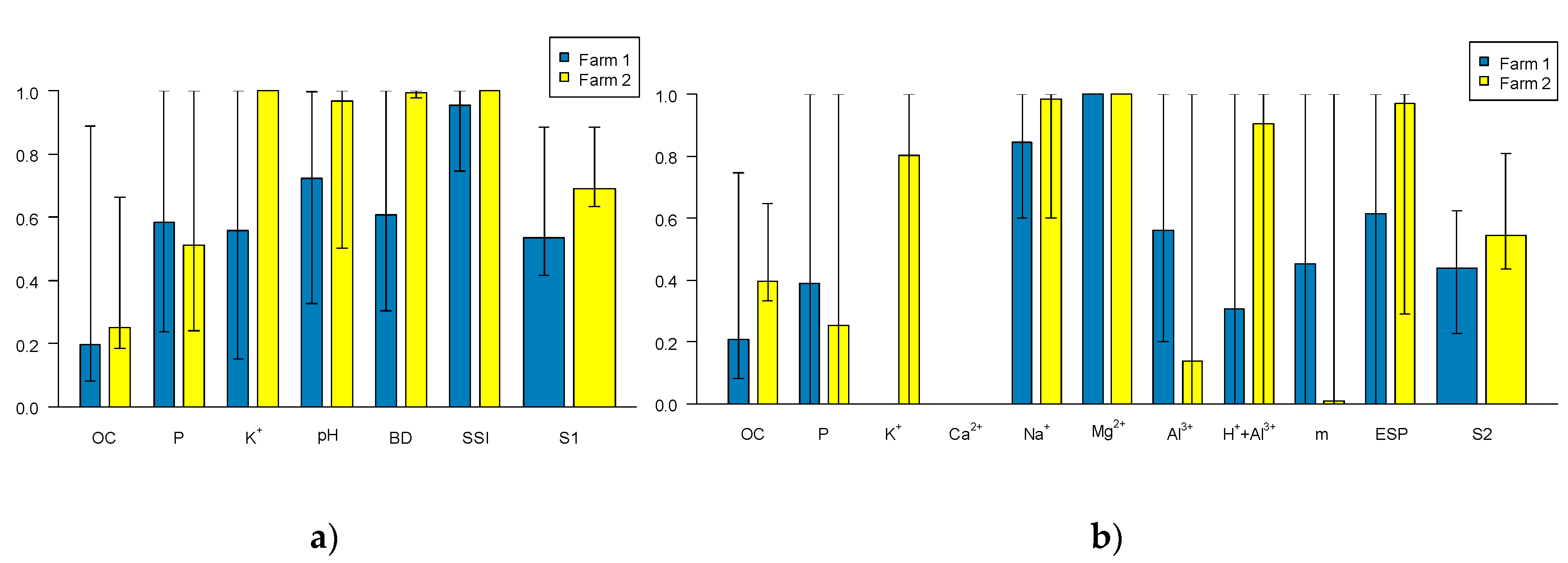
Table S7 shows the soil characteristics of all fields of both farms, which were used to calculate both soil indices. The area weighted means of S1 (Figure A5a, Table S8) show higher values for farm 2 for most of the indicators. An exception is P, where farm 1 has a slightly higher mean. The indicator OC has the most critical result, with a wide range of values for the single fields of each farm, but low mean scores. The average S1 for farm 2 is about 0.2 higher than for farm 1, but the highest scores are very similar for both farms.
The indicators of S2 show very diverse results across the fields of both farms (Figure A5b, Table S9). Some indicators score higher for farm 1, others for farm 2 or equal for both farms. The resulting S2 is about 0.1 higher for farm 2, indicating a slightly more preserved soil.
Comparing the results at field scale, it is noticeable that the area-weighted means of the final indices differ less between the methods than the single indicators. Both soil indices show low scores for OC, which is generally lost quickly in the Semiarid Northeast of Brazil after removing the native vegetation for agricultural use [7]. Farm 1 has on average a lower content of OC. This coincides with the fact that the land of farm 1 has been cultivated for decades, while farm 2 was cleared more recently. Additionally, soil texture of farm 1 is mainly sand, while at farm 2 loamy sand dominates (Table S7), which retains more water and nutrients. In contrast, P scores higher for farm 1, where the manure is processed in a manure compost system and additional manure is purchased. At farm 2, only the manure from the own cattle is used, without processing it in a manure compost.
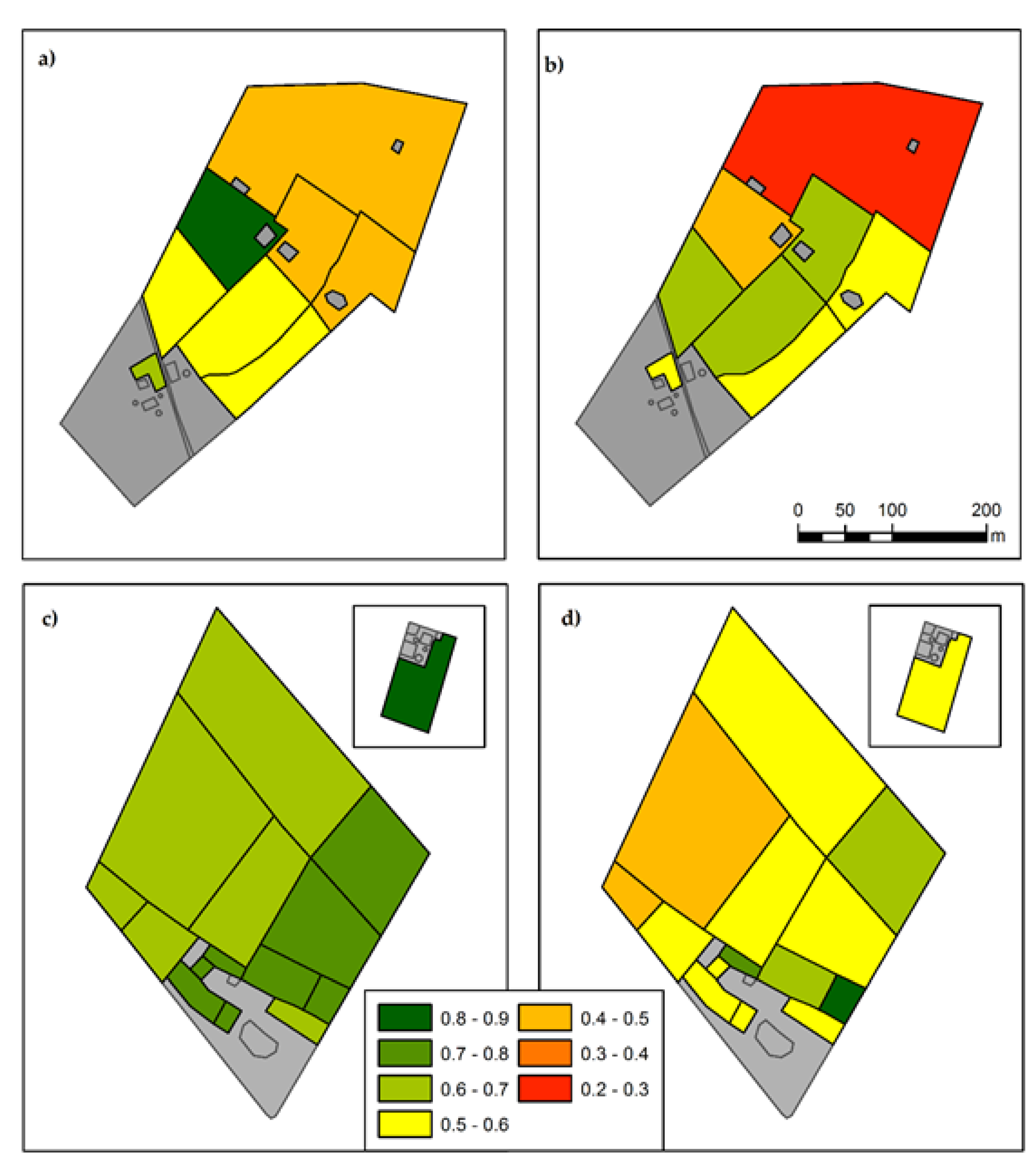
Looking at the soil indices of all fields to compare the differences between the farms and the methods (Figure A6) shows that, in general, both methods result in a better soil quality for farm 2, and S1 allocates to both farms a better soil quality than S2. Besides, S2 which uses more indicators and thresholds for indicator scoring elaborated particularly for Northeast Brazil, turns out to be more sensitive to show different patterns.

3.3. Cross-Scale Comparison

Comparing vulnerability across scales at index and indicator level (Figure 3) demonstrates that nested vulnerabilities can differ at each scale. At index level, M1 shows moderate vulnerability in both municipalities. M2 results in very low vulnerability for both municipalities for the corresponding time span (2002–2006). At farm scale, F1 shows very low vulnerability for both farms, while F2 evaluates farm 1 as slightly more vulnerable than farm 2. At field scale, both indices show moderate vulnerability for both farms, with a higher mean vulnerability for farm 1.
At different scales, different trends of vulnerability can be observed. At regional scale, M2 shows very low vulnerability for both municipalities in 2002–2006 (ly↑, rq↑) and very high vulnerability for Areial in 2012–2016 (ly↓, rq↓). At farm scale, F2 results for both farms in moderate vulnerability before 2000, which decreases to low vulnerability in 2014. Accordingly, in 2002–2006 vulnerability was decreasing at both scales, but in Areial this trend reversed in 2012–2016 at municipality scale. As F2 does not consider trends directly, an additional moment needs to be assessed in order to find out if at farm scale the trend changed as well.
At the indicator level, the seven indicators overlapping between municipality and farm scale have very different results (Figure 3). Irrigation is very rare in Areial and Remígio, resulting in very high vulnerability for both indicators at municipality and farm scale. Because of the dominantly crystalline subsoil, only very few farmers have access to wells. Accordingly, rainwater is the main water source, and it does not remain enough water for irrigation. Both investigated farms have no access to a well. Additionally, the equipment for highly efficient irrigation techniques is expensive.
Landownership shows low vulnerability at municipality and farm scale. The family of farm 1 inherited a part of the land and additionally bought land from neighbors. The family of farm 2 obtained the land after fighting for it together with the Landless Workers’ Movement and legalization by the land reform.
M1 results for Water in very low vulnerability in Areial and moderate vulnerability in Remígio, as in the latter more people are lacking access to water storage through wells, cisterns and artificial or natural lakes. The corresponding indicator of F1 is Access to water for livestock/consumption, resulting in very low vulnerability, while F2 evaluates Water autonomy with low vulnerability. Both farms have several cisterns, including a 52 000 l production cistern and small reservoirs at the pasture areas. Hence, both farms are independent in their water supply for consumption and livestock, even in years with reduced rainfall, but they need to use the water sparingly.
Production diversity due to M1 shows high and very high vulnerability for Areial and Remígio. In contrast, the farm scale indices result in much lower vulnerability. Both corresponding indicators of F1 (Crop diversification, Livestock diversification) result in very low vulnerability for both farms. F2 includes in Production diversity all types of agricultural production, resulting in low and very low vulnerability for farm 1 and 2, respectively.
At regional scale, the indicator Public policies is represented by M1 with the indicator Farms receiving technical assistance, resulting in very high vulnerability for Areial and low vulnerability for Remígio. At farm scale, many more forms of public policies are considered. F1 uses the indicators Access to state innovative support, to government emergency support and to remittances or state support, which lead to very low vulnerability for both farms. F2 shows for the indicator Access to public policies low vulnerability for farm 1 and very low vulnerability for farm 2. Since farm 2 is part of a settlement, founded due to the land reform, the family has had access to additional public policies, e.g., for the construction of the house and the communitarian seed bank.
Social participation is at regional scale represented by M1 with the indicator Farms whose heads are engaged in associations or unions. For Areial this results in very high vulnerability and for Remígio in high vulnerability. Differently, at farm scale both indices show very low or low vulnerability because both families are engaged in several organizations, e.g., Landless Workers’ Movement, unions of rural workers (Sindicatos dos Trabalhadores Rurais), community associations and cooperatives.
Income is represented by two indicators in M1: Dependence of farm income on animal and crop production and Municipal population engaged in agriculture. The first results in low vulnerability for Areial and moderate vulnerability for Remígio, while the second allocates moderate vulnerability to Areial and low vulnerability to Remígio. Both together evaluate the dependence of the municipality’s population on agricultural production, measuring the effects of yield- and livestock losses due to droughts, pests or diseases. M2, instead, results in high vulnerability for both municipalities. It considers the share of heads of households earning at least one minimum wage, independently if they work in the agricultural sector or not. At farm scale both indicators consider income diversity, resulting in very low (F1) and low (F2) vulnerability.
Comparing the indicators of Income used at regional and farm scale shows that a household can be classified as highly vulnerable with the concepts used at municipality scale because of a low income, exclusively from agriculture. On the same time, this household can result in low vulnerability due to the concept used at farm scale because of highly diversified agricultural activities, including drought tolerant income sources. The aspect of wealth and economic security is included in F1 explicitly, using additional indicators, such as Household wealth status, Ownership of means of transport, Savings and Access to credit. F2 complements the economic aspects more implicitly within the indicator Access to public policies.
Soil quality is the overlapping indicator between farm and field scale. In F1 it is represented by the indicator Extent of soil erosion, which is no outstanding problem on the considered farms, resulting in very low vulnerability. F2 considers with the indicator Soil fertility the natural soil fertility and management practices, such as a manure compost system or the cultivation of nitrogen-fixing legumes, resulting in low vulnerability for both farms. At field scale, the indicator OC of both soil indices shows a high average vulnerability with a wide range among the fields.

4. Discussion

4.1. Review of Indices for Vulnerability Assessment

Our systematic review provides a comprehensive overview of potential approaches to vulnerability assessment of smallholder farming systems. Including resilience and sustainability studies into our search proofed after all very appropriate. It required only little adaptation to transform resilience and sustainability indicators to comparable output ranges to existing vulnerability indices. It became evident that indices of the same scale showed at least an overlap of indicators. However, at field scale we could find only soil quality indices, consisting of a set of physical and chemical characteristics. Consequently, these indices go in more detail on soil quality but do not cover any of the other ecological, social or economic indicators used at municipality and farm scale.
As critical as the conceptual grounding appear (1) differences between static and dynamic indices, and (2) whether and how exposure is considered. These are critical points that highlight different perspectives on vulnerability. Static indices, such as M1, assess vulnerability at a certain point, allowing to compare between different municipalities. In contrast, M2 considers the development during time periods, evaluating if the vulnerability of a municipality is increasing or decreasing, using the municipality itself as reference. The differences in including or excluding exposure are also reflected in the conceptual progress of the IPCC, with Assessment Report 4 seeing vulnerability as a function of exposure amongst other factors [48], whereas more recently vulnerability is understood as a system´s quality independent from exposure [49]. In our study, the exposure is addressed only at regional scale: In M1, the average exposure is directly included with the aridity index, M2 indirectly includes the climatic impact within the indicator rq, which is expected to have a negative trend in drought years. But of course, exposure could be addressed also at lower scales.

4.2. Benefits of Intra- and Cross-Scale Comparison

An important benefit of using different methods and data at different scales is that the results complement each other. The intra-scale comparison at regional scale shows strong differences between the applied methods. As M1 and M2 show very different aspects of smallholder vulnerability, they were highly complementary and provided in sum a more complete picture. Together, they help to evaluate in which municipality the situation is deteriorating (M2) and which aspects contribute most to the municipality’s vulnerability (M1). Indicators used at just one scale can be taken as an approximation at other scales, especially when data availability does not allow the assessment at the other scale, such as climatic exposure, which is included only at regional scale.
Ideally, cross-scale vulnerability assessment would allow to explore systematically from larger to smaller scales of decision domains. In our case study on smallholder farmers in Northeast Brazil, it would give the farmers indication how to make their farms less vulnerable. For this, it would provide insight how they should distribute their resources (e.g., manure) best to increase soil fertility across their fields. And finally, it would provide insight how the farmers can organize themselves to reduce their vulnerability, for instance, through supporting networks.
In our case study, indicators used at different scales should therefore be more detailed at a smaller scale. In our assessment, the indicators Production diversity and Access to water include a lot more details on the farm level (F2) than on the municipality level (M1). While the indicator Production diversity in M1 is based only on the Agricultural Census, considering only manioc, corn, three varieties of beans, cow and goat milk and eggs, F2 takes into account all cultivated crops, such as fruits, vegetables, agave, fodder cactus, medicinal and ornamental plants. This way, kitchen gardens and other cultivations of small extent not registered in the Agricultural Census are included at farm scale [38]. Similarly, the indicator Access to water of M1 only describes the share of households with access to water in the form of cisterns, wells and lakes, but it does not consider if the households get enough water of the appropriate quality for their needs. F2 instead evaluates the water autonomy of the family in more detail, considering cisterns for drinking water and larger cisterns for small scale irrigation. Similar overlaps exist for soil fertility between F2 and both field-scale indices S1 and S2: F2 shows moderate vulnerability for the indicator soil fertility, which is consistent with the overall indices at field-scale, both providing deeper insights into the nutrient composition of the soil. However, both S1 and S2 do not include soil management indicators, although studies conducted in the Agreste and Cariri of Paraíba show that the use of green manure and manure compost systems are appropriate to maintain soil fertility and that agroforestry systems are useful to achieve a higher overall biomass production and stability towards climatic variations [50,51,52].

4.3. Limitations and Possible Improvements

Despite the clear value identified in the use of different indices at different scales, some issues arose in the application and in the interpretation of the results. First, as there are very few examples of cross-scale assessments available [29], a major challenge was to find an adequate set of indices. Second, a method for a systematic and effective comparison of the results was needed. The normalization, in particular, of the different indices and indicators was problematic especially in the case of M2, where the states II and IV both result in moderate vulnerability but actually they result from the opposite combination of positive and negative trends of ly and rq.
Limited data availability was the primary constraint for the number of farms included in the case study and the time slices addressed. Including more numerous and more diverse farms would have certainly improved the robustness of our results. But the time intense interviews as well as the soil analysis limited the analysis to only two farms. Furthermore, the delay of the Brazilian Agricultural Census of 2016 impeded a more recent calculation of M1 than 2006. Other information that had been gathered, could not be used appropriately as we limited ourselves to a comparison of already existing indices. For instance, land use and soil management information would have been available for each individual field, but the literature review only revealed field-scale indices that focused on soil composition. At regional scale, another data constraint originated from the characteristics of the municipalities. M2 uses input data of crop production and livestock numbers which do not differentiate between smallholders and other farmers and therefore its reliability is reduced when the share of smallholder farmland is below 50%. This was the case in more than half of the municipalities of the Borborema Territory, including Remígio.
All selected indices showed overlapping indicators between indices of the same scale and also with other scales. However, more overlapping indicators would have provided greater insights, in particular between scales. For our case study region, we suggest to include also soil data at the regional scale, which is available from Embrapa [35], and to consider the agricultural suitability of soil classes. Furthermore, we suggest to include local seed banks with natural seeds, which are gaining more and more importance for the farmers’ autonomy with the spreading of genetically modified and hybrid seeds. As the Agricultural Census does not inform about the origin of seeds, the share of organic farms could be used as an additional indicator to deduce the use of natural seeds at regional scale. At field scale, a more integrated index should also embrace management practices such as manure application, use of pesticides, crop rotation and land preparation, water availability from rain or irrigation and the varying demands of different crops.
The results at farm scale show how important it is that the methods are adapted to local conditions. F1 shows no differences between both farms, which could be explained by the similar degree of adaptation, but possibly also by the indicator thresholds. These were simply taken over from earlier studies [24,47], as the sample size in our case study was insufficient to adapt them to local conditions. In contrast, F2 shows clear differences between the two farms, as it was developed during the ASA/INSA research project for smallholder farming in the Semiarid Northeast of Brazil [26], and is highly sensitive to differences in the vulnerability of individual farms within the case study area.
Finally, for measuring changes in vulnerability, repeated assessments are needed. In the presented study, only M2 and F2 were assessed for two different moments or periods. The input data of both regional indices are publicly available for all Brazilian municipalities, facilitating a repeated assessment without new field campaigns. While M2 is mainly based on data which are published every year, M1 uses Census Data which are collected only once per decade. Both farm and field indices require individual data acquisition, for farm indices interviews and for field indices soil sampling and analyses in the laboratory. This makes the assessments more effortful than at regional scale. At field scale, selecting a reduced number of fields could reduce the effort per farm. Repeated assessments would also improve comparability across scales. Through the calculation of trends, different indices and indicators could be compared despite their thematic differences.

5. Conclusions

In the presented study we applied six indices to assess the vulnerability of two smallholder farms covering three different scales (region, farm, field). The indices have been selected based on data availability and their sensitivity to the specific agro-environmental conditions. Methodological limitations of the presented study were the constrained data availability, a small sample size at farm and field scale and the tight selection of indices at each scale.
Despite these methodological limitations, we identified a number of benefits in combining existing indices for a cross-scale vulnerability assessment. Intra-scale comparison at regional scale showed that the combination of an index of relative vulnerability with an index based on the trends of two indicators allows a better understanding than choosing one of them. At farm scale, one out of the two indices was well-adapted to local conditions and therefore produced more differentiated results. Intra-scale comparison was the most consistent at field scale because both soil indices were based on a concept of soil quality, producing outputs in the same value range.
The presented study highlights the benefits of cross-scale assessment and the potential to identify comprehensive sets of measures at different levels to reduce vulnerability of smallholder farmers. Practically, as data availability is the highest at regional scale, it is easiest to assess vulnerability first at this scale. The results are useful to define which aspects will be assessed at smaller scales. Then, the interviews at farm scale are helpful to include indicators, which are less detailed or not available in municipal statistics. Finally, soil sampling supports improved land management of the individual farm.
To optimize cross-scale vulnerability assessment, we propose to develop and apply a set of locally adapted indices (1) on nested scales (2) based on the same concept, (3) with more overlapping indicators und (4) with a similar spatial coverage of different scales. Ideally, the assessment should be repeated to investigate changes over time.
Our insights from the Northeast of Brazil can support further development of cross-scale vulnerability assessments for smallholder farming in many semi-arid environments worldwide. This is highly relevant, especially in the context of climate change.

Supplementary Materials

The following are available online at https://www.mdpi.com/2071-1050/12/9/3787/s1, Table S1: Reviewed indices for region, farm and field scale. Table S2: Results of municipality index 1. Table S3: Results of municipality index 2. Table S4: Results of farm index 1. Table S5: Results of farm index 2, farm 1. Table S6: Results of farm index 2, farm 2. Table S7: Analyzed and calculated soil characteristics. Table S8: Results of soil index 1. Table S9: Results of soil index 2.

Author Contributions

Conceptualization, S.D., A.W. and G.B.; Investigation, S.D.; Resources, A.M.P.-M.; Writing–original draft, S.D.; Writing–review & editing, A.M.P.-M., A.W. and G.B. All authors have read and agreed to the published version of the manuscript.

Funding

This research received no external funding.

Acknowledgments

We thank for the great support from the NGO AS-PTA (Agricultura Familiar e Agroecologia) (contact to the smallholder families, company to the field campaigns), INSA (National Institute of Semiaridity) (invitation for a research stay, use of the soil laboratory) and UFPB Areia (Federal University of Paraíba in Areia) (use of the soil laboratory). Besides, we acknowledge the support of the Deutsche Forschungsgemeinschaft and Open Access Publishing Fund of University of Potsdam.

Conflicts of Interest

The authors declare no conflict of interest.

Appendix A

Appendix A.1. Municipality Index 1

The indicators of M1 (Table A1) are normalized due to Equation (1). The subindices Sensitivity and Adaptive capacity are calculated from the average of the corresponding indicators. The indicator Farms without access to water storage considers natural and artificial lakes, wells and cisterns. For the indicator Product diversification, the Simpson Index of Diversity (SID) was calculated for the production of manioc, corn and three varieties of beans, cow and goat milk and eggs in kg, due to
SID = 1 i = 1 k P i 2 ,
with Pi: share of production in kg of the ith product (crop or animal product). Typically, the SID is calculated with the share of area used for each crop [53]. In this study, it was opted to use produced kg to allow the combination of crop and animal products in one index.
Exposure is based on only one indicator, which is the inverse of the Aridity Index due to [54]:
AI = P ETP ,
with AI: Aridity Index; P: precipitation; ETP: potential evapotranspiration, both average annual (mm). The Aridity Index was calculated using ArcGIS Desktop 10.3. The gridded values of average annual potential evapotranspiration from Xavier, King and Scanlon [39] with a resolution of 0.25° × 0.25° and the annual precipitation isohyets [33] were interpolated (tools spline and topo to raster, respectively). Then, the mean Aridity Index was derived for each municipality (tool zonal statistics) and inverted by subtraction from 1.
Finally, M1 was calculated due to the equation
M 1 = E + S + ( 1 AC ) 3 ,
with S: Sensitivity; E: Exposure; AC: Adaptive capacity. The output index ranges from 0 to 1, indicating very low to very high vulnerability for each municipality, relative to the study context.
Table A1. Subindices and indicators, municipality index 1 (based on [21,46]).
Sub-IndicesIndicators *
Sensitivity (S)Dependence of farm income on crop and animal production (%)
Municipal population engaged in agriculture (%)
Farms without access to water storage (%)
Farms with rainfed farming (%)
Adaptive capacity (AC)Product diversification
Farms in which the producer is the landowner (%)
Farms whose heads can read and write (%)
Farms whose heads are engaged in associations or unions (%)
Farms receiving technical assistance (%)
Farms with access to electric energy supply (%)
Exposure (E)Aridity Index (AI)
* All indicators refer to smallholder farms/agriculture.

Appendix A.2. Municipality Index 2

The input data of M2 are from IBGE [38]: harvested area, yield and livestock number are from the yearly Municipal Agricultural and Livestock Production Census. Grassland area is used from the Brazilian Agricultural Census 2006 and income distribution (% with minimum wage) from the Demographic Census 2010, as they are not available for more recent years or a finer time resolution.
The yearly values of yield-oriented labor (ly) and resource quality (rq) are calculated using the equations
ly y , i = j = 1 4 lyd j A y , ij ( c ) + j = 5 6 lyd j N y , ij   and
rq y , i = j = 1 71 m y , ij f ij j = 1 71 A y , ij
with j: 6 classes of agricultural activities; lydj: relative specific labor demand (Table A2); A(c)y,ij and Ny,ij: harvested area and livestock quantity of class j in municipality i and year y; Ay,ij (j = 1–70): harvest areas of the 70 crops for municipality i in year y; Ay,ij (j = 71): respective pasture area for livestock; my,ij (j = 1–70): yields (tons) of the 70 crops for municipality i in year y; my,ij (j = 71): livestock in livestock units for municipality i in year y (cow, ox, buffalo: 1 unit; pig, horse, donkey: 0.5; goat, sheep: 0.1). The factor
f ij = m ¯ ij A ¯ ij
is calculated from the annual means of the years 2002–2006 and 2012–2016, respectively, to normalize crop yields and livestock numbers and allow a relative comparison of crops and livestock.
Table A2. Relative specific labor demand of agricultural activities (based on [20], more livestock classes added).
ActivityRelative-Specific Labour Demand (lyd) *Examples
Cereal crops1Beans, corn, rice
Roots, tubers7Manioc, cashew nuts, cotton
Specialized crops20Tomatoes, melons, mangoes
Pastures0.3
Cattle, buffalos2
Pigs, horses, donkeys1
Goats, sheep0.25
* In the first three classes labor demand relates to the harvested area.
With a linear regression, the five-year trends of ly and rq are calculated to allocate the states I–IV. The probability of a shift from state II to state III increases with the share of smallholders earning more than the Existential budget. Therefore, the share of households where the head of household earns at least one minimum wage (510 R$) is considered. The linear regression to estimate the trends of ly and rq is evaluated with the coefficient of determination (R²). Both trends should have an R² of at least 0.9 for a statistically significant allocation to one of the four qualitative states.

Appendix A.3. Farm Index 1

Table A3 shows the indicators of F1 applied in this study, adapted from Bishop and Fuller [24] and Oxfam [47].
Table A3. Subindices, weighting and indicators of farm index 1, based on Bishop and Fuller [24] and Oxfam [47].
SubindicesIndicators
Livelihood viability (30%)Land ownership, household wealth status,
Livelihood diversification, household food security
Crop diversification, production
Livestock diversification, herd size
Ownership of means of transport
Livestock lost to drought or diseases, vaccination
Drought preparedness practice
Access to markets
Innovation potential (20%)Attitudes towards new livelihood practices
Adoption of improved production techniques
Access to credit, state innovative support
Ability to influence others
Access to contingency resources and support (20%)Group participation
Access to government emergency support
Savings, grain storage
Access to remittances or state support
Ownership of fungible livestock
Integrity of the natural and built environment (15%)Extent of soil erosion
Access to irrigation, water for livestock/consumption
Access to grazing land
Tree planting
Social and institutional capability (15%)Access to drought warning information
Drought preparedness plan
Institutions supporting adaptation
Solidarity in the community
Thresholds and weighting of each indicator, see Table S4.

Appendix A.4. Farm Index 2

Table A4 shows the evaluated subindices and indicators of F2.
Table A4. Subindices and indicators of farm index 2, based on Petersen et al. [26].
SubindicesIndicators
AutonomySeed autonomy
Water autonomy
Feed autonomy
Food security
Soil Fertility
ResponsivityProduction diversity
Market diversity
Income diversity
Gender equityGender equity
Social integrationSocial participation
Access to public policies

Appendix A.5. Soil Index 1

As the indicator Visual evaluation of soil structure was not available, it was substituted by the physical indicators bulk density (BD) and structural stability index (SSI). The scoring of indicators where more is better uses Equation (8) and where less is better Equation (9):
S = 1 1 + ( B UT x UT ) 2.5   and  
S = 1 1 + ( B LT x LT ) 2.5   ,
with S: indicator score; x: measured indicator value; B: baseline value, UT: upper threshold; and LT: lower threshold. For indicators with a mid-point optimum, both equations are used. The soil indicators with the parameters for the scoring curve are specified in Table A5. For measured values equal or beyond the threshold, the equation is not defined, consequently the score is set to 0 or 1, depending if the value is above or below the threshold. Finally, S1 is calculated by weighted additive aggregation due to the equation
S 1 = i = 1 n W i S i
with Si: indicator score; n: number of indicators integrated in the index; Wi: weighted value of the indicator. The indicator output ranges from 0 to 1, indicating very low to very high soil quality.
Table A5. Soil Indicators with weighting and scoring curve parameters, soil index 1, based on Cherubin et al. [27].
IndicatorUnitWeightingLTBUTOPScoring Curve
OCg/kg0.331017.525 More is better
Pmg/dm30.112816 More is better
K+mmolc/dm30.110.40.81.6 More is better
pH-0.114.55/88.56Optimum
BDg/cm30.171.51.651.8 Less is better
SSI%0.17579 More is better
Soil characteristics BD: bulk density; K+: potassium; OC: soil organic carbon; P: phosphorus; pH: potential of hydrogen in solution of H2O 1:2.5; SSI: structural stability index. Scoring curve parameters B: baseline value; LT: lower threshold; OP: optimum point; UT: upper threshold.

Appendix A.6. Soil Index 2

Table A6 shows the thresholds and scoring indication of the indicators of S2.
Table A6. Soil indicators with thresholds and scoring indication, soil index 2 (based on Vendruscolo and Perez-Marin 2017, unpublished).
IndicatorUnitPreservedDegradedScoring *
OCg/kg28.063.13Pres = max
Pmg/kg10.886.15Pres = max
K+mg/kg150.14112.25Pres = max
Ca2+cmolc/kg7.094.84Pres = max
Na+cmolc/kg0.060.16Deg = max
Mg2+cmolc/kg2.142.83Deg = max
Al3+cmolc/kg0.020.12Deg = max
H++Al3+cmolc/kg3.021.84Pres = max
m%0.361.91Deg = max
ESP%0.561.81Deg = max
Soil characteristics Al3+: aluminum(III); Ca2+: calcium; ESP: exchangeable sodium percentage; H++Al3+: potential acidity; K+: potassium; m: saturation of exchangeable Al3+; Mg2+: magnesium; Na+: sodium; OC: soil organic carbon; P: phosphorus. * Indicates if the maximum value was found at preserved or degraded areas.

Appendix B

Figure A1. (a) Results of municipality index 1 (M1) [21,46] with subindices AC: Adaptive capacity; E: exposure; S: Sensitivity; (b) Results of municipality index 2 (M2) [20].
Sustainability 12 03787 g0a1
Figure A2. Annual precipitation of 5 rain gauges in the study area from 2000–2016 and average annual rainfall of Alagoa Nova (data source: AESA [34]).
Sustainability 12 03787 g0a2
Figure A3. Intra-scale comparison of municipality indices; (a) M1: municipality index 1 for 2006 and (b) M2: municipality index 2 for 2002–2006, with indication of the share of family farmland.
Sustainability 12 03787 g0a3
Figure A4. (a) Results of farm index 1 (note that results are not distinguished between farms because the values are the same), (b) farm index 2 before 2000 and (c) farm index 2 in 2004, always sub-indices and index values.
Sustainability 12 03787 g0a4
Figure A5. Results of (a) soil index 1 (S1) and (b) soil index 2 (S2); Area-weighted means and range of occurring values of soil indicators Al3+: aluminum (III); Ca2+: calcium; ESP: exchangeable sodium percentage; H++Al3+: potential acidity; K+: potassium; m: saturation of exchangeable Al3+; Mg2+: magnesium; Na+: sodium; OC: soil organic carbon; P: phosphorus; pH: potential of hydrogen in solution of H2O 1:2.5; SSI: structural stability index.
Sustainability 12 03787 g0a5
Figure A6. Intra-scale comparison of soil indices; (a) Soil index 1 (S1), farm 1, (b) soil index 2 (S2), Figure 1. (c) S1, farm 2, (d) S2, farm 2; soil indices range: 0–1 (very low–very high soil quality).
Sustainability 12 03787 g0a6

References

  1. Fischer, G.; Shah, M.; Velthuizen, H. Van Climate Change and Agricultural Vulnerability. In Proceedings of the A Special Report, World Summit on Sustainable Development, Johannesburg, South Africa, 26 August–4 September 2002. [Google Scholar]
  2. Morton, J.F. The impact of climate change on smallholder and subsistence agriculture. Proc. Natl. Acad. Sci. USA 2007, 104, 19680–19685. [Google Scholar] [CrossRef] [Green Version]
  3. Lowder, S.K.; Skoet, J.; Raney, T. The Number, Size, and Distribution of Farms, Smallholder Farms, and Family Farms Worldwide. World Dev. 2016, 87, 16–29. [Google Scholar] [CrossRef] [Green Version]
  4. Machado, H.F.; Bennati, P.; Guilles, M.; Rocha, P.; Lima, A.; Vasconcelos, I. Climate change and impacts on family farming in the North and Northeast of Brazil; International Policy Centre for Inclusive Growth Working Paper 141; International Policy Centre for Inclusive Growth: Brasilia, Brazil, 2016. [Google Scholar]
  5. Lima, R.; da, C.C.; Cavalcante, A.; de, M.B.; Pérez-Marin, A.M. Desertificação e Mudanças Climáticas no Semiárido Brasileiro; INSA-PB: Campina Grande, Brazil, 2011; ISBN 9788564265028. [Google Scholar]
  6. IBGE Censo Agropecuário 2017. Resultados Preliminares; Instituto Brasileiro de Geografia e Estatística: Rio de Janeiro, Brazil, 2018. [Google Scholar]
  7. Menezes, R.S.C.; Garrido, M.S.; Perez Marin, A.M. Fertilidade dos solos no semi-árido. In XXX Congr. Bras. Ciência do Solo; Rio de janeiro: Embrapa Solos, Brazil, 2005; p. 30. [Google Scholar]
  8. Downing, T.E.; Patwardhan, A. Assessing Vulnerability for Climate Adaptation. In Adaptation Policy Frameworks for Climate Change: Developing Strategies, Policies and Measures; Cambridge University Press: Cambridge, GB, USA, 2005; pp. 69–87. [Google Scholar]
  9. Pandey, R.; Meena, D.; Aretano, R.; Satpathy, S.; Semeraro, T.; Kumar Gupta, A.; Rawat, S.; Zurlini, G. Socio-ecological Vulnerability of Smallholders due to Climate Change in Mountains: Agroforestry as an Adaptation Measure. Chang. Adapt. Socio-Ecol. Syst. 2015, 2, 26–41. [Google Scholar]
  10. Luers, A.L.; Lobell, D.B.; Sklar, L.S.; Addams, C.L.; Matson, P.A. A method for quantifying vulnerability, applied to the agricultural system of the Yaqui Valley, Mexico. Glob. Environ. Chang. 2003, 13, 255–267. [Google Scholar]
  11. Fellmann, T. The Assessment of Climate Change-Related Vulnerability in the Agricultural Sector: Reviewing Conceptual Frameworks; Pablo de Olavide University: Seville, Spain, 2012; ISBN 9780123985293. [Google Scholar]
  12. Tao, S.; Xu, Y.; Liu, K.; Pan, J.; Gou, S. Research Progress in Agricultural Vulnerability to Climate Change. Adv. Clim. Chang. Res. 2011, 2, 203–210. [Google Scholar] [CrossRef]
  13. Descheemaeker, K.; Oosting, S.J.; Homann-Kee Tui, S.; Masikati, P.; Falconnier, G.N.; Giller, K.E. Climate change adaptation and mitigation in smallholder crop–livestock systems in sub-Saharan Africa: A call for integrated impact assessments. Reg. Environ. Chang. 2016, 16, 2331–2343. [Google Scholar] [CrossRef] [Green Version]
  14. Füssel, H.-M. Review and Quantitative Analysis of Indices of Climate Change Exposure, Adaptive Capacity, Sensitivity, and Impacts; World Bank: Washington, DC, USA, 2009. [Google Scholar]
  15. Böhringer, C.; Jochem, P. Measuring the Immeasurable: A Survey of Sustainability Indices. Ecol. Econ. 2007, 63, 1–8. [Google Scholar]
  16. Füssel, H.M. How inequitable is the global distribution of responsibility, capability, and vulnerability to climate change: A comprehensive indicator-based assessment. Glob. Environ. Chang. 2010, 20, 597–611. [Google Scholar]
  17. Lesnikowski, A.; Ford, J.; Biesbroek, R.; Berrang-Ford, L.; Heymann, S.J. National-level progress on adaptation. Nat. Clim. Chang. 2016, 6, 261–264. [Google Scholar] [CrossRef]
  18. Awolala, D.O.; Ajibefun, I.A. Rice Farmers’ Vulnerability to Extreme Climate: Deploying Local Adaptation Finance in Ekiti State, Nigeria. World Environ. 2015, 5, 91–100. [Google Scholar]
  19. Eakin, H.; Winkels, A.; Sendzimir, J. Nested vulnerability: Exploring cross-scale linkages and vulnerability teleconnections in Mexican and Vietnamese coffee systems. Environ. Sci. Policy 2009, 12, 398–412. [Google Scholar] [CrossRef]
  20. Sietz, D.; Untied, B.; Walkenhorst, O.; Lüdeke, M.K.B.; Mertins, G.; Petschel-Held, G.; Schellnhuber, H.J. Smallholder agriculture in Northeast Brazil: Assessing heterogeneous human-environmental dynamics. Reg. Environ. Chang. 2006, 6, 132–146. [Google Scholar] [CrossRef]
  21. Lindoso, D.P.; Rocha, J.D.; Debortoli, N.; Parente, I.C.I.; Eiró, F.; Bursztyn, M.; Rodrigues-Filho, S. Climate Change and Vulnerability to drought in the semiarid: The case of smallholder farmers in the brazilian northeast. In Climate Change in Brazil: Economic, Social and Regulatory Aspects; da Motta, R.S., Hargrave, J., Luedemann, G., Gutierrez, M.B.S., Eds.; World Bank: Washington, DC, USA, 2011; ISBN 9788578111281. [Google Scholar]
  22. IPCC Managing the Risks of Extreme Events and Disasters to Advance Climate Change Adaptation. In Special Report of the Intergovernmental Panel on Climate Change; Field, C.B.; Barros, V.; Stocker, T.F.; Dahe, Q.; Dokken, D.J.; Ebi, K.L.; Mastrandrea, M.D.; Mach, K.J.; Plattner, G.-K.; Allen, S.K.; et al. (Eds.) IPCC: Cambridge, UK, 2012. [Google Scholar]
  23. Blesh, J.; Wittman, H. “Brasilience”: Assessing Resilience in Land Reform Settlements in the Brazilian Cerrado. Hum. Ecol. 2015, 43, 531–546. [Google Scholar] [CrossRef]
  24. Bishop, D.; Fuller, R. Resilience in Nicaragua: Impact Evaluation of Climate Change Adaptation among Small Scale Producers; Effectiveness Review Series 2014/15; Oxfam GB: Oxford, UK, 2015. [Google Scholar]
  25. Fernandes, L.A.D.O.; Woodhouse, P.J. Family farm sustainability in southern Brazil: An application of agri-environmental indicators. Ecol. Econ. 2008, 66, 243–257. [Google Scholar] [CrossRef]
  26. Petersen, P.; da Silveira, L.M.; Fernandes, G.B.; Almeida, S.G. de Método de análise econômico-ecológica de Agroecossistemas, 1st ed.; Articulação Nacional de Agroecologia/AS-PTA: Rio de Janeiro, Brazil, 2017; ISBN 9788587116284. [Google Scholar]
  27. Cherubin, M.R.; Karlen, D.L.; Cerri, C.E.P.; Franco, A.L.C.; Tormena, C.A.; Davies, C.A.; Cerri, C.C. Soil quality indexing strategies for evaluating sugarcane expansion in Brazil. PLoS ONE 2016, 11, e0150860. [Google Scholar] [CrossRef]
  28. Perez Marin, A.M.; Rogé, P.; Altieri, M.A.; Ulloa Forero, L.F.; Silveira, L.; Oliveira, V.M.; Domingues-Leiva, B.E. Agroecological and social transformations for coexistence with semi-aridity in Brazil. Sustainability 2017, 9, 990. [Google Scholar] [CrossRef] [Green Version]
  29. Scholes, R.J.; Reyers, B.; Biggs, R.; Spierenburg, M.J.; Duriappah, A. Multi-scale and cross-scale assessments of social-ecological systems and their ecosystem services. Curr. Opin. Environ. Sustain. 2013, 5, 16–25. [Google Scholar] [CrossRef]
  30. Reidsma, P.; Ewert, F.; Oude Lansink, A.; Leemans, R. Vulnerability and adaptation of European farmers: A multi-level analysis of yield and income responses to climate variability. Reg. Environ. Chang. 2009, 9, 25–40. [Google Scholar] [CrossRef] [Green Version]
  31. Sietz, D. Regionalisation of global insights into dryland vulnerability: Better reflecting smallholders’ vulnerability in Northeast Brazil. Glob. Environ. Chang. 2014, 25, 173–185. [Google Scholar] [CrossRef] [Green Version]
  32. da Silveira, L.M.; Freire, A.G.; Diniz, P.C.O. Polo da Borborema: Ator contemporâneo das lutas camponesas pelo território. Rev. Agric. 2010, 7, 13–19. [Google Scholar]
  33. AESA Geo Portal. Available online: http://geoserver.aesa.pb.gov.br/geoprocessamento/geoportal/ shapes.html (accessed on 1 October 2017).
  34. AESA Meteorologia–Chuvas. Available online: http://www.aesa.pb.gov.br/aesa-website/meteorologia-chuvas (accessed on 15 January 2017).
  35. Embrapa Solos UEP Recife. Available online: www.uep.cnps.embrapa.br/solos/index.html (accessed on 12 December 2017).
  36. Embrapa Sistema Brasileiro de Classificação de Solos, 2nd ed.; Sistema Brasileiro de Classificação de Solos: Brasília, Brazil, 2013; ISBN 85-85864-19-2.
  37. FAO. International Soil Classification System for Naming Soils and Creating Legends for Soil Maps; World Soil; FAO: Rome, Italy, 2015; ISBN 9251055114. [Google Scholar]
  38. IBGE Sistema IBGE de Recuperação Automática-SIDRA. Available online: sidra.ibge.gov.br (accessed on 20 December 2017).
  39. Xavier, A.C.; King, C.W.; Scanlon, B.R. Daily gridded meteorological variables in Brazil (1980–2013). Int. J. Climatol. 2015, 2659, 2644–2659. [Google Scholar] [CrossRef] [Green Version]
  40. Campos, D.V.B.; de Calderano, S.B.; Teixeira, W.G.; Viana, J.H.M. (Eds.) Embrapa Manual de Métodos de Análise de Solo, 2nd ed.; Embrapa Solos: Rio de Janeiro, Brazil, 2011; ISSN 1517-2627. [Google Scholar]
  41. Reynolds, W.D.; Drury, C.F.; Tan, C.S.; Fox, C.A.; Yang, X.M. Use of indicators and pore volume-function characteristics to quantify soil physical quality. Geoderma 2009, 152, 252–263. [Google Scholar] [CrossRef]
  42. do Carmo, D.L.; Silva, C.A. Métodos de Quantificação de Carbono e Matéria Orgânica em Resíduos Orgânicos. Rev. Bras. Ciência do Solo 2012, 36, 1211–1220. [Google Scholar] [CrossRef]
  43. Turner, B.L. Vulnerability and resilience: Coalescing or paralleling approaches for sustainability science? Glob. Environ. Chang. 2010, 20, 570–576. [Google Scholar] [CrossRef]
  44. Douxchamps, S.; Debevec, L.; Giordano, M.; Barron, J. Monitoring and evaluation of climate resilience for agricultural development–A review of currently available tools. World Dev. Perspect. 2017, 5, 10–23. [Google Scholar] [CrossRef]
  45. Miller, F.; Osbahr, H.; Boyd, E.; Thomalla, F.; Bharwani, S.; Zervogel, G.; Walker, B.; Birkmann, J.; van der Leeuw, S.; Rockstrom, J.; et al. Resilience and vulnerability: Complimentary or conflicting concepts? Ecol. Soc. 2010, 15, 1–25. [Google Scholar] [CrossRef]
  46. Lindoso, D.P.; Rocha, J.D.; Debortoli, N.; Parente, I.I.; Eiró, F.; Bursztyn, M.; Rodrigues-Filho, S. Integrated assessment of smallholder farming’s vulnerability to drought in the Brazilian Semi-arid: A case study in Ceará. Clim. Chang. 2014, 127, 93–105. [Google Scholar] [CrossRef]
  47. Oxfam, G.B. Disaster Risk Reduction Programming in Ethiopia’s Somali Region. In Project Effectiveness Review; Full Technical Report; Oxfam GB: Oxford, UK, 2013. [Google Scholar]
  48. Pachauri, R.K.; Reisinger, A. (Eds.) IPCC Climate Change 2007: Contribution of Working Groups I, II and III to the Fourth Assessment Report of the Intergovernmental Panel on Climate Change; Cambridge University Press: Cambridge, UK; New York, NY, USA, 2007. [Google Scholar]
  49. IPCC Climate Change 2014: Impacts, Adaptation and Vulnerability. Part A: Global and Sectoral Aspects. In Contribution of Working Group II to the Fifth Assessment Report of the Intergovernmental Panel on Climate Change; Field, C.B.; Barros, V.R.; Dokken, D.J.; Mach, K.J.; Mastrandrea, M.D.; Bilir, T.E.; Chatterjee, M.; Ebi, K.L.; Estrada, Y.O.; Genova, R.C.; et al. (Eds.) Cambridge University Press: Cambridge, UK; New York, NY, USA, 2014. [Google Scholar]
  50. Menezes, R.S.C.; Silva, T.O. da Mudanças na fertilidade de um Neossolo Regolítico após seis anos de adubação orgânica. Rev. Bras. Eng. Agrícola Ambient. 2008, 12, 251–257. [Google Scholar] [CrossRef] [Green Version]
  51. da Silva, E.D.; Perez Marin, A.M.; Vendruscolo, J. Efeito de adubos orgânicos no crescimento de Zea mays L. em um Neossolo Regolítico. Cad. Agroecol. 2015, 10, 1–5. [Google Scholar]
  52. Martins, J.C.R.; Menezes, R.S.C.; Sampaio, E.V.S.B.; dos Santos, A.F.; Nagai, M.A. Produtividade de biomassa em sistemas agroflorestais e tradicionais no Cariri Paraibano. Rev. Bras. Eng. Agric. Ambient. 2013, 17, 581–587. [Google Scholar] [CrossRef] [Green Version]
  53. Mofya-Mukuka, R.; Hichaambwa, M. Factors Influencing Smallholder Crop Diversification in Zambia and the Implications for Policy; Indaba Agricultural Policy Research Institute Working Paper 112; Indaba Agricultural Policy Research Institute: Lusaka, Zambia, 2016. [Google Scholar]
  54. UNESCO. UNESCO Map of the World Distribution of arid Regions; UNESCO: Paris, France, 1979; ISBN 9788578110796. [Google Scholar]
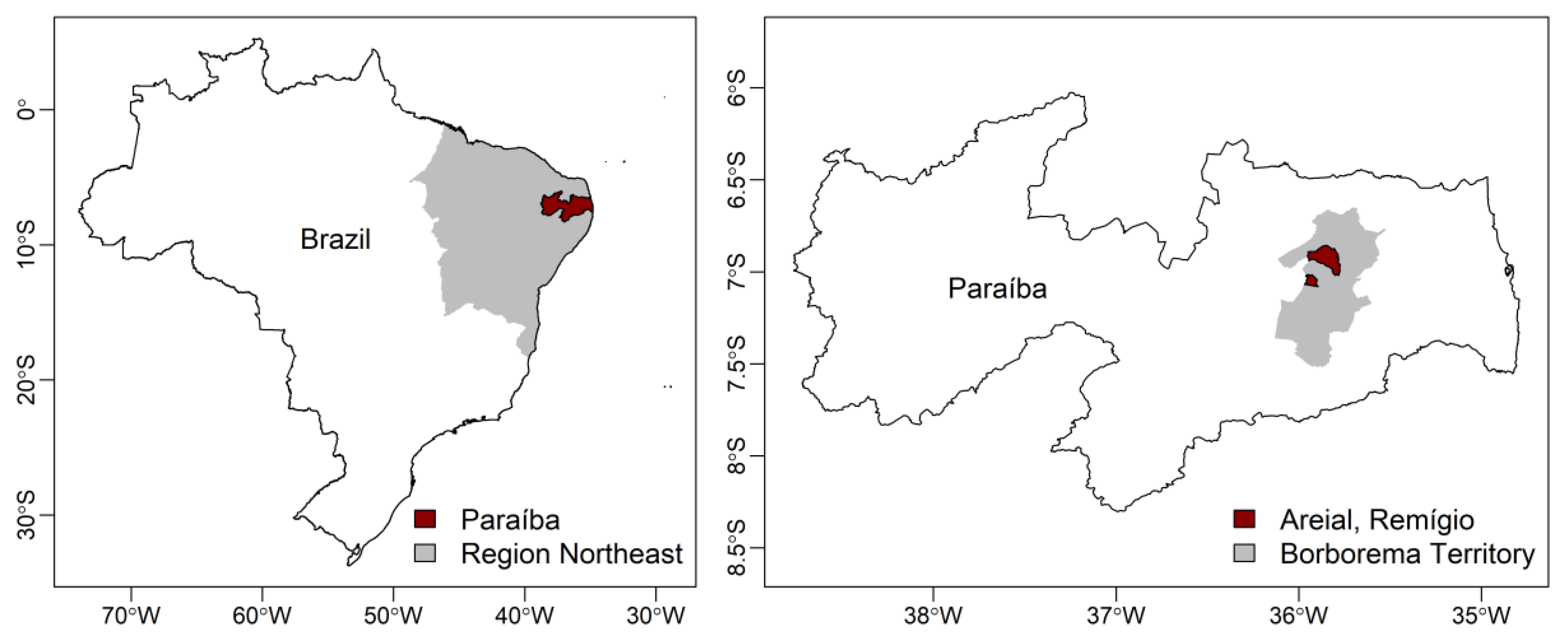
Figure 1. Location of the Study Area in the State of Paraíba, Northeast Brazil.
Sustainability 12 03787 g001
Figure 2. Overlapping indicators of the applied indices, intra-scale and across scales.
Sustainability 12 03787 g002
Figure 3. Cross-scale comparison of indices (left) and overlapping indicators (right), from left to right: irrigation, landownership, soil quality, water, production diversity, public policies, social participation, income; all indices and indicators normalized to 0–1 (very low–very high vulnerability), the indicators of F2 are shown only for 2014 as there is no cross-scale comparison possible for the first time step (before 2000).
Sustainability 12 03787 g003