Parametric Assessment of Trend Test Power in a Changing Environment

Abstract

In the context of climate and environmental change assessment, the use of probabilistic models in which the parameters of a given distribution may vary in accordance with time has reinforced the need for appropriate procedures to recognize the “statistical significance” of trends in data series arising from stochastic processes. This paper introduces a parametric methodology, which exploits a measure based on the Akaike Information Criterion (AIC_Δ), and a Rescaled version of the Generalized Extreme Value distribution, in which a linear deterministic trend in the position parameter is accounted for. A Monte Carlo experiment was set up with the generation of nonstationary synthetic series characterized by different sample lengths and covering a wide range of the shape and scale parameters. The performances of statistical tests based on the parametric AIC_Δ and the non-parametric Mann-Kendall measures were evaluated and compared with reference to observed ranges of annual maxima of precipitation, peak flow, and wind speed. Results allow for sensitivity analysis of the test power and show a strong dependence on the trend coefficient and the L-Coefficient of Variation of the parent distribution from the upper-bounded to the heavy-tailed special cases. An analysis of the sample variability of the position parameter is also presented, based on the same generation sets.

1. Introduction

The environment and climate change are recognized worldwide as an interdisciplinary area of investigation which reaches into different fields of research (e.g., [1,2]). It regards earth sciences such as climatology, atmospheric physics and chemistry, and hydrology. It is also an area of investigation in life sciences, including ecology and the biology of any living organism on earth, and has strong implications for social, economic, and industrial sciences, considering new branches of emerging risks and cascading effects. Due to such interactions, multi-disciplinary approaches should also be more developed, as proposed by Metzger et al. [3] and Cagle et al. [4], considering that, even in contiguous fields of environmental analyses and applications, the perspective and scale of investigations can be very different, ranging from global to regional, catchment-size and at-site assessment of physical quantities and their observations [5,6].

This paper deals with trend assessment in extreme events of environmental variables and how it affects their frequency distribution. We focus on annual maxima of peak flow, rainfall, and wind speed, which trigger natural hazards such as floods, storms, sea waves, and storm surges. The same approach could also be adapted to describe other phenomena, such as heatwaves and droughts.

Our perspective is typical of the hydrological sciences and is strongly based on the analysis of time series of variables modeled as stochastic processes. Moreover, this is the approach adopted in the civil engineering practice, which is focused on providing sustainable solutions for living and developing human activity and security in terms of adaptation to environmental changes and societal preparedness for natural hazards.

Over the last few decades, increasing attention has been dedicated by scientists to statistical analyses of environmental random variables. Interest in this field is reasonably motivated by the need for finding reliable approaches aimed at detecting and understanding the nature of climate change. This has led to a vast amount of study into the detection of trends, change points, or shifts in time series, collecting a wide range of tests, each one with proper peculiarities and characteristics (e.g., [7]). A paramount example is the well-known Mann–Kendall (MK) test, which is probably the most used tool in environmental analysis for investigating the statistical significance of an observed trend and belongs to the vast category of Null-Hypothesis Statistical Tests (NHST). It should be remarked that while many studies are produced by exploiting NHST, a significant number of other papers warn of theoretical and practical drawbacks to their use (e.g., [8,9]). Some of these warnings deal with the misuse of statistical tests. Two types of error may occur during the application of these tests: the first one (called Type I error) is to reject the null hypothesis when it is true, the second one (Type II error) is to accept the null hypothesis when it is false. In practice, the probability of committing a Type I error can be estimated theoretically or numerically, thanks also to the increasing availability of tools (such as R software) able to provide results in a few steps. It should be noted that the ease of applying these approaches and of managing results has often led to misuse or misconceptions of their outputs. In this regard, while much attention has always been paid to the Type I error, much less care has been dedicated to evaluating the Type II error, which should be considered more important [10,11,12].

In this debate, the American Statistical Association (ASA) dedicated a journal special issue “Moving to a World Beyond ‘p < 0.05’”, to encourage researchers to be “more thoughtful when applying statistical significance tests” [13].

The need for giving an appropriate evaluation of the power of the MK test was highlighted, among others, by Totaro et al. [14]. They followed the approach proposed by Yue et al. [15] that produced a numerical evaluation of the MK test power for Generalized Extreme Value (GEV) distributed samples. Wang et al. [16] provided a practical relationship for a proper power assessment of specific time series.

In environmental applications in particular, the length of the observed series required to reach an acceptable power value could be very different according to the variable’s parent distribution and the strength of the trend [10,14,15,16]. It could be much shorter for temperature and humidity time series than for runoff and precipitation time series that usually show higher space–time variability.

Focusing attention on the hydrological field, a proper approach to the theory of stochastic processes is a conditio sine qua non for addressing the analysis correctly. In particular, the occurrence and magnitude of the hydrological variables can be considered as an outcome of a process that can be characterized by one or more probability distributions. As a consequence, a correct analysis should rely on a process of identification able to discern between stationary and nonstationary models [17,18]. From this point of view, the goal of this kind of analysis is shifted to the model selection framework in which nonstationarity is identified as a deterministic time-dependence in parameters of the parent distribution [19].

According to Yohe et al. [20], a sustainable approach to risk, hazard, and disaster risk management entails both disaster risk reduction and adaptation to climate change. One way to pursue these targets is by changing guidelines and procedures of design to account for the increasing magnitude of events due to climate change. The evaluation of frequency distributions for design purposes is typically treated with a parametric approach, through probabilistic models with parameters estimated from observed data (see [21]). Therefore, the parent distribution is exploited to find quantiles of the assigned probability of exceedance. The parametric procedure proposed here allows for the detection of trends to be used for design purposes accounting for nonstationary conditions. On the other hand, non-parametric approaches are very commonly adopted in the environmental analysis because they only exploit observed data and do not require the identification of a parent distribution and its parameters. A typical example is the MK test.

Following this path of investigation, Totaro et al. [14] showed that both parametric and non-parametric tests for trend assessment suffer from the following issues: (i) the results of the test are dependent on the parent distribution and (ii) for weak trends, i.e., for small values of the trend coefficient, the test power reduces to low and unacceptable values.

They carried out a sensitivity analysis on a set of parameters of the GEV distribution that was representative of the annual maximum rainfall series. For a series of length L = 30, depending on the parent parameter values, trend coefficients up to 0.8 mm per year may lead to power values below the conventional threshold of 0.8. The situation improves for longer series nevertheless, and the problem persists also for L = 50; the power is still too low for trend values up to 0.5 mm/y for a Gumbel distributed parent and up to even larger values for heavy-tailed distributions.

They conclude that, as already acknowledged in many other scientific fields such as medical and social sciences [22,23], the evaluation of power should be always performed to assess the real physical meaning of the test outcomes and, to such purpose, they proposed the use of a parametric approach, which allows for a simple power evaluation by numerical Monte Carlo experiments, applicable to any specific context.

The goals of this paper are (i) to further develop the use of parametric tests, based on model selection criteria (Akaike Information Criterion, AIC_Δ) described in Section 2, (ii) to provide a generalized methodology which exploits a Rescaled GEV distributed variable, and (iii) to extend the evaluations performed by Totaro et al. [14] to parameter ranges covering the variability of different physical variables suitable for climate change assessment. Such a development is of great practical interest because, in principle, it provides a general tool for estimating the power value and assesses the real statistical significance on extreme values of any variable of environmental interest.

To this purpose, we investigated the range of variability of three different annual maximum series, including precipitation, peak flow, and wind speed. In particular, the search was conducted focusing on world datasets found in literature following the GEV distribution and exploiting parameter values as a function of L-moments ratios [24], widely employed in regional frequency analysis.

The paper is structured as follows: in Section 2, the MK and AIC_Δ tests are illustrated and a Rescaled GEV distribution is derived; in Section 3, the explored world datasets and the range-values of L-moments ratios are described. Section 4 focuses on the power of the above-mentioned tests as a function of L-Coefficient of Variation (L-CV) and trend slope. Considerations about the sampling variability of the parent distribution position parameters are also reported. Section 5 summarizes the main conclusions of this work and focuses on the main implications of these findings in research perspectives.

2. Methodologies

In this paragraph, three main topics are described. In Section 2.1, the parametric AIC_Δ test is proposed. In Section 2.2, the Rescaled GEV distribution is defined, specifying relationships between dimensionless parameters and theoretical GEV L-moments. Finally, in Section 2.3, the sensitivity analysis and the procedure followed for the evaluation of test power are illustrated.

2.1. The Akaike Information Criteria Based Test

NHST are precious tools for identifying and quantifying particular properties of recorded data. Their correct use includes a conscious interpretation of their outputs for supporting deductions in the framework of climate change.

The non-parametric Mann–Kendall test [25,26] is widely diffused in environmental analysis, due to its simplicity in the evaluation of the statistical significance of a trend. Its structure and main properties are reported in Appendix A.

In this paper, we introduce a new parametric test based on the use of the Akaike Information Criterion (AIC; [27]) for model selection (e.g., [28,29,30]). AIC is probably the most used likelihood-based criterion for model selection. It is legitimate to consider its success due to simplicity and conceptual basis. It is based on the Kullback–Leibler distance measure. From a practical approach, defined as ${\mathbf{\theta }}_{st}$ and ${\mathbf{\theta }}_{ns}$ the set of parameters characterizing the probabilistic models, and with $\widehat{\ell }\left(·\right)$ the maximized value of the log-likelihood function, AIC is defined as

$$AIC=-2\widehat{\ell }\left(\mathbf{\theta }\right)+2k$$

(1)

where k is the number of parameters of the selected model. According to this criterion, the model with the lowest value of AIC should be the better one among the set of models examined.

Following the idea of exploiting model selection criteria for detecting changes in time series analysis, Totaro et al. [14] proposed the use of $AI{C}_R$, defined as the ratio between the AIC values obtained, respectively, from nonstationary and stationary candidate models. They showed that, through Monte Carlo numerical experiments, is possible to evaluate $AI{C}_R$ statistical distribution and find the $AI{C}_{R,\alpha }$ threshold value corresponding to an assigned level of significance $\alpha$. In this way, ${AIC}_{\mathrm{R},\mathsf{\alpha }}$ $AI{C}_R$ can be used as a test variable whose power depends on the parent distribution shape and scale parameters.

In this paper, the same procedure is applied to AIC_Δ [31], defined as the difference:

$$AI{C}_{\Delta }=AI{C}_{ns}-AI{C}_{st}$$

(2)

which assumes positive values if the stationary model is the preferred one and negative values in the opposite case.

The AIC_Δ distribution can be numerically computed with the aim to find a threshold value AIC_Δ,α for an α level of significance, by the following procedure:

• Generate a certain number of samples (e.g., 10,000) from an assigned stationary model, assumed as the null hypothesis of the test;
• Compute AIC_Δ for all samples and determine its empirical probability distribution;
• Evaluate the threshold value AIC_Δ,α corresponding to an assigned level of significance $\alpha$ (here set to 0.05), that will be used for accepting or rejecting the null hypothesis of stationarity of point 1.

2.2. Rescaled GEV Distribution

The Generalized Extreme Value (GEV) distribution was introduced in the hydrological literature by Jenkinson [32]. Its success in practical applications is mainly due to its ability for contemplating Gumbel (EV1), Fréchet (EV2), and Weibull (EV3) distributions as special cases. Assuming z is an annual maximum stationary process variable, with parameter set $\mathbf{\theta }$, the GEV cumulative distribution function is expressed as

$$F\left(z,\mathbf{\theta }\right)=\{\begin{array}{c}exp\left\{-{\left[1+\epsilon \left(\frac{z-\zeta }{\sigma }\right)\right]}^{-\raisebox{1ex}{$1$}\!\left/ \!\raisebox{-1ex}{$\epsilon $}\right.}\right\} \epsilon \ne 0\\ exp\left\{-exp\left[-\left(\frac{z-\zeta }{\sigma }\right)\right]\right\} \epsilon =0\end{array}$$

(3)

where $\zeta$,$\sigma$, and $\epsilon$ are, respectively, position, scale, and shape parameters. Analytical positions require that $\sigma$ must be strictly positive. Several methods are available for estimating GEV parameters in the stationary case, such as Maximum Likelihood, probability-weighted moments, or L-moments. This latter approach, introduced by Hosking [24], makes use of linear combinations of order statistics. For the aim of this paper, it is useful to report theoretical expressions of the following L-moment values (first and second-order) and ratios (L-CV, L-Skewness, L-Kurtosis) [33]:

	$\epsilon <1$	$\epsilon =0$
First-order (Mean)	${\lambda }_1=\zeta -\frac{\sigma }{\epsilon }\left[1-\mathsf{\Gamma }\left(1-\epsilon \right)\right]$	${\lambda }_1=\zeta +\sigma \gamma$	(4)
Second-order	${\lambda }_2=\frac{\sigma \left(1-2^{\epsilon }\right)\mathsf{\Gamma }\left(1-\epsilon \right)}{\epsilon }$	${\lambda }_2=\sigma \ln 2$	(5)
L-CV	$\tau =\frac{\sigma \left(1-2^{\epsilon }\right)\mathsf{\Gamma }\left(1-\epsilon \right)}{\sigma \left[1-\mathsf{\Gamma }\left(1-\epsilon \right)\right]-\epsilon \zeta }$	$\tau =\frac{\sigma \ln 2}{\sigma \gamma +\zeta }$	(6)
L-Skewness	${\tau }_3=\frac{2\left(1-3^{\epsilon }\right)}{\left(1-2^{\epsilon }\right)}-3$	${\tau }_3=\frac{\ln \left(9/8\right)}{\ln 2}$	(7)
L-Kurtosis	${\tau }_4=\frac{\left[5\left(1-4^{\epsilon }\right)-10\left(1-3^{\epsilon }\right)+6\left(1-2^{\epsilon }\right)\right]}{\left(1-2^{\epsilon }\right)}$	${\tau }_4=\frac{\left(16\ln 2-10\ln 3\right)}{\ln 2}$	(8)

where $\gamma$ is the Euler’s constant.

Equation (3) can be extended to the case of nonstationarity, simply assuming that its three parameters can be modeled as a function of time [19,34]:

$${\mathbf{\theta }}_{\mathit{n}\mathit{s}}=\left[\zeta ,\sigma ,\epsilon \right]\to {\mathbf{\theta }}_{\mathit{n}\mathit{s}}=\left[{\zeta }_t,{\sigma }_t,{\epsilon }_t\right].$$

(9)

Whilst from a theoretical perspective, the ${\mathbf{\theta }}_{\mathit{n}\mathit{s}}$ parameter set in Equation (9) could be modeled in a variety of ways; in this paper, we adopt the simplest time-dependent behavior by considering $\sigma$ and $\epsilon$ constant values and only the position parameter to follow a linear trend dependence, as

$${\zeta }_t={\zeta }_0+{\zeta }_1·t$$

(10)

This requires only four parameters to be estimated [ ${\zeta }_0,{\zeta }_1,\sigma ,\epsilon$]. This can be done via the Maximum Likelihood method. Several R packages can be used for this purpose, among which are extRemes [35] and ismev.

It is also possible to adopt a general GEV expression, with $\mathbf{\theta }=$[ ${\zeta }_0,{\zeta }_1,\sigma ,\epsilon$], by introducing Equation (10) in Equation (3) assuming

$$\zeta ={\zeta }_t$$

(11)

After this substitution in Equation (3), the GEV is nonstationary if ${\zeta }_1^{}\ne 0,$ and stationary if ${\zeta }_1^{}=0$ with $\zeta ={\zeta }_0^{}$.

The range of values of the four parameters is strongly linked to observed time series, leading to a variety of values and cases depending on the hydrological variable taken into account (e.g., rainfall, flow peak, wind speed). In order to produce results of general interest, in this paper a dimensionless formulation in Equations (3)–(11) is proposed by introducing the rescaled aleatory variable $z^{\prime }$ defined as

$$z^{\prime }=\frac{z}{{\zeta }_0}.$$

(12)

Following this transformation also the position and scale parameters are rescaled by ${\zeta }_0$, while the shape parameter (which is dimensionless by definition) remains unchanged, hence we obtain

$${{\zeta }^{\prime }}_t=\frac{{\zeta }_t}{{\zeta }_0}, {{\zeta }^{\prime }}_0=\frac{{\zeta }_0}{{\zeta }_0}=1, {{\zeta }^{\prime }}_1=\frac{{\zeta }_1}{{\zeta }_0}, {\sigma }^{\prime }=\frac{\sigma }{{\zeta }_0} \mathrm{and} {\epsilon }^{\prime }=\epsilon$$

(13)

to provide the Rescaled GEV written as

$$F\left(z^{\prime },{\mathbf{\theta }}^{\prime }\right) =\{\begin{array}{c}exp\left\{-{\left[1+\epsilon \left(\frac{z^{\prime }-{{\zeta }^{\prime }}_{1}t-1}{{\sigma }^{\prime }}\right)\right]}^{-\raisebox{1ex}{$1$}\!\left/ \!\raisebox{-1ex}{$\epsilon $}\right.}\right\} \epsilon \ne 0\\ \\ exp\left\{-exp\left[-\left(\frac{z^{\prime }-{{\zeta }^{\prime }}_{1}t-1}{{\sigma }^{\prime }}\right)\right]\right\} \epsilon =0\\ \end{array}$$

(14)

with ${\mathbf{\theta }}^{\prime }=\left[{{\zeta }^{\prime }}_1,{\sigma }^{\prime },\epsilon \right]$, which is nonstationary if ${\zeta }_1^{\prime }\ne 0,$ and stationary if ${\zeta }_1^{\prime }=0$.

The first and second-order L-moments are also rescaled to give

	$\epsilon <1$	$\epsilon =0$
First-order (Mean)	${{\lambda }^{\prime }}_1=\frac{{\lambda }_1}{{\zeta }_0}={{\zeta }^{\prime }}_t-\frac{{\sigma }^{\prime }}{\epsilon }\left[1-\mathsf{\Gamma }\left(1-\epsilon \right)\right]$	${{\lambda }^{\prime }}_1=\frac{{\lambda }_1}{{\zeta }_0}={{\zeta }^{\prime }}_t+{\sigma }^{\prime }\gamma$	(15)
Second-order	${{\lambda }^{\prime }}_2=\frac{{\lambda }_2}{{\zeta }_0}=\frac{{\sigma }^{\prime }\left(1-2^{\epsilon }\right)\mathsf{\Gamma }\left(1-\epsilon \right)}{\epsilon }$	${{\lambda }^{\prime }}_2=\frac{{\lambda }_2}{{\zeta }_0}={\sigma }^{\prime }\ln 2$	(16)

After rescaling, the L-CV

$${\tau }^{\prime }=\frac{{{\lambda }^{\prime }}_2}{{{\lambda }^{\prime }}_1}=\tau$$

(17)

and the other L-moment ratios (L-Skewness and L-Kurtosis) remain unaffected. It is worth noting that both the mean and the L-CV values change in time according to Equations (15)–(17). In the following we will refer to the stationary (or initial) L-CV value evaluated as

	$\epsilon <1$	$\epsilon =0$
L-CV	${\tau }^{\prime }=\tau =\frac{{\sigma }^{\prime }\left(1-2^{\epsilon }\right)\mathsf{\Gamma }\left(1-\epsilon \right)}{{\sigma }^{\prime }\left[1-\mathsf{\Gamma }\left(1-\epsilon \right)\right]-\epsilon }$	${\tau }^{\prime }=\tau =\frac{{\sigma }^{\prime }\ln 2}{{\sigma }^{\prime }\gamma +1}$	(18)

With these statements, a generalization of results provided by Totaro et al. [14] can be provided.

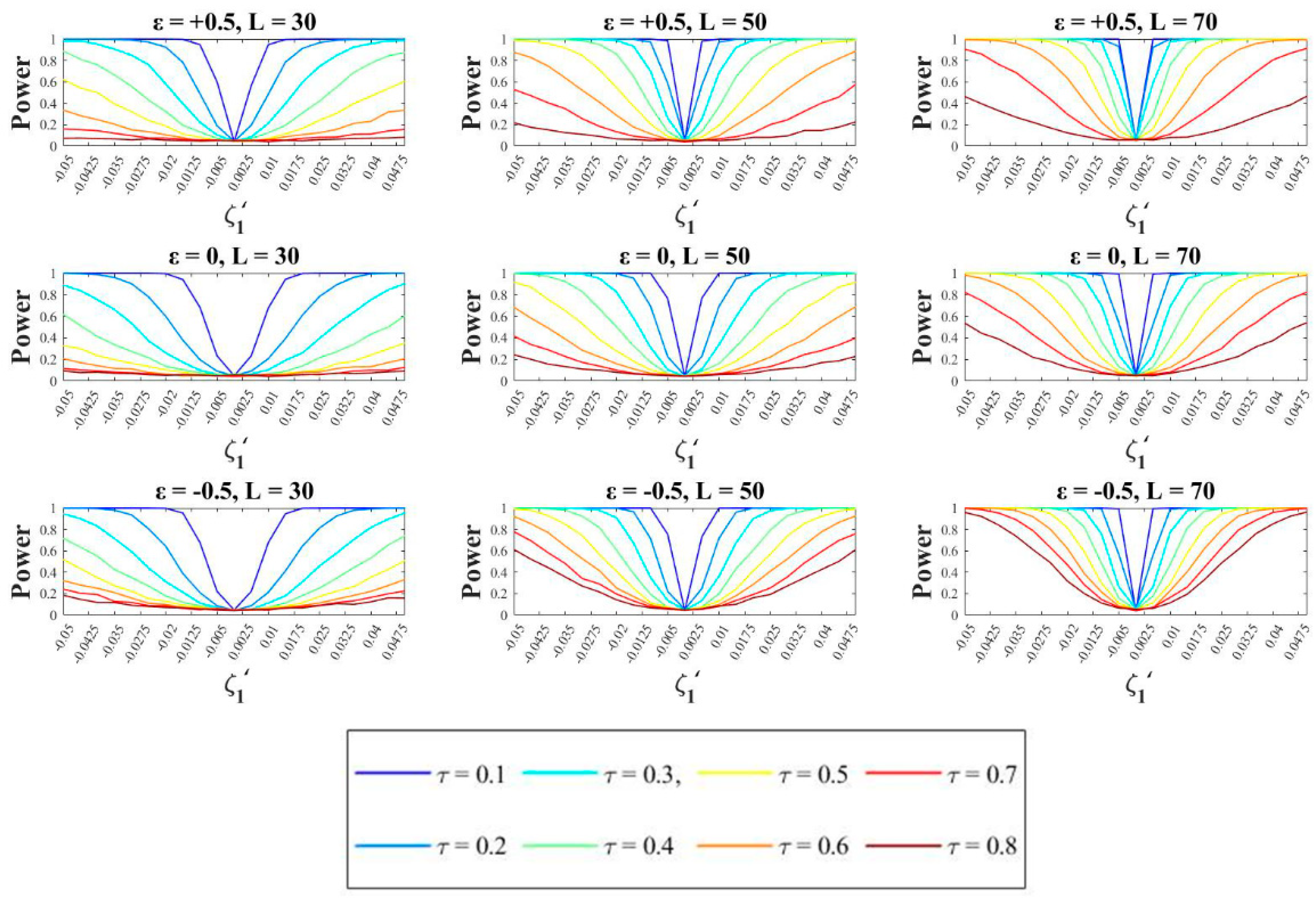
2.3. Power Evaluation and Sensitivity Analysis

The application of NHST is based on the definition of two important quantities: level of significance and power. The first one is defined as the probability of committing a Type I error, i.e., to incorrectly reject the null hypothesis when it is true. Defining the level of significance is a required task and its use is widespread, also sometimes in comparison with observed p-values. On the other hand, it has to be remarked that equal or even more importance should be given to the probability of a Type II error, i.e., the incorrect acceptance of the null hypothesis when it is false. Complementary to this one is the power of the test, defined as the probability to correctly reject the null hypothesis when it is false. Compared to the huge number of studies dealing with the statistical hypothesis testing of stationarity in environmental sciences, only a few papers focus on the evaluation of power and its crucial role (e.g., [9,10]). Among these, Totaro et al. [14] highlighted the need to establish a conventional power value as a minimum for accepting test results and also suggested the use of a parametric approach to evaluate the test power accounting for the length of data series and parent parameter values. Thus, applying both the MK and AIC_Δ and assuming as a null hypothesis that data are originated from a stationary model, the test power can be evaluated simulating a certain number of samples N from a nonstationary model and counting the number of series $N_r$ in which the null hypothesis is rejected:

$$power=\frac{N_r}{N}$$

(19)

The sensitivity analysis presented in this paper was carried out repeating such a procedure for sets of N = 2000 series generated by a Rescaled GEV parent distribution, parameter sets obtained by the combination of different values of ${{\zeta }^{\prime }}_1$, σ’, $\epsilon$, and different sample lengths L.

3. Literature Parameter Range of Extreme Rainfall, Flow Peak, and Wind Speed

Datasets of three hydrological variables (annual maxima of rainfall, flood, and wind) were analyzed for performing this analysis. The following sub-paragraphs report the main sample properties of each of these variables. In

Table 1. Database features and observed parameter ranges of annual maximum rainfall.

Location	Sites	L-CV	L-Skewness	L-Kurtosis	Length	Reference
Iran (southwestern)	154	0.130–0.600	−0.180–0.750	0.050–0.700	10–52	[41]
World	15,137	N.A.	−0.160–0.760	−0.060–0.730	40–163	[40]
Saudi Arabia (Medina Region)	20	0.294–0.442	0.118–0.376	0.033–0.338	28–50	[42]
Turkey (Cekerek watershed)	17	0.133–0.205	−0.083–0.468	−0.029–0.453	11–76	[43]
Pakistan (east-northeast)	23	0.168–0.429	0.095–0.487	0.043–0.381	24–60	[44]
Malaysia (West Coast)	30	0.142–0.267	0.046–0.447	0.096–0.382	33–38	[45]
Italy (Sicily)	124	0.240	0.244	0.168	>20	[46]

,

Table 2. Database features and observed parameter ranges of annual maximum flow peak.

Location(s)	Sites	L-CV	L-Skewness	L-Kurtosis	Length	Reference
India (Kerala)	43	0.125–0.530	−0.013–0.581	0.003–0.400	13–47	[51]
Pakistan (Punjab)	7	0.351–0.453	0.242–0.457	0.063–0.355	36–85	[52]
Iran (Karkheh watershed)	42	0.272–0.501	0.001–0.575	−0.048–0.381	13–43	[53]
Italia (Sicily)	55	0.202–0.871	−0.169–0.854	−0.010–0.818	10–64	[54]
New Zealand (South Canterbury and West Coast)	20	0.081–0.560	−0.171–0.640	−0.065–0.511	11–52	[55]
Italy, Austria, Slovakia	1132	0.015–0.769	−0.121–0.773	−0.158–0.713	9–182	[56]
Turkey	543	0.100–0.600	−0.050–0.600	0.000–0.400	15–57	[57]
Australia	61	0.160–0.646	−0.192–0.586	−0.058–0.536	21–72	[58]

and

Table 3. Database features and observed parameter ranges of annual maximum wind speed.

Location	Sites	L-CV	L-Skew	L-Kurtosis	Length	Reference
Pakistan	9	0.061–0.145	−0.250–0.283	0.080–0.326	7–25	[68]
Iran	19	0.100–0.320	0.030–0.700	0.080–0.660	17–53	[69]
United States	6	0.0958–0.1821	0.0406–0.5107	0.0838–0.3150	19–35	[33]
Canada	235	0.030–0.160	−0.220–0.350	−0.040–0.400	>17	[64]

, the main database features listed hereafter by the column title are reported:

Location: nation(s) of investigated sites, with the indication of a particular area of interest (if present)

Sites: number of sites considered

L-CV: the observed range of $\tau$; if only the mean value is reported, this number is shown (the same for ${\tau }_3$ and ${\tau }_4$)

L-Skewness: the observed range of ${\tau }_3$

L-Kurtosis: the observed range of ${\tau }_4$

Length: the range of the observed series length (L)

Reference

If values are deduced from a visual inspection of a plot, they are reported in italic.

3.1. Literature Studies on Extreme Rainfall

The use of L-moments for regional frequency analysis is widely diffused in hydrological practice. Several applications of this approach can be found about the analysis of annual maximum daily rainfall [36,37,38,39].

Table 1 reports studies illustrating ranges of the main L-moments ratios. In particular, Koutsoyiannis and Papalexiou [40] collected a world dataset of annual maximum daily rainfall, providing reliable information about the state of the art of the distribution of their statistical characteristics.

It is worth noting that the L-CV has a relatively limited range of variation, which is between 0.13 and 0.44. The L-Skewness, instead, moves from negative (about −0.13) to positive values up to 0.5. An exception is represented by the Iran case study, where the upper limits are 0.6 (L-CV) and 0.75 (L-Skewness).

3.2. Literature Studies on Extreme Flow Peak

Flood frequency analysis is a diffused technique for evaluating the design values of peak flow. Its importance is mainly due to the strong impact that floods exercise on societies and assets. A wide literature is available on methods and approaches for the implementation of statistical analysis, especially in regional contexts. In this framework, numerous studies were realized (e.g., [47,48,49,50]). In Table 2, an overview of L-moments ratios from the analyzed datasets is provided.

3.3. Literature Studies on Extreme Wind Speed

Jung and Schindler [59] provided a wide and complete review of the selection of wind speed distributions. Several studies have assessed the best-fitting distributions and methodologies for wind speed prediction [60,61]. Fawad et al. [62] highlighted the importance of extreme wind speed distribution in different fields, such as renewable energies, structural designs, and meteorology. The use of L-moments for extreme value analysis was applied by [63,64,65,66]. Hundecha et al. [67] exploited the application of the nonstationary GEV model for investigating the annual maxima of wind speed in Canada.

In Table 3, summary statistics for annual maximum wind speeds are reported.

4. Results and Discussion

The sensitivity analysis was carried out evaluating the test power as described in Section 2.3 and repeating such a procedure for sets of N = 2000 series generated by a Rescaled GEV parent distribution with three different values of $\epsilon$ accounting for different GEV shapes: upper-bounded EV3 ($\epsilon =-0.5$), EV1 ($\epsilon =0$), and heavy-tailed EV2 ($\epsilon =0.5$). Furthermore, according to the database analysis reported in Section 3.1, Section 3.2, and Section 3.3, we selected a range of L-CV which goes from 0.1 to 0.8 and sampled such a range with a step of 0.1. Then, we exploited the relationship (18) to evaluate the σ’ values, according to the chosen set of $\epsilon$ and L-CV values. Resulting σ’ values are reported in

Table 4. Values of σ’ used in the Monte Carlo simulations for different combinations of ε and L-Coefficient of Variation (L-CV).

${\mathit{\sigma }}^{\prime }$		L-CV
		0.1	0.2	0.3	0.4	0.5	0.6	0.7	0.8
ε	−0.5	0.201	0.422	0.655	0.934	1.233	1.568	1.945	2.373
	0	0.157	0.341	0.577	0.865	1.236	1.730	2.421	3.457
	+0.5	0.076	0.172	0.298	0.470	0.718	1.108	1.809	3.442

.

We considered different values of the trend ${\zeta }_1^{\prime }$ ranging from −0.05 to 0.05 (± 5% per year) with a step of 0.005, and three sample lengths L (30,50,70). Considering all combinations of $\epsilon$, ${\sigma }^{\prime }$, ${\zeta }_1^{\prime }$, and L, we obtained 1512 different generation sets

4.1. Power of AIC_Δ and MK Tests for Different Values of ε and L-CV.

For each of the underlying distributions described above, Figure 1 and Figure 2 show the dependence between the rescaled trend coefficient ${\zeta }_1^{\prime }$ and the power of the AIC_Δ and MK tests, according to three defined values of the shape parameter $\epsilon$ $\left(-0.5,0,0.5\right)$, sample size L $\left(30, 50, 70\right)$, and L-CV $\left(0.1:0.1:0.8\right)$. All curves obtained with values of the trend ${\zeta }_1^{\prime }\ne 0$ are generated by a nonstationary parent distribution.

In general, AIC_Δ shows a higher power than MK, except for upper-bounded GEV, where MK is slightly better performing. Such differences are more evident for heavy-tailed GEV and smaller sample length. Nevertheless, both show strong dependence from ${\zeta }_1^{\prime }$, ε, L-CV, and L. The power, for all ε values, decreases with increasing L-CV and decreasing $\left|{\zeta }_1^{\prime }\right|$ and L.

It is interesting to remark that, apart from the well-known dependence from trend value, sample size, and shape parameter, a strong influence is exerted by the L-CV values. As an example, the left column of Figure 1 shows results for the minimum considered sample length (L = 30)—for all the ε values and the entire range of trend values considered, the AIC_Δ power is below 0.8 when L-CV is higher than 0.5. For further increase of L-CV, it collapses to values as small as 0.2. This situation gradually expires when increasing the sample size up to 70. Faster growth in power performances is detected for the upper-bounded GEV (ε = −0.5).

A similar but even worse situation is found for the MK test. For $L=30$ and all the values of $\epsilon$, the test is characterized by power values lower than 0.8 if L-CV is higher than 0.3. Such an implication is remarkable because it affects the reliability of this test for all series characterized by high variability. As for AIC_Δ, there is an obvious improvement in the performances as the sample size increases. These results are in perfect agreement with the findings of Yue et al. [15], who analyzed the MK test power from generation performed with GEV parent distribution, with different values of the trend, coefficient of variation, and sample size. They are also consistent with the results shown by Wang et al. [16] and extend the range of climatic variability explored by Totaro et al. [14].

Results shown above suggest that for different combinations of ε, L-CV, and L it is possible to evaluate the range of trend values ${\zeta }_1^{\prime }$ providing acceptable power values. For some cases, we had to extend the range of ${\zeta }_1^{\prime }$ beyond ±5% per year, up to values that allow the reaching of an acceptable power value.

This analysis is reported with reference to absolute values of the trend because the power curves are all symmetric with respect to the vertical axis ${\zeta }_1^{\prime }=0.$ In Figure 3 is reported the dependence from L-CV of the minimum absolute value of the trend coefficient ${\zeta }_1^{\prime }$, which is necessary for achieving the conventional power value of 0.8. This dependence is shown for different $\epsilon$ and L values, both for AIC_Δ and MK tests.

The role of L-CV is crucial for a proper interpretation of results in this case too. Small L-CV values correspond to smaller $\left|{\zeta }_1^{\prime }\right|$ ranges, with an increase of up to 300% when L-CV varies from 0.1 to 0.8. In principle, looking at Figure 3, it is possible to evaluate whether the chosen test is applicable for a series of known distribution and given length.

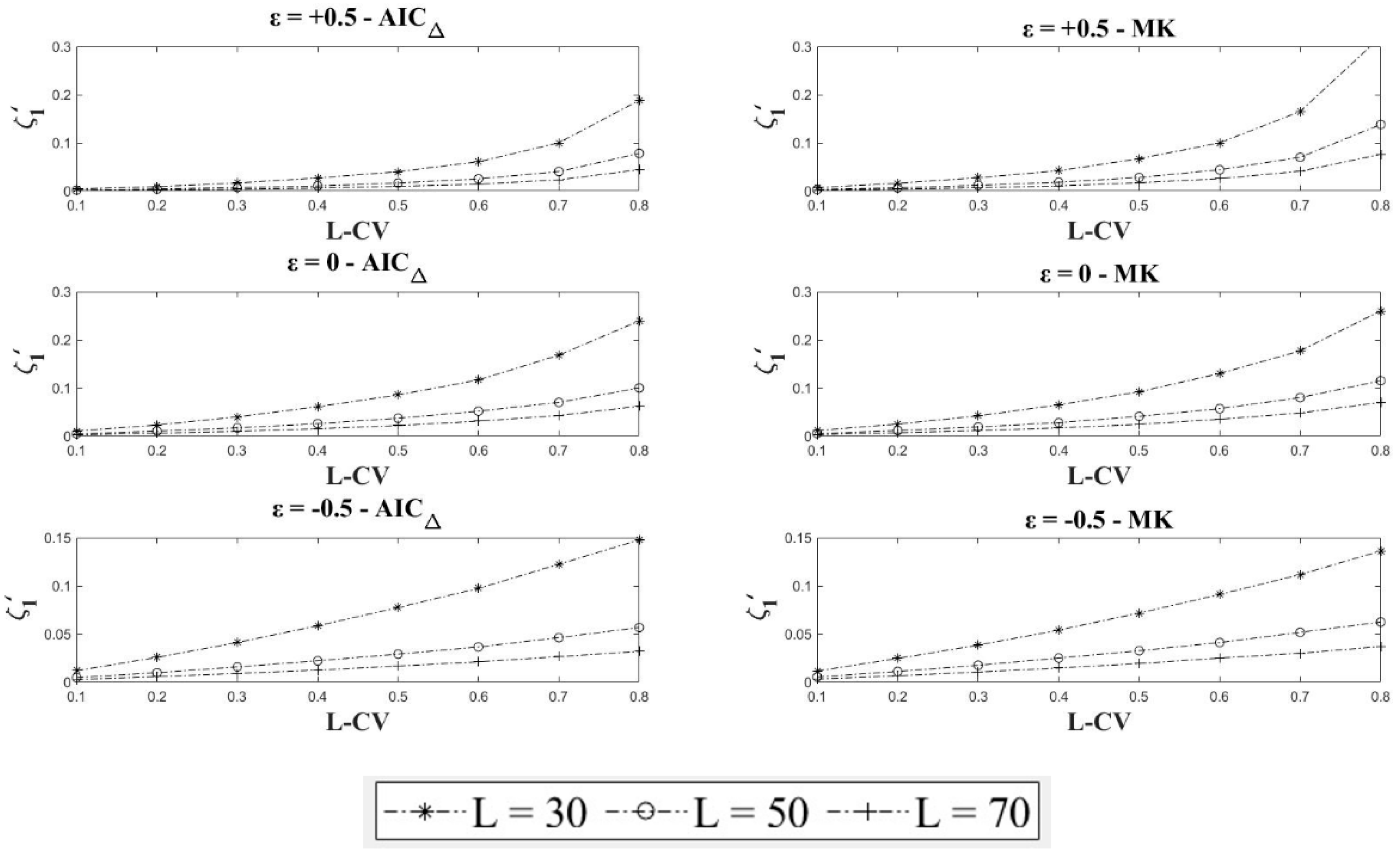
4.2. Sampling Variance of ${\zeta }_0$

A required task to apply the methodology suggested in this paper to real data is the evaluation of parameters of the parent distribution [${\zeta }_0,{\zeta }_1,\sigma ,\epsilon$]. Totaro et al. [14] already analyzed the sample variability and the empirical distribution obtained via Maximum Likelihood of parameters ${\zeta }_1^{}$, ε, and σ. Whilst this paper provides an extension of the range of considered values of σ, the results obtained here and the conclusions that were drawn are not different. Nevertheless, for the purpose of this paper, we focus on the sample variability of ${\zeta }_0$, which is crucial for obtaining rescaled values ${\zeta }_1^{\prime }$ and σ’. Results are obtained via Maximum Likelihood (ML) estimation of the four dimensionless parameters [${{\zeta }^{\prime }}_0,{{\zeta }^{\prime }}_1,{\sigma }^{\prime },\epsilon$] from generations of the nonstationary GEV parent distribution performed in the Monte Carlo experiment. Hence, generations are all characterized by ${{\zeta }^{\prime }}_0=1$ and different values of ${{\zeta }^{\prime }}_1,{\sigma }^{\prime }$, and $\epsilon$. Only results for the shorter considered sample length (L = 30) are reported for brevity. Figure 4 shows that the empirical distributions of the ML estimate of ${{\zeta }^{\prime }}_0$ (ML- ${{\zeta }^{\prime }}_0$) are generally unbiased and independent on the trend value ${{\zeta }^{\prime }}_1$. The estimator efficiency decreases with increasing L-CV for all $\epsilon$ values. The sample-variability of ${{\zeta }^{\prime }}_0$ can be analyzed also in Figure 5 where the standard deviation of the ML estimate of ${{\zeta }^{\prime }}_0$ is reported. The three subplots highlight that for upper-bounded GEV and EV1 the sample variability ${{\zeta }^{\prime }}_0$ is affected by L-CV but is independent of ${{\zeta }^{\prime }}_1$. Nevertheless, results relative to the heavy-tailed GEV (ε = +0.5) show that for the highest L-CV value (0.8) the sample variability of ${{\zeta }^{\prime }}_0$ sharply increases for series characterized by negative trend values lower than −0.04 and positive trend values higher than about +0.045. Such evidence suggests that the efficiency of the ML estimator remains the same than for the stationary case (${{\zeta }^{\prime }}_1=0$) for a wide range of parameter values in the upper-bounded GEV and EV1, while for heavy-tailed GEV with also high L-CV and trend values close to ±5% per year, estimators other than ML should be used.

4.3. Discussion

Salas and Obeysekera [19], exploiting the nonstationary GEV formulation provided by Coles [34], suggested that environment and climate change may affect the probability distribution of environmental variables by shifting in time the position parameter of the probability function (and possibly affecting also other distribution features, such as scale and shape parameters) from low to higher frequency. They showed that the presence of a positive trend in the position and scale parameters of the parent distribution may heavily affect the design standard of a built structure, such as a levee (floods), a bridge (wind speed), or other structural defenses like coastal protection structures and harbor breakwaters. As an example, depending on the values of observed trends, a structure designed (in stationary condition) for a 100-year return period, could face an expected waiting time [70] of the next exceedance of fewer than 30 years (see also Du et al. [71]).

In the environmental sciences and related applications, the detection of stationarity or nonstationarity for a selected time series is usually performed by using nonparametric tests available in the literature (e.g., Mann–Kendall or CUSUM test). Recent studies (e.g., Totaro et al. [14]) show that this kind of analysis may exploit well-developed model selection tools (e.g., the Akaike Information Criterion); this implies the use of parametric methods, and raises issues related to parameter estimation of a probability distribution, in stationary and nonstationary conditions. In particular, this paper confirms results obtained by Totaro et al. [14] and extends their analysis to wider ranges of the GEV shape and scale parameters, depending on L-skewness and L-CV values typical of physical variables of interest for climate change assessment.

The power value of AIC_Δ and MK tests is reported for different sample sizes and three GEV special cases: upper-bounded, EV1, and heavy-tailed. A strong dependence of power on L-CV is found in all cases and values below the conventional threshold 0.8 are found for ranges of ${\zeta }_1^{\prime }$, which in many cases exceeds the limits of our analysis i.e., ±5% per year. For such cases, we have extended the range of ${\zeta }_1^{\prime }$ up to values that allow the reaching of an acceptable power value. As a result of these analyses, we provide in Figure 3 the minimum absolute value of ${\zeta }_1^{\prime }$ which could be detected with acceptable power value (greater than 0.8). Such a threshold value of the trend depends on the used test and also on the L-CV and sample length L of the observed series. The same figure may be used to figure out which is the minimum sample length needed to perform trend analysis for known values of ${\zeta }_1^{\prime }$ and L-CV.

The analysis of sample variability of the position parameter shows that the ML procedure usually suggested for evaluating parameters of the nonstationary GEV distribution, in the explored range of parameter values and sample lengths, performs as well as for the stationary case (${\zeta }_1^{\prime }=0$) in both the upper-bounded and the EV1 special cases of GEV. For heavy-tailed GEV, with L-CV higher than 0.5, the sample variability sharply grows for trend coefficients approaching ±5% per year. On the other hand, the ML bias is independent of the trend coefficient in the entire examined trend coefficient range and for all the used parameter sets.

Results of this study, after Vogel et al. [10], suggest that procedures for assessing the statistical significance of observed trends in real-world data should follow a recognized experimental design protocol aimed to guarantee a minimum level of test power or, otherwise, a numerical assessment of the test power should be provided through a properly designed numerical Monte Carlo experiment. This could contribute to understanding the complex change patterns often observed in time series all over the world (e.g., [72,73]) together with the increasing number of natural hazards and related losses observed by many studies (e.g., [74,75]). Relatively weak but important trends could be investigated, apart from the concept of statistical significance as provided by procedures based on the adoption of a stationary null hypothesis [13]. On the other hand, much more effort should be devoted to the estimation of the trend coefficient. As shown by Totaro et al. [14], the very high sample variability shown by this parameter, even if it is estimated using a non-parametric method such as the well-known Sen’s slope [76], may provide also a trend of a different sign (negative rather than positive or vice-versa) as an effect of high sample variability, for relatively short samples (30 years).

In order to exploit the parametric approach within an accepted framework for risk assessment, other important steps are required. The use of nonstationary distributions, such as the Rescaled GEV in Equation (14), raises the problem of estimating a four-parameter set from observed data. This task is not trivial, as was shown in Section 4 for the position parameter, and by Totaro et al. [14] for the trend coefficient, and the scale and shape parameters. Moreover, in real-world data, trends could be not linear, could also affect other parameters, and could be not homogeneous in a long period spanning for several decades. In principle, deterministic trends for future projections should be provided by suitable climate models according to specifically selected scenarios. In such a case, parametric procedures for trend detection on observed series could be useful to validate or select the climate models based on their runs on a reference period.

Such procedures are also of broad general interest since the recent occurrence of relevant natural disasters (such as floods, hurricanes, earthquakes, tsunamis) induced the scientific community to provide a deeper understanding of relationships between extreme events and new emerging risks, with particular focus on cascading multi-hazard effects [77,78,79]. In this framework, procedures of risk assessment accounting for environment and climate change may lead to recognizing new areas subject to risk. The evaluation of areas exposed to a potential hazard should be periodically revised, with the consequence that critical facilities and infrastructures that were assumed to be in a safe location could be re-considered exposed to risk.

5. Conclusions

In this paper, a parametric methodology based on the AIC is proposed, suitable for establishing whether the presence of a specified trend is detectable or not from a series of known characteristics. To this purpose, we introduced a GEV distributed variable rescaled by the position parameter.

We compared the performances of the parametric AIC_Δ test and non-parametric MK test, analyzing their power with reference to observed ranges of different hydrological extreme variables. With this aim, we scoped case studies found in the literature dealing with extensive databases of annual maximum series of precipitation, peak flow, and wind speed. Through Monte Carlo simulations, a sensitivity analysis of both tests’ power was carried out to parameters of the Rescaled GEV distributed variable, showing that power strongly depends on dimensionless parameters ε, L-CV, and ${\zeta }_{1,}^{\prime }$.

Results are of practical interest, and in particular, we provided a tool for evaluating if the length of an available sample series suffices in reaching a conventional power value, depending on the values of the parent distribution, in the hypothesis that only a linear trend on the position parameter occurs. Obviously, from a general point of view, other sources and types of nonstationarity also may occur and negatively affect test power.

This paper sheds more light on parametric and non-parametric approaches for assessing nonstationarity of climatic variables and highlights important drawbacks in both of them. Nevertheless, it also shows that through a parametric procedure, the evaluation of method performances is feasible. More effort is needed to develop powerful methodologies for the analysis of real data, accounting for many other sources of variability and nonstationarity affecting the climatic and environmental extreme processes.

References

1. Murphy, B.L. From interdisciplinary to inter-epistemological approaches: Confronting the challenges of integrated climate change research. Can. Geogr. 2011, 55, 490–509. [Google Scholar] [CrossRef]
2. Rineau, F.; Malina, R.; Beenaerts, N.; Arnauts, N.; Bardgett, R.D.; Berg, M.P.; Boerema, A.; Bruckers, L.; Clerinx, J.; Davin, E.L.; et al. Towards more predictive and interdisciplinary climate change ecosystem experiments. Nat. Clim. Chang. 2019, 9, 809–816. [Google Scholar] [CrossRef]
3. Metzger, M.J.; Leemans, R.; Schröter, D. A multidisciplinary multi-scale framework for assessing vulnerabilities to global change. Int. J. Appl. Earth Obs. Geoinf. 2005, 7, 253–267. [Google Scholar] [CrossRef]
4. Cagle, L.E.; Tillery, D. Climate change research across disciplines: The value and uses of multidisciplinary research reviews for technical communication. Tech. Commun. Q. 2015, 24, 147–163. [Google Scholar] [CrossRef]
5. Blöschl, G.; Montanari, A. Climate change impacts-throwing the dice? Hydrol. Process. 2010, 24, 374–381. [Google Scholar] [CrossRef]
6. Donat, M.G.; Lowry, A.L.; Alexander, L.V.; O’Gorman, P.A.; Maher, N. More extreme precipitation in the world’ s dry and wet regions. Nat. Clim. Chang. 2016, 6, 508–513. [Google Scholar] [CrossRef]
7. Kundzewicz, Z.W.; Robson, A.J. Change detection in hydrological records—A review of the methodology. Hydrol. Sci. J. 2004, 49, 7–19. [Google Scholar] [CrossRef]
8. Cohen, J. The earth is round (p < 0.05). Am. Psychol. 1994. [Google Scholar] [CrossRef]
9. Serinaldi, F.; Kilsby, C.G.; Lombardo, F. Untenable nonstationarity: An assessment of the fitness for purpose of trend tests in hydrology. Adv. Water Resour. 2018, 111, 132–155. [Google Scholar] [CrossRef]
10. Vogel, R.M.; Rosner, A.; Kirshen, P.H. Brief Communication: Likelihood of societal preparedness for global change: Trend detection. Nat. Hazards Earth Syst. Sci. 2013, 13, 1773–1778. [Google Scholar] [CrossRef] [Green Version]
11. Milly, P.C.D.; Betancourt, J.; Falkenmark, M.; Hirsch, R.M.; Kundzewicz, Z.W.; Lettenmaier, D.P.; Stouffer, R.J.; Dettinger, M.D.; Krysanova, V. On Critiques of “stationarity is Dead: Whither Water Management?”. Water Resour. Res. 2015, 7785–7789. [Google Scholar] [CrossRef] [Green Version]
12. Beven, K. Facets of uncertainty: Epistemic uncertainty, non-stationarity, likelihood, hypothesis testing, and communication. Hydrol. Sci. J. 2016, 61, 1652–1665. [Google Scholar] [CrossRef] [Green Version]
13. Wasserstein, R.L.; Schirm, A.L.; Lazar, N.A. Moving to a World Beyond “p < 0.05.”. Am. Stat. 2019, 73, 1–19. [Google Scholar] [CrossRef] [Green Version]
14. Totaro, V.; Gioia, A.; Iacobellis, V. Numerical investigation on the power of parametric and nonparametric tests for trend detection in annual maximum series. Hydrol. Earth Syst. Sci. 2020, 24, 473–488. [Google Scholar] [CrossRef] [Green Version]
15. Yue, S.; Pilon, P.; Cavadias, G. Power of the Mann-Kendall and Spearman’s rho tests for detecting monotonic trends in hydrological series. J. Hydrol. 2002, 259, 254–271. [Google Scholar] [CrossRef]
16. Wang, F.; Shao, W.; Yu, H.; Kan, G.; He, X.; Zhang, D.; Ren, M.; Wang, G. Re-evaluation of the Power of the Mann-Kendall Test for Detecting Monotonic Trends in Hydrometeorological Time Series. Front. Earth Sci. 2020, 8. [Google Scholar] [CrossRef]
17. Montanari, A.; Koutsoyiannis, D. Modeling and mitigating natural hazards: Stationarity is immortal! Water Resour. Res. 2014, 50, 9748–9756. [Google Scholar] [CrossRef]
18. Serinaldi, F.; Kilsby, C.G. Stationarity is undead: Uncertainty dominates the distribution of extremes. Adv. Water Resour. 2015, 77, 17–36. [Google Scholar] [CrossRef] [Green Version]
19. Salas, J.D.; Obeysekera, J. Revisiting the Concepts of Return Period and Risk for Nonstationary Hydrologic Extreme Events. J. Hydrol. Eng. 2014, 19, 554–568. [Google Scholar] [CrossRef] [Green Version]
20. Yohe, G.W.; Lasco, R.D.; Ahmad, Q.K.; Arnell, N.W.; Cohen, S.J.; Hope, C.; Janetos, A.C.; Perez, R.T. Perspectives on climate change and sustainability. Climate Change 2007: Impacts, Adaptation and Vulnerability. Contribution of Working Group II to the Fourth Assessment Report of the Intergovernmental Panel on Climate Change; Parry, M.L., Canziani, O.F., Palutikof, J.P., van der Linden, P.J., Hanson, C.E., Eds.; Cambridge University Press: Cambridge, UK, 2007; pp. 811–841. [Google Scholar]
21. Stedinger, J.R.; Vogel, R.M.; Foufoula-Georgiou, E. Frequency analysis of extreme events. In Handbook of Hydrology; Maidment, D.R., Ed.; McGraw-Hill: New York, NY, USA, 1993; pp. 18.1–18.68. [Google Scholar]
22. Lieber, R.L. Statistical significance and statistical power in hypothesis testing. J. Orthop. Res. 1990, 8, 304–309. [Google Scholar] [CrossRef]
23. Cohen, J. A power primer. Psychol. Bull. 1992, 112, 155–159. [Google Scholar] [CrossRef] [PubMed]
24. Hosking, J.R.M. L-Moments: Analysis and Estimation of Distributions Using Linear Combinations of Order Statistics. J. R. Stat. Soc. Ser. B 1990, 52, 105–124. [Google Scholar] [CrossRef]
25. Mann, H.B. Nonparametric Tests Against Trend. Econometrica 1945, 13, 245–259. [Google Scholar] [CrossRef]
26. Kendall, M.G. Rank Correlation Methods; Griffin: London, UK, 1975; ISBN 978-0-85264-199-6. [Google Scholar]
27. Akaike, H. A New Look at the Statistical Model Identification. IEEE Trans. Autom. Control 1974, 19, 716–723. [Google Scholar] [CrossRef]
28. Laio, F.; Di Baldassarre, G.; Montanari, A. Model selection techniques for the frequency analysis of hydrological extremes. Water Resour. Res. 2009. [Google Scholar] [CrossRef]
29. Iacobellis, V.; Fiorentino, M.; Gioia, A.; Manfreda, S. Best fit and selection of theoretical flood frequency distributions based on different runoff generation mechanisms. Water (Switzerland) 2010, 2, 239–256. [Google Scholar] [CrossRef]
30. Burnham, K.P.; Anderson, D.R.; Huyvaert, K.P. AIC model selection and multimodel inference in behavioral ecology: Some background, observations, and comparisons. Behav. Ecol. Sociobiol. 2011, 65, 23–35. [Google Scholar] [CrossRef]
31. Burnham, K.P.; Anderson, D.R. Multimodel inference: Understanding AIC and BIC in model selection. Sociol. Methods Res. 2004, 33, 261–304. [Google Scholar] [CrossRef]
32. Jenkinson, A.F. The frequency distribution of the annual maximum (or minimum) values of meteorological elements. Q. J. R. Meteorol. Soc. 1955, 81, 158–171. [Google Scholar] [CrossRef]
33. Hosking, J.R.M.; Wallis, J.R. Regional Frequency Analysis; Cambridge University Press: Cambridge, UK, 1997. [Google Scholar]
34. Coles, S. An Introduction to Statistical Modeling of Extreme Values; Springer: London, UK, 2001. [Google Scholar]
35. Gilleland, E.; Katz, R.W. ExtRemes 2.0: An extreme value analysis package in R. J. Stat. Softw. 2016, 72, 1–39. [Google Scholar] [CrossRef] [Green Version]
36. Fowler, H.J.; Kilsby, C.G. A regional frequency analysis of United Kingdom extreme rainfall from 1961 to 2000. Int. J. Climatol. 2003, 23, 1313–1334. [Google Scholar] [CrossRef]
37. Lee, S.H.; Maeng, S.J. Frequency analysis of extreme rainfall using L-moment. Irrig. Drain. 2003, 52, 219–230. [Google Scholar] [CrossRef]
38. Ngongondo, C.S.; Xu, C.Y.; Tallaksen, L.M.; Alemaw, B.; Chirwa, T. Regional frequency analysis of rainfall extremes in Southern Malawi using the index rainfall and L-moments approaches. Stoch. Environ. Res. Risk Assess. 2011, 25, 939–955. [Google Scholar] [CrossRef] [Green Version]
39. Wan Zin, W.Z.; Jemain, A.A.; Ibrahim, K. The best fitting distribution of annual maximum rainfall in Peninsular Malaysia based on methods of L-moment and LQ-moment. Theor. Appl. Climatol. 2009, 96, 337–344. [Google Scholar] [CrossRef]
40. Papalexiou, S.M.; Koutsoyiannis, D. Battle of extreme value distributions: A global survey on extreme daily rainfall. Water Resour. Res. 2013, 49, 187–201. [Google Scholar] [CrossRef]
41. Abolverdi, J.; Khalili, D. Development of Regional Rainfall Annual Maxima for Southwestern Iran by L-Moments. Water Resour. Manag. 2010, 24, 2501–2526. [Google Scholar] [CrossRef]
42. Alahmadi, F.S. Regional Rainfall Frequency Analysis By L-Moments Approach For Madina Region, Saudi Arabia. Int. J. Eng. Res. Dev. 2017, 13, 39–48. [Google Scholar]
43. Yurekli, K.; Modarres, R.; Ozturk, F. Regional daily maximum rainfall estimation for Cekerek Watershed by L-moments. Meteorol. Appl. 2009, 16, 435–444. [Google Scholar] [CrossRef]
44. Shahzadi, A.; Akhter, A.S.; Saf, B. Regional frequency analysis of annual maximum rainfall in monsoon region of pakistan using L-moments. Pak. J. Stat. Oper. Res. 2013, 9, 111–136. [Google Scholar] [CrossRef] [Green Version]
45. Zakaria, Z.A.; Shabri, A.; Ahmad, U.N. Regional Frequency Analysis of Extreme Rainfalls in the West Coast of Peninsular Malaysia using Partial L-Moments. Water Resour. Manag. 2012, 26, 4417–4433. [Google Scholar] [CrossRef]
46. Forestieri, A.; Lo Conti, F.; Blenkinsop, S.; Cannarozzo, M.; Fowler, H.J.; Noto, L.V. Regional frequency analysis of extreme rainfall in Sicily (Italy). Int. J. Climatol. 2018, 38, e698–e716. [Google Scholar] [CrossRef]
47. Abida, H.; Ellouze, M. Probability distribution of flood flows in Tunisia. Hydrol. Earth Syst. Sci. 2008, 12, 703–714. [Google Scholar] [CrossRef] [Green Version]
48. Glaves, R.; Waylen, P.R. Regional flood frequency analysis in Southern Ontario using L-moments. Can. Geogr. 1997, 41, 178–193. [Google Scholar] [CrossRef]
49. Salinas, J.L.; Castellarin, A.; Viglione, A.; Kohnová, S.; Kjeldsen, T.R. Regional parent flood frequency distributions in Europe—Part 1: Is the GEV model suitable as a pan-European parent? Hydrol. Earth Syst. Sci. 2014, 18, 4381–4389. [Google Scholar] [CrossRef] [Green Version]
50. Vogel, R.M.; Thomas, W.O.; McMahon, T.A. Flood-flow frequency model selection in southwestern United States. J. Water Resour. Plan. Manag. 1993, 119, 353–366. [Google Scholar] [CrossRef] [Green Version]
51. Drissia, T.K.; Jothiprakash, V.; Anitha, A.B. Flood Frequency Analysis Using L Moments: A Comparison between At-Site and Regional Approach. Water Resour. Manag. 2019, 33, 1013–1037. [Google Scholar] [CrossRef]
52. Hussain, Z.; Pasha, G.R. Regional flood frequency analysis of the seven sites of Punjab, Pakistan, using L-moments. Water Resour. Manag. 2009, 23, 1917–1933. [Google Scholar] [CrossRef]
53. Meshgi, A.; Khalili, D. Comprehensive evaluation of regional flood frequency analysis by L- and LH-moments. I. A re-visit to regional homogeneity. Stoch. Environ. Res. Risk Assess. 2009, 23, 119–135. [Google Scholar] [CrossRef]
54. Noto, L.V.; La Loggia, G. Use of L-moments approach for regional flood frequency analysis in Sicily, Italy. Water Resour. Manag. 2009, 23, 2207–2229. [Google Scholar] [CrossRef]
55. Pearson, C.P. New Zealand regional flood frequency analysis using L-moments. J. Hydrol. (N. Z.) 1991, 30, 53–64. [Google Scholar]
56. Salinas, J.L.; Castellarin, A.; Kohnová, S.; Kjeldsen, T.R. Regional parent flood frequency distributions in Europe—Part 2: Climate and scale controls. Hydrol. Earth Syst. Sci. 2014, 18, 4391–4401. [Google Scholar] [CrossRef] [Green Version]
57. Seckin, N.; Haktanir, T.; Yurtal, R. Flood frequency analysis of Turkey using L-moments method. Hydrol. Process. 2011, 25, 3499–3505. [Google Scholar] [CrossRef]
58. Vogel, R.M.; McMahon, T.A.; Chiew, F.H.S. Floodflow frequency model selection in Australia. J. Hydrol. 1993, 146, 421–449. [Google Scholar] [CrossRef]
59. Jung, C.; Schindler, D. Wind speed distribution selection—A review of recent development and progress. Renew. Sustain. Energy Rev. 2019, 114, 109290. [Google Scholar] [CrossRef]
60. Morgan, E.C.; Lackner, M.; Vogel, R.M.; Baise, L.G. Probability distributions for offshore wind speeds. Energy Convers. Manag. 2011, 52, 15–26. [Google Scholar] [CrossRef]
61. Palutikof, J.P.; Brabson, B.B.; Lister, D.H.; Adcock, S.T. A review of methods to calculate extreme wind speeds. Meteorol. Appl. 1999, 6, 119–132. [Google Scholar] [CrossRef]
62. Fawad, M.; Yan, T.; Chen, L.; Huang, K.; Singh, V.P. Multiparameter probability distributions for at-site frequency analysis of annual maximum wind speed with L-Moments for parameter estimation. Energy 2019, 181, 724–737. [Google Scholar] [CrossRef]
63. Goel, N.K.; Burn, D.H.; Pandey, M.D.; An, Y. Wind quantile estimation using a pooled frequency analysis approach. J. Wind Eng. Ind. Aerodyn. 2004, 92, 509–528. [Google Scholar] [CrossRef]
64. Hong, H.P.; Ye, W. Estimating extreme wind speed based on regional frequency analysis. Struct. Saf. 2014, 47, 67–77. [Google Scholar] [CrossRef]
65. MacKenzie, C.A.; Winterstein, S.R. Comparing L-moments and conventional moments to model current speeds in the North Sea. In Proceedings of the 61st Annual IIE Conference and Expo Proceedings, Reno, NV, USA, 24 May 2011. [Google Scholar]
66. Pandey, M.D.; Van Gelder, P.H.A.J.M.; Vrijling, J.K. The estimation of extreme quantiles of wind velocity using L-moments in the peaks-over-threshold approach. Struct. Saf. 2001, 23, 179–192. [Google Scholar] [CrossRef]
67. Hundecha, Y.; St-Hilaire, A.; Ouarda, T.B.M.J.; El Adlouni, S.; Gachon, P. A nonstationary extreme value analysis for the assessment of changes in extreme annual wind speed over the gulf of St. Lawrence Canada. J. Appl. Meteorol. Climatol. 2008, 47, 2745–2759. [Google Scholar] [CrossRef]
68. Fawad, M.; Ahmad, I.; Nadeem, F.A.; Yan, T.; Abbas, A. Estimation of wind speed using regional frequency analysis based on linear-moments. Int. J. Climatol. 2018, 38, 4431–4444. [Google Scholar] [CrossRef]
69. Modarres, R. Regional maximum wind speed frequency analysis for the arid and semi-arid regions of Iran. J. Arid Environ. 2008, 72, 1329–1342. [Google Scholar] [CrossRef]
70. Olsen, J.R.; Lambert, J.H.; Haimes, Y.Y. Risk of extreme events under nonstationary conditions. Risk Anal. 1998, 18, 497–510. [Google Scholar] [CrossRef]
71. Du, T.; Xiong, L.; Xu, C.Y.; Gippel, C.J.; Guo, S.; Liu, P. Return period and risk analysis of nonstationary low-flow series under climate change. J. Hydrol. 2015, 527, 234–250. [Google Scholar] [CrossRef] [Green Version]
72. Do, H.X.; Westra, S.; Leonard, M. A global-scale investigation of trends in annual maximum streamflow. J. Hydrol. 2017, 552, 28–43. [Google Scholar] [CrossRef]
73. Kundzewicz, Z.W.; Kanae, S.; Seneviratne, S.I.; Handmer, J.; Nicholls, N.; Peduzzi, P.; Mechler, R.; Bouwer, L.M.; Arnell, N.; Mach, K.; et al. Flood risk and climate change: Global and regional perspectives. Hydrol. Sci. J. 2014, 59, 1–28. [Google Scholar] [CrossRef] [Green Version]
74. Wallemacq, P.; Below, R. The Human Cost of Natural Disasters: A Global Perspective; Centre for Research on the Epidemiology of Disaster: Brussels, Belgium, 2015. [Google Scholar]
75. Formetta, G.; Feyen, L. Empirical evidence of declining global vulnerability to climate-related hazards. Glob. Environ. Chang. 2019, 57. [Google Scholar] [CrossRef]
76. Sen, P.K. Estimates of the Regression Coefficient Based on Kendall’s Tau. J. Am. Stat. Assoc. 1968, 63, 1379–1389. [Google Scholar] [CrossRef]
77. Forzieri, G.; Bianchi, A.; Silva, F.P.; Herrerad, M.A.M.; Lebloise, A.; Lavallec, C.; Jeroen, C.J.H.; Aertsf, J.C.J.H.; Feyenh, L. Escalating impacts of climate extremes on critical infrastructures in Europe. Glob. Environ. Chang. 2018, 48, 97–107. [Google Scholar] [CrossRef]
78. Gill, J.C.; Malamud, B.D. Hazard interactions and interaction networks (cascades) within multi-hazard methodologies. Earth Syst. Dyn. 2016, 7. [Google Scholar] [CrossRef] [Green Version]
79. Krausmann, E.; Cruz, A.M.; Salzano, E. Natech Risk Assessment and Management: Reducing the Risk of Natural-Hazard Impact on Hazardous Installations; Elsevier: Amsterdam, The Netherlands, 2016; ISBN 9780128038796. [Google Scholar]
80. Yue, S.; Pilon, P.; Phinney, B.; Cavadias, G. The influence of autocorrelation on the ability to detect trend in hydrological series. Hydrol. Process. 2002, 16, 1807–1829. [Google Scholar] [CrossRef]
Figure 1. Power value of Akaike Information Criterion difference (AICΔ) test vs. trend coefficient ζ 1   , for different ε and L values.
Sustainability 12 03889 g001
Figure 2. Power value of Mann–Kendall (MK) test vs. trend coefficient ζ 1 for different ε and L values.
Sustainability 12 03889 g002
Figure 3. Minimum trend coefficient | ζ 1 | required to obtain power ≥0.8 vs. L-CV values for the AICΔ (left column) and MK (right column) tests and for different ε values.
Sustainability 12 03889 g003
Figure 4. Sample distribution of ML- ζ 0 for L = 30 and different values of ε and L-CV.
Sustainability 12 03889 g004
Figure 5. Standard deviation of M L ζ 0 for L=30 and different values of ε and L-CV.
Sustainability 12 03889 g005