Cost Modeling and Evaluation of Direct Metal Laser Sintering with Integrated Dynamic Process Planning

Abstract

Additive manufacturing technologies have been adopted in a wide range of industries such as automotive, aerospace, and consumer products. Currently, additive manufacturing is mainly used for small-scale, low volume productions due to its limitations such as high unit cost. To enhance the scalability of additive manufacturing, it is critical to evaluate and preferably reduce the cost of adopting additive manufacturing for production. The current literature on additive manufacturing cost mainly adopts empirical approaches and does not sufficiently explore the cost-saving potentials enabled by leveraging different process planning algorithms. In this article, a mathematical cost model is established to quantify the different cost components in the direct metal laser sintering process, and it is applicable for evaluating the cost performance when adopting dynamic process planning with different layer-wise process parameters. The case study results indicate that 12.73% of the total production cost could be potentially reduced when applying the proposed dynamic process planning algorithm based on the complexity level of geometries. In addition, the sensitivity analysis results suggest that the raw material price and the overhead cost are the two key cost drivers in the current additive manufacturing market.

1. Introduction

In recent years, public interest in innovating and improving additive manufacturing (AM) technologies has been immensely growing since the first emergence in the 1970s. Compared with traditional subtractive manufacturing processes, AM has shown to have great potentials for enhanced manufacturing complexity, reduced production time and cost, as well as an increased level of customization [1]. It is estimated that with the current growth rate, the direct market of AM will reach USD100 to billion by 2025 [2]. Owing to these superior advantages, AM technologies have been adopted in various industries including aerospace [3,4,5], medical [6,7], consumer goods [8], automotive [9,10], etc. For these different applications, a wide range of raw materials have been used such as metal, ceramics, glass, paper, wood, cement, graphene, and even living cells [11]. Currently, several AM processes with high deposition rates have been used in high production volumes [12,13], but most AM applications are still limited to that of small- to medium-sized productions, due to the relatively low production speed, unsatisfactory fabrication quality, and relatively high cost per part (especially for smaller production volume). The production cost, as one of the critical aspects of sustainability (along with environmental and social sustainability), plays a guiding role in the evaluation of a new manufacturing process [14]. In the current literature, cost assessments have been conducted for different AM processes [15,16,17,18,19,20,21,22,23,24,25,26,27] including fused filament fabrication (FFF) [18], mask image projection-based stereolithography [23], fused deposition modeling [19], light-directed electrophoretic deposition [28], inkjet printing [29], multijet printing [30], laminated object manufacturing [31], and electron beam manufacturing [32], etc.

Metal-based AM processes have been dominating the AM market as the investment in metal-based three-dimensional (3D) printing has been growing significantly in the past years. According to the latest Wohlers Report, the worldwide revenue of metal AM grew at a rate of 41.9% in 2019 [15]. Metal AM technologies have been favored in different application domains. For example, GE Aviation has applied the laser-based AM technique to fabricate critical components on LEAP jet engines, such as fuel nuzzle tip, engine inducer, and combustor mixer [33]. Siemens has employed the direct metal laser sintering (DMLS) to fabricate gas turbine blades that can be used in production of power generation [34]. To further increase the market share of the metal AM market, it is necessary to evaluate and preferably reduce the overall cost. In the current literature, studies on cost evaluation have been performed for metal-based AM processes [1,16,18,19,20,21,22,26,35,36,37,38], and they suggest great opportunities for saving production costs by adjusting production plans such as changing the selection of process parameters [1,21]. The majority of these cost studies do not rely on mathematical cost models, and they are mostly case specific, which limits the applicability of their analysis results, as well as the potential for cost optimization.

In the current literature, some cost models have been established for metal-based AM processes [20,21,22,26,37,38] for different research goals such as quantifying the production cost of different part geometries and batch sizes [20], comparing the support cost using different overhang angles and support structures [21], exploring the opportunity for reducing the cost for different building volumes [26], comparing the cost of traditional CNC and metal-based AM [22], and applying topology optimization with cost constraints [38]. While these cost models provide useful insights into understanding the different cost components in metal-based AM, most of them are based on a constant selection of process parameters within one batch, in other words, they consider the values of process parameters to be constant during the fabrication. Dynamic process planning, which has been widely adopted in traditional manufacturing processes [39,40,41], can help save production time, reduce cost, and improve the overall productivity [37]. In the DMLS process, the selection of values for process parameters such as laser power, scanning speed, and hatching distance is likely to affect the production cost, as well as fabrication quality [42]. Limited by machine specifications, these process parameters usually can be altered within feasible ranges [43]. The selection of these values is jointly determined by the desired quality and feasible production time (cost), with the potential for adopting different values of process parameters for different portions of the fabrication (in build direction) to reduce the cost while ensuring fabrication quality. In the current literature, research on reducing the production cost by leveraging dynamic production planning is rarely conducted.

To fill the knowledge gap, a comprehensive cost model with an integrated dynamic process planning algorithm is established for the DMLS process. The layer-wise process parameters are selected based on the geometry complexity for the purpose of time and cost saving. Four case studies are conducted to investigate the performance of the proposed model and the dynamic process planning algorithm. The results from this paper would not assist AM manufacturers to improve their efficiency but could aid AM decision-makers towards cost-effective production planning and further advancement in AM. The remainder of this article is organized as follows: In Section 2, the DMLS process is illustrated, followed by the established cost model and the dynamic production planning algorithm; in Section 3, case studies are performed, including model evaluation, analysis of dynamic process settings, and sensitivity analysis; in Section 4, we discuss the conclusions and future work of this research.

2. Methodologies

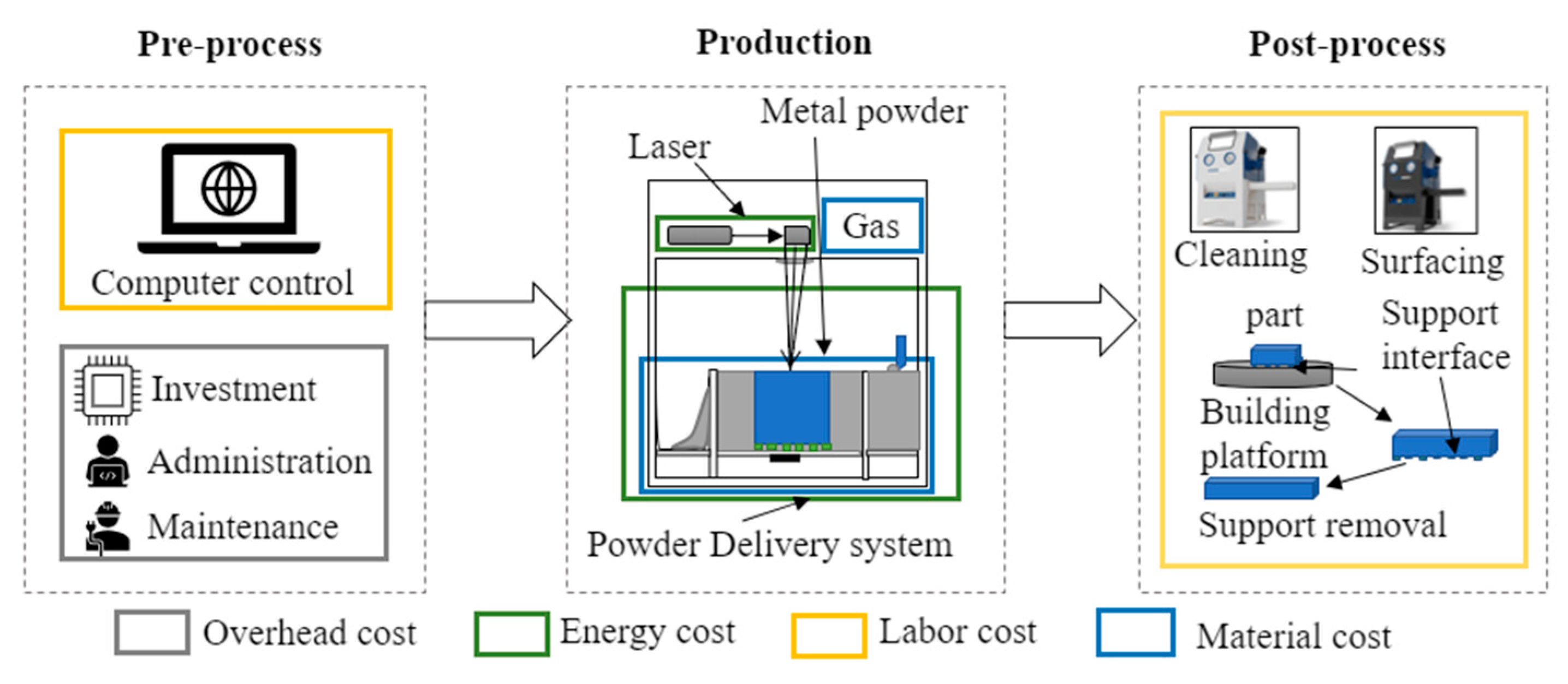
2.1. Illustration of the Direct Metal Laser Sintering Process

As one of the most popular metal-based AM technologies, the DMLS process projects a high-power laser beam onto a powder bed and fuses the atomized fine particles to create a solid structure layer-by-layer [44]. As illustrated in Figure 1, the production process can be categorized into three stages, i.e., the preprocessing stage, the production stage, and the postprocessing stage. During the preprocessing stage, the 3D geometry information is generated by designers and fed into the control software of the DMLS machine. The DMLS machine is set up with the materials and protective gas in the preprocessing stage. In practice, maintenance activities (including cleaning, component replacement, etc.) are conducted regularly to maintain the process reliability and stability. In the production stage, metal powders are delivered by a powder delivery system to the build platform, where a part is fabricated. The platform is installed in a chamber that is filled with protective gas [44]. During the fabrication process, the protective gas is delivered into the chamber at a steady rate. A roller is used to spread the powders onto the build platform. During the part fabrication, a high-power laser, which is controlled by a scanning mirror through changing its refection direction, is used to melt and fuse metallic powder at the platform layer-by-layer [45]. When the sintered metal powder is cooled down, the fabrication of a layer is completed. After the fabrication of each layer, the used powders are collected for recycling. During the postprocessing stage, the fabricated parts usually undergo several different steps necessary to further improve the finished quality, such as cleaning, hardening or curing, surface finishing, and coloring [43].

During the three stages of DMLS, different cost components occur. The total fabrication cost consists of overhead cost, energy cost, labor cost, and material cost. The overhead cost includes machine and software investment, administration, and maintenance, and it mainly occurs during the preprocessing stage. The energy cost covers the electricity cost caused by the laser device and the powder delivery system, and it mainly occurs during the production stage. The labor cost occurs in the labor-involved activities during the preprocessing phase as well as the postprocess phase. These postprocess procedures add to the time required to manufacture the parts [46]. The material cost is a collection of all the materials that are used in the manufacturing process.

2.2. Cost Modeling

To generate the total cost of the DMLS process, it is necessary to investigate the different components of the DMLS process. The total cost of the manufacturing process ($C_{Total}$) (USD) consists of the energy cost ($C_{energy}$), the labor cost ($C_{labor}$), the material cost ($C_{material}$), and the overhead cost ($C_{overhead}$). It can be formulated as follows:

$$C_{Total}=C_{energy}+C_{labor}+C_{material}+C_{overhead}$$

(1)

The unit cost per part in a batch with mixed geometry is determined by the mass and the geometry complexity of the part. The geometry complexity of each individual part needs to be calculated separately.

Let $i$ be the index of the part manufactured in a production batch, with mass $m_i$ and geometry complexity factor $f_{ge{o}_i}$. The cost for a specific part $k$ (USD) is estimated as follows:

$$C_{par{t}_k}=C_{Total}\times \frac{m_k\times f_{ge{o}_k}}{\sum m_i\times f_{ge{o}_i}}$$

(2)

In this equation, $m_i$ denotes the mass of the part $i$ (g), and $f_{ge{o}_i}$ represents the geometry complexity factor of the part $i$. The geometry complexity factor can be defined by different geometry information of the part.

2.2.1. Energy Consumption Cost

The energy consumption consists of several components, including the energy consumption during the production stage. The machine has some constant energy consumption components once it is started, such as cooling fans, monitoring units, etc. It also has some energy consumption related to the scanning time, such as the protective gas system, motor systems, laser units, etc. It is shown in Equation (3) as:

$$C_{energy}=(P_{const}\times t_{set}+{\displaystyle \sum }_j{E}_{laser,j}+(P_{mech}+P_{const})\times t_{scan}+((P_{recoat}+P_{mech})\times n_{layer}\times t_{layer})\times M_{energy}$$

(3)

Let $j$ be the index of the layer in the batch. $P_{const}$ represents the constant power consumption of the system, including control unit, fans, and heating systems, etc. (J/s), $t_{set}$ represents the time consumption before the building process, including preheating, self-calibration, etc. (s), $E_{laser,j}$ is the energy consumption of layer $j$ (J), $P_{mech}$ is the power of the nozzle motor system (J/s), $P_{recoat}$ denotes the power of the recoating system (J/s), $n_{layer}$ denotes the total number of layers, $t_{layer}$ represents the fixed recoating time for each layer (s), and $M_{energy}$ represents the monetary price of the energy (USD/J).

The energy consumption of layer $j$ can be estimated as:

$$E_{laser,j}={{\displaystyle \int }}_{t_{0,j}}^{t_{0,j}+t_{scan,j}}{P}_{laser{}_j}dt, P_{laser{}_j}\in P_{laser}$$

(4)

In the equation, $t_{scan}$ stands for the total scanning time (s), $t_{0,j}$ denotes the starting scanning time in the layer $j$, and $t_{scan,j}$ is the total scanning time in the layer $j$.

The total scanning time can be formulated as follows:

$$t_{scan}={\displaystyle \sum }_j{t}_{scan,j}$$

(5)

$$t_{scan,j}={\displaystyle \int }\frac{1}{V_{scan{}_j}\times H_{d_j} }dS, S\in S_j, V_{scan{}_j}\in V_{scan}$$

(6)

In the equations, $V_{scan{}_j}$ represents the scanning speed at the layer $j$ (mm/s) and $H_{d_j}$ denotes the hatching distance at the layer $j$ (mm).

2.2.2. Labor Cost

Labor cost is mainly determined by the process with the interaction of labor forces. Note it is assumed that there is no human interaction during the manufacturing process of DMLS. It includes setup for the machine, operating software, maintenance, preprocessing, and postprocessing. The cost of labor can be formulated as follows:

$$C_{labor}=\left(t_{setup}+t_{operating}+t_{pre-pro}+t_{post-pro}\right)\times M_{labor}$$

(7)

In this equation, $t_{setup}$ represents the setup time for the machine (h), $t_{operating}$ denotes the operating time for the machine (h), $t_{pre-pro}$ represents the preprocessing time (h), $t_{post-pro}$ represents the postprocessing time (h), and $M_{labor}$ denotes the hourly salary of the labor (USD/h).

2.2.3. Material Cost

The material cost primarily contains two sources, namely part material, and protective gas cost. The material cost can be formulated as proposed:

$$C_{material}=\frac{1}{{\alpha }_u}\times \left({\rho }_{metal}({\displaystyle \sum }_j{L}_j\times S_j+V_{support})\right)\times M_{metal}+V_{gas}\times t_{build}\times M_{gas}$$

(8)

In this equation, ${\alpha }_u$ denotes the utilization rate, ${\rho }_{metal}$ denotes the density of the metal material (g/mm³), $S_j$ represents the total area of in the layer $j$ (mm²), $M_{metal}$ represents the price of the metal material (USD/g), $V_{gas}$ denotes the gas release speed during the production (m³/h), $t_{build}$ represents the total production time (h), and $M_{gas}$ is the price of the protective gas (with the unit of volume) ($/L).

The total area in the layer $j$ can be estimated as follows:

$$S_j={\displaystyle \sum }_I{S}_{i,j}$$

(9)

$S_{i,j}$ denotes the area of the part $i$ in the layer $j$ (mm²).

2.2.4. Overhead

The overhead cost includes the machine preparation cost, the maintenance cost, and the administration cost. It is assumed that the machine has a limited life. The regular-period-based maintenance is executed. Additionally, a periodical administration for the machine is performed to ensure the stability of the machine. The overhead cost can be summarized as follows:

$$C_{overhead}=(M_{machine}/N_{life}+M_{maintenance}/N_{maintence}+M_{administration}/N_{administration})\times t_{build}$$

(10)

In this equation, $M_{machine}$ denotes the machine investment cost (USD) including hardware and software costs, $N_{life}$ denotes the life span of the machine (h), $M_{maintenance}$ denotes the maintenance cost (USD), $N_{maintence}$ represents the maintenance period (operation time between maintenances) (h), $M_{administration}$ represents the administration cost (USD), and $N_{administration}$ represents the administration period (h).

2.2.5. Geometry Complexity Factors

In the DMLS process, different process parameters, including laser power and scan speed, have been found to influence the production cost [22,25,47]. On the one hand, more laser power and slower scanning speed result in larger melt pools and fewer scanning operations. On the other hand, less laser power and faster scanning speed create thinner structures. According to the mechanism, if the process parameters in the planning strategy are decided by the geometry, significant time can be saved, and consequently, the total cost is reduced. The geometry complexity can be divided into two categories, i.e., layer-wise factor and volume-related factor. These two categories correspondingly influence layer-related and volume-related characteristics. The former category includes perimeter area ratio, isoperimetric ratio, and curvature statistics, etc. It represents the complexity of a specific layer of the part. The more complex a layer is, the more variation of the process parameters in the same layer will be required to better realize the layer-wise characteristics. The latter category includes fullness ratio, and three-dimensional bounding box ratio, etc. Volume-related factors influence volume-related characteristics. A weighed formulation of geometry complexities is introduced to decide the process parameters to achieve lower production costs. A set of process parameters $L$, $P_{laser}$, and $V_{scan}$ are decided by the geometry factors.

Geometry complexity can be defined with different geometry information. In this paper, layer-related geometry complexity is defined as the bounding box ratio of the layer. A layer may have multiple closed-loop polygons. The layer-wise geometry parameter of the layer $j$ in the part $i$ can be expressed as follows:

$$f_{ge{o}_{i,j}}=r_{bbox}$$

(11)

Volume-related factors are defined as the three-dimensional bounding box ratio. The volume-related complexity of the part $i$ can be expressed as follows:

$$f_{ge{o}_i}=\frac{{{\displaystyle \sum }}_j{L}_j\times S_{i,j}}{V_{bbox}}$$

(12)

In the equation, $V_{bbox}$ denotes the bounding box volume (mm³) of the three-dimensional models of the part $i$.

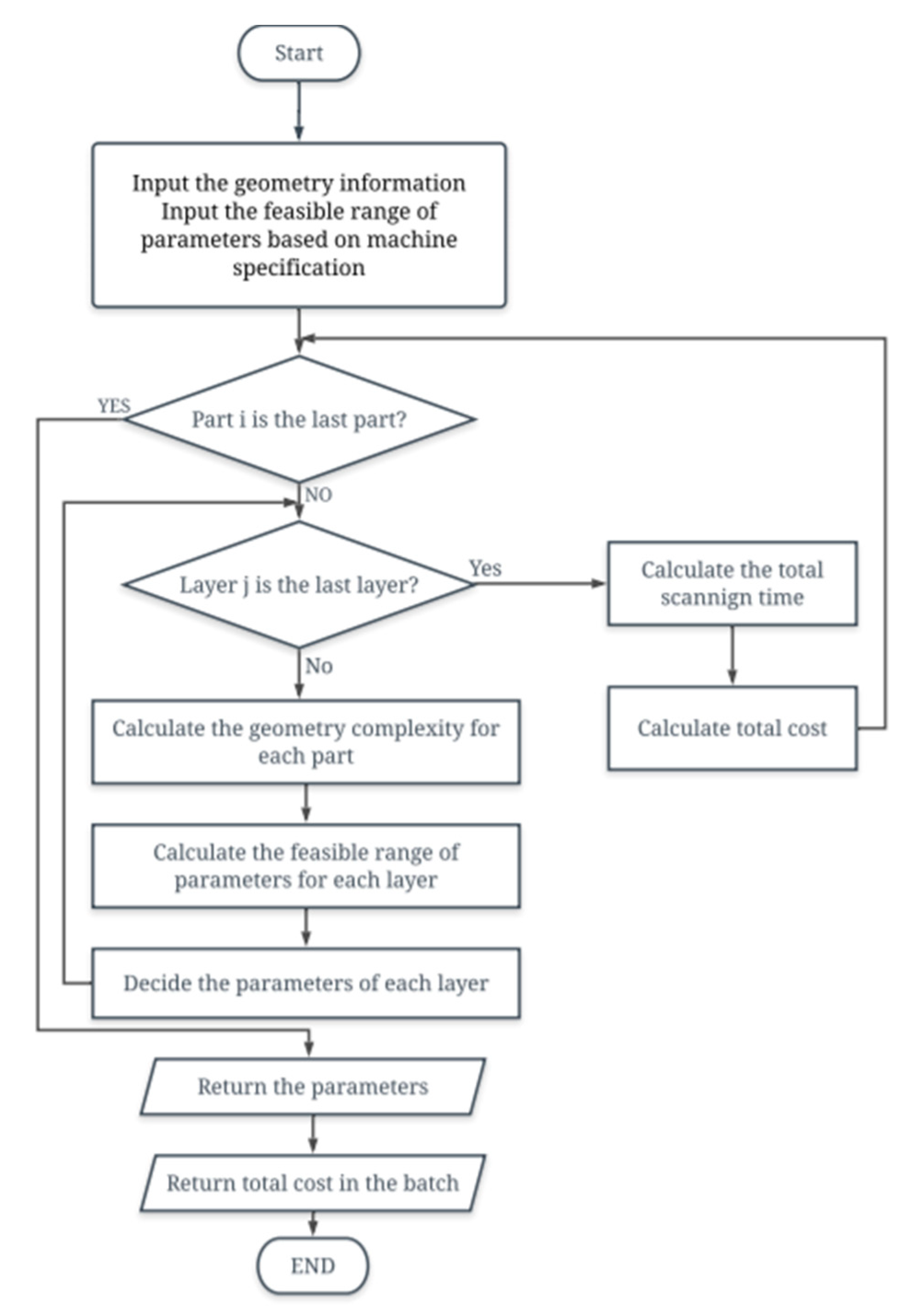
2.3. Process Planning Algorithm

To reduce the total cost of the DMLS process, a novel process planning algorithm is proposed to select parameters based on the geometry factors. The algorithm is demonstrated as follows: In detail, based on the part geometry information, a set of process parameters including laser speed, the hatching distance, and laser power is determined accordingly to decrease the total cost in the DMLS process.

Step 1 GET the part geometry information including volume-related factors $V_{bbox}$ and geometry complexity factors $f_{ge{o}_{i,j}}$ Step 2 GET the feasible ranges of changeable parameters $L_j$, $P_{laser{}_j}$, $V_{scan{}_j}$, and $H_{d_j}$ based on machine specification Step 3 FOR $i=1 : n_{Part}$   FOR $j=1 : n_{layer}$   CALCULATE the layer-wise geometry complexity $f_{ge{o}_i}$ based on the part geometry complexity factor $r_{bbox,i}$ for each part in the batch   CALCULATE the feasible range of parameters of $L_j$, $P_{laser{}_j}$, $V_{scan{}_j}$ according to $f_{ge{o}_{i,j}}$   CALCULATE scanning time for the layer $j$ as $t_{scan,j}$ according to the changeable parameters $L_j$, $P_{laser{}_j}$, $V_{scan{}_j}$     END LOOP     CALCULATE total scanning time $t_{scan}$     CALCULATE total cost $C_{Total}$ END LOOP Step 4 FIND a set of parameters $L$, $P_{laser}$, and $V_{scan}$ that reduce the total cost $C_{Total}$ Step 5 RETURN the solution with changeable parameters for each layer and total cost $C_{Total}$ Step 6 END

A flowchart describing the algorithm is shown in Figure 2.

3. Case Studies

In this section, four case studies are conducted to evaluate the performance of the established cost model, as well as the dynamic process planning algorithm. The first case study, in Section 3.1, is designed to compare the proposed model and the two existing models in the literature, in terms of calculating the total production cost for different types of materials. The second case study, in Section 3.2, is designed to explore using the proposed cost model for different production scenarios, i.e., production of one single geometry and production of a mixed batch of different geometries. The third case study, in Section 3.3, is designed to compare the calculated total production cost when using constant process parameters and the proposed dynamic process planning algorithm which is based on the geometry complexity. Finally, the sensitivity analysis, in Section 3.4, is designed to identify the key cost drivers in the current market that have a direct impact on the total production cost. To perform these case studies, some assumptions are adopted as shown in

Table 1. Cost model calculation assumptions.

Parameter	Value	Source
Machine rated power $P_{const}$	200 W	Technical data of EOS M290 [48]
Power of the motor system $P_{mech}$	1000 W
Power of the recoating system $P_{recoat}$	200 W
Gas release speed $V_{gas}$	28 m3/h
The life span of the machine $N_{life}$	3 years
Time of layer change $t_{layer}$	7.2 s	Estimated based on the practical operation
Unit price of the energy $M_{energy}$	$0.12/KWh	Averaged retail price of electricity in the residential sector, May 2020 [49]
Hourly salary of the labor $M_{labor}$	10.12 USD	Government data [50]
Material utilization rate ${\alpha }_u$	50%	Model assumption
Density of the material ${\rho }_{metal}$	4.41 mg/mm3	Material property [51]
Price of the material $M_{metal}$	$20.85/kg
Price of the protective gas $M_{gas}$	$0.14/cm3	The listed prices on the official website [48]
Machine investment $M_{machine}$	$600,000
Maintenance cost $C_{maintenance}$	$300
Administration cost $C_{administration}$	$35,000

, and they are applicable to all the case studies in this section.

3.1. Model Comparison with the Current Literature for Different Materials

In this case study, the proposed model is compared with the two existing cost models in the literature for different materials, i.e., 316L, AlSi10Mg, and Ti4Al6V. Similar sets of parameters are adopted as inputs in the proposed model and the existing models in the literature to calculate the total production costs, which are the outputs of this case study. The expected outcome of this case study is the comparison of model calculation results from the proposed model and the existing models in the literature.

Figure 3, Figure 4 and Figure 5 are the comparison results between the proposed model and the existing models in the literature [20,25]. Three metal are used to compare the cost calculation for the model proposed in this work, namely 316L, AlSi10Mg, and Ti4Al6V. According to the figures, the model in this work has close calculation results with the models in the literature. To compare the results, the model calculation for 316L in this work is 0.02% higher than the cost calculation in the literature [20]. The model calculation for AlSi10Mg is 0.02% lower than the model calculation in the literature. The model calculation for Ti4Al6V is 0.28% lower than the calculation in the literature [25]. In conclusion, the model can be applied in the general DMLS process.

3.2. Model Calculation for Single Geometry and Mixed Batch Productions

The objective of this case study is to investigate the cost performance of the DMLS process using the proposed cost model, while the process parameters remain constant. More specifically, two different production scenarios are studied, i.e., single geometry production in Scenario I and mixed batch production in Scenario II. The inputs of Scenario I case study are the 3D geometry information, as well as the values of process parameters, and the output of the case study is the calculated cost performance among different categories including overhead, labor, material, and energy costs. Similarly, the inputs of the Scenario II case study are the 3D geometry information for all 15 geometries in the batch, as well as the values of process parameters, and the output of the case study is the cost per part for different geometries. The expected result of this case study is that the cost per part depends on both geometry complexity and the mass of the part.

In Scenario I, a single geometry in a batch is produced using the parameters in

Table 2. Cost model parameters assumptions.

Parameters	Value
Laser power $P_{laser{}_j}$	285 W
Scanning speed $V_{scan{}_j}$	1020 mm/s
Hatching space $H_{d_j}$	161 $\mathsf{\mu }\mathrm{m}$
Layer thickness $L_j$	30 $\mathsf{\mu }\mathrm{m}$

, which are based on practical recommendations from the EOS company. It is assumed to manufacture the parts using Ti6A14V as the material.

The layout is shown in Figure 6 and the geometry facts are described in

Table 3. The geometry information for Scenario I.

Description	NIST Test Artifact
Mass (g)	447.34
Dimension	141.42 cm × 141.42 cm × 3.00 cm
Geometry complexity	$f_{geo}=0.30$

. The National Institute of Standards and Technology (NIST) AM test artifact is designed for investigating the performance of the AM process [50]. It contains various geometry characteristics that make it reasonable to be manufactured with dynamic process parameters. In this work, the cost model calculation for the part is applied to evaluate the effect of the dynamic process planning algorithm on cost efficiency.

In Figure 7, the cost distribution is calculated by the model proposed in this work. Among the total cost of USD119.98, the material cost is estimated to be USD57.41 which represents the largest portion, i.e., as much as 47.4%. The overhead cost is estimated at USD38.87 which represents 32.1% of the total cost. Labor cost is calculated as USD22.11. It represents approximately 18.3% of the total cost. The energy cost is estimated as USD1.47 for Scenario I. Notably, the overhead cost represents most of the total cost. Energy cost is the lowest distribution of the total cost for the DMLS process.

In Scenario II, a batch of different geometry parts is manufactured with the same parameters. The geometry information is listed in

Table 4. The geometry information in Scenario II.

Part	Description	Mass (g)	Dimension (cm × cm × cm)	Geometry Complexity
No. 1	Washer 1 × 8.5	1.45	0.2 × 0.21 × 0.15	$f_{ge{o}_1}=0.49$
No. 2	Wingnut 6 × 9	4.42	0.12 × 0.34 × 0.99	$f_{ge{o}_2}=0.24$
No. 3	Wingnut 6 × 9	4.42	0.12 × 0.34 × 0.99	$f_{ge{o}_3}=0.24$
No. 4	Wingnut 6 × 9	4.42	0.12 × 0.34 × 0.99	$f_{ge{o}_4}=0.24$
No. 5	Bolt 25 × 8_button	5.83	1.31 × 1.31 × 3.00	$f_{ge{o}_5}=0.26$
No. 6	Bolt 25 × 8 countersunk	5.83	1.31 × 1.31 × 3.00	$f_{ge{o}_6}=0.26$
No. 7	Nut joiner 18 × 9	5.87	1.20 × 1.39 × 1.80	$f_{ge{o}_7}=0.44$
No. 8	Bolt 25 × 8 socket	6.55	1.15 × 1.15 × 3.10	$f_{ge{o}_8}=0.37$
No. 9	Bolt 25 × 8	6.98	1.20 × 1.39 × 3.00	$f_{ge{o}_9}=0.32$
No. 10	M15_nut	19.38	4.00 × 3.46 × 0.50	$f_{ge{o}_{10}}=0.63$
No. 11	Tensile test type 4	28.06	11.43 × 1.91 × 4.06	$f_{ge{o}_{11}}=0.71$
No. 12	Drive gear	31.30	4.50 × 4.50 × 0.90	$f_{ge{o}_{12}}=0.34$
No. 13	Tensile test type 1	36.35	16.50 × 1.90 × 0.32	$f_{ge{o}_{13}}=0.82$
No. 14	M15 bolt	50.70	4.60 × 4.00 × 3.46	$f_{ge{o}_{14}}=0.18$
No. 15	NITS test artifact	96.62	10.61 × 10.61 × 1.28	$f_{ge{o}_{15}}=0.30$

. It is performed to investigate the cost distribution determined by geometry information. Applying the cost model, the cost of each part in the batch can be obtained according to the combination of mass and geometry complexity characteristics. The layout of the batch with different geometry parts is shown in Figure 8.

In Figure 9, the unit cost per part, and the mass of the part is illustrated. It can be observed that the unit cost is not a positive relationship with the mass of the part in a mixed batch. For instance, part No. 13 has a larger mass than part No. 12. The unit cost per part of No.13 is lower than No. 12. The reason is that the distributed cost is influenced by the mass and also the geometry characteristics. This indicates that mass is not the only parameter for distributing the unit cost in a mixed batch.

3.3. Cost Performance Using Constant vs. Dynamic Process Planning

The objective of this case study is to compare the cost performance of adopting a constant and dynamic interlayer process planning using the proposed model. More specifically, Scenario I in Section 3.2 is used as the constant case, and the dynamic process planning algorithm shown in Section 2.3 is used to calculate the layer-wise values of the process parameters. The input of this case study is the geometry information, and the outputs are the selected values of process parameters based on geometry complexity, as well as the calculated layer-wise total production cost. It is expected that the total production cost when using a dynamic process planning algorithm in the DMLS process is less than when adopting constant process parameters.

It can be observed in Figure 10 that the cost for each layer with dynamic parameters is less than the cost with constant parameters. It is noticed in Figure 10 that cost distribution is determined by geometry in production with dynamic process planning. The total cost with constant parameters is USD 119.98. Applying the dynamic parameters, the total cost is reduced by 12.73% to USD104.70. The cost of each layer depends on its mass distribution and the geometry information. The difference between each layer can be observed in Figure 11. Overall, the cost of the dynamic process is lower than the cost of the constant process. The calculation suggests that dynamic interlayer process planning saves costs in the DMLS process.

3.4. Sensitivity Analysis

To identify the key cost drivers to the DMLS process, a sensitivity analysis is performed, in this section, to explore the influence of parameters (including machine investment, labor hourly rate, energy unit price, and material unit price) on the total production cost. Specifically, this case study is performed by quantifying the variation of the total production cost when each of these studied parameters is altered by ±20% while other parameters remain the same.

The impacts of the parameters are demonstrated in Figure 12. In this figure, it can be observed that increases in the machine investment, the labor hourly rate, the electricity unit price, and the raw material unit price lead to an increase in the total cost. It can be observed that the total cost of the base is changed by 8.36% according to the 20% change in the material unit price. Changing the labor hourly rate by 20% results in a 2.25% change in total cost. Changing the energy unit price leads to a change of 0.30% of the total cost. In addition, a 20% change in the machine investment results in a change of 6.20% in the total cost. In conclusion, the material unit price and machine investment are more sensitive to other parameters.

4. Conclusions and Future Work

In this paper, a comprehensive cost model is established to quantify the cost performance of the DMLS process, especially when adopting the proposed dynamic process planning algorithm. Multiple case studies are presented to demonstrate the performance of the proposed model from different aspects. More specifically, the comparison of the proposed model and the existing models in the literature demonstrates that the proposed model is applicable for calculating the production cost of DMLS when fabricating different types of materials. In addition, the calculated cost distribution from single geometry production indicates that the overhead cost and the material cost are the two major cost components as compared with the energy cost and labor cost. Additionally, by observing the cost of fabricating the Ti4Al6V product using both constant and dynamic layer-wise parameters, it shows that 12.73% of the total cost can be potentially reduced by leveraging the dynamic process planning algorithm. Furthermore, it has been identified that the raw material price and the machine investment are the two key cost drivers in the current market that have the most influence on the total cost of the DMLS process. This indicates potential opportunities for further reducing the production cost by lowering the raw material price, as well as lowering the capital investment in DMLS hardware and software.

The present work has certain limitations in terms of the lack of exploring other ways of reducing the production cost of DMLS (e.g., increase the utilization of build space) and the lack of optimization of the production cost with the constraints of fabrication quality and mechanical properties. To extend this work, the relationships among process parameters and the achieved quality and mechanical properties [53] should be established and used as constraints to reduce/optimize the production cost of DMLS. In addition, different strategies for reducing the production cost should be investigated from the design stage (e.g., how to adjust the geometry design to reduce the production while achieving similar functionality, fabrication quality, and mechanical properties); production stage (e.g., how to better utilize the available build space to fit as many parts as possible without sacrificing the fabrication quality); and use stage (e.g., how to increase the useful life of DMLS fabricated products to reduce the product demand).

References

1. Gisario, A.; Kazarian, M.; Martina, F.; Mehrpouya, M. Metal additive manufacturing in the commercial aviation industry: A review. J. Manuf. Syst. 2019, 53, 124–149. [Google Scholar] [CrossRef]
2. Kline, J.S.; Jablonowski, J.; Eigel-Miller, N. The World Machine Tool Output & Consumption Survey. Gardner Intell. 2014. Available online: https://www.gardnerweb.com/cdn/cms/2014wmtocs_SURVEY.pdf (accessed on 27 February 2014).
3. Najmon, J.C.; Raeisi, S.; Tovar, A. Review of additive manufacturing technologies and applications in the aerospace industry. In Additive Manufacturing for the Aerospace Industry; Elsevier: Amsterdam, The Netherlands, 2019. [Google Scholar]
4. Liu, R.; Wang, Z.; Sparks, T.; Liou, F.; Newkirk, J. Aerospace applications of laser additive manufacturing. In Laser Additive Manufacturing: Materials, Design, Technologies, and Applications; Woodhead Publishing: Cambridge, UK, 2017; ISBN 9780081004340. [Google Scholar]
5. Schiller, G.J. Additive manufacturing for Aerospace. In Proceedings of the IEEE Aerospace Conference Proceedings, Big Sky, MT, USA, 7–14 March 2015. [Google Scholar]
6. Salmi, M.; Paloheimo, K.S.; Tuomi, J.; Wolff, J.; Mäkitie, A. Accuracy of medical models made by additive manufacturing (rapid manufacturing). J. Cranio-Maxillofacial Surg. 2013, 41, 603–609. [Google Scholar] [CrossRef] [PubMed]
7. Aimar, A.; Palermo, A.; Innocenti, B. The Role of 3D Printing in Medical Applications: A State of the Art. J. Healthc. Eng. 2019, 2019, 5340616. [Google Scholar] [CrossRef] [PubMed] [Green Version]
8. Bogers, M.; Hadar, R.; Bilberg, A. Additive manufacturing for consumer-centric business models: Implications for supply chains in consumer goods manufacturing. Technol. Forecast. Soc. Chang. 2016, 102, 225–239. [Google Scholar] [CrossRef]
9. Patalas-Maliszewska, J.; Topczak, M.; Kłos, S. The level of the additive manufacturing technology use in polish metal and automotive manufacturing enterprises. Appl. Sci. 2020, 10, 735. [Google Scholar] [CrossRef] [Green Version]
10. Leal, R.; Barreiros, F.M.; Alves, L.; Romeiro, F.; Vasco, J.C.; Santos, M.; Marto, C. Additive manufacturing tooling for the automotive industry. Int. J. Adv. Manuf. Technol. 2017, 92, 1671–1676. [Google Scholar] [CrossRef]
11. Bromberger, J.; Richard, K. Additive Manufacturing: A Long-Term Game Changer for Manufacturers; McKinsey Co.: Berlin, Germany, 2017. [Google Scholar]
12. Rodrigues, T.A.; Duarte, V.R.; Tomás, D.; Avila, J.A.; Escobar, J.D.; Rossinyol, E.; Schell, N.; Santos, T.G.; Oliveira, J.P. In-situ strengthening of a high strength low alloy steel during Wire and Arc Additive Manufacturing (WAAM). Addit. Manuf. 2020, 34, 101200. [Google Scholar] [CrossRef]
13. Lopes, J.G.; Machado, C.M.; Duarte, V.R.; Rodrigues, T.A.; Santos, T.G.; Oliveira, J.P. Effect of milling parameters on HSLA steel parts produced by Wire and Arc Additive Manufacturing (WAAM). J. Manuf. Process. 2020, 59, 739–749. [Google Scholar] [CrossRef]
14. Ott, K.; Pascher, H.; Sihn, W. Improving sustainability and cost efficiency for spare part allocation strategies by utilisation of additive manufacturing technologies. Procedia Manuf. 2019, 33, 123–130. [Google Scholar] [CrossRef]
15. Associates, W. Wholers Report; Wholers Assoc. Inc.: Fort Collins, CO, USA, 2019. [Google Scholar]
16. Bhavar, V.; Kattire, P.; Patil, V.; Khot, S.; Gujar, K.; Singh, R. A review on powder bed fusion technology of metal additive manufacturing. In Additive Manufacturing Handbook: Product Development for the Defense Industry; Informa UK Limited: London, UK, 2017; ISBN 9781482264098. Available online: https://www.researchgate.net/profile/Valmik_Bhavar2/publication/285982651_A_review_on_powder_bed_fusion_technology_of_metal_additive_manufacturing/links/570f25de08aed4bec6fdf38d/A-review-on-powder-bed-fusion-technology-of-metal-additive-manufacturing.pdf (accessed on 14 April 2016).
17. Sabiston, G.; Kim, I.Y. 3D topology optimization for cost and time minimization in additive manufacturing. Struct. Multidiscip. Optim. 2020. [Google Scholar] [CrossRef]
18. Urbanic, R.J.; Saqib, S.M. A manufacturing cost analysis framework to evaluate machining and fused filament fabrication additive manufacturing approaches. Int. J. Adv. Manuf. Technol. 2019, 102, 3091–3108. [Google Scholar] [CrossRef]
19. Chan, S.L.; Lu, Y.; Wang, Y. Data-driven cost estimation for additive manufacturing in cybermanufacturing. J. Manuf. Syst. 2018, 46, 115–126. [Google Scholar] [CrossRef]
20. Piili, H.; Happonen, A.; Väistö, T.; Venkataramanan, V.; Partanen, J.; Salminen, A. Cost Estimation of Laser Additive Manufacturing of Stainless Steel. Phys. Procedia 2015, 78, 388–396. [Google Scholar] [CrossRef]
21. Langelaar, M. Combined optimization of part topology, support structure layout and build orientation for additive manufacturing. Struct. Multidiscip. Optim. 2018. [Google Scholar] [CrossRef] [Green Version]
22. Tosello, G.; Charalambis, A.; Kerbache, L.; Mischkot, M.; Pedersen, D.B.; Calaon, M.; Hansen, H.N. Value chain and production cost optimization by integrating additive manufacturing in injection molding process chain. Int. J. Adv. Manuf. Technol. 2019, 100, 783–795. [Google Scholar] [CrossRef] [Green Version]
23. Yang, Y.; Li, L. Cost modeling and analysis for Mask Image Projection Stereolithography additive manufacturing: Simultaneous production with mixed geometries. Int. J. Prod. Econ. 2018, 206, 146–158. [Google Scholar] [CrossRef]
24. Mahadik, A.; Masel, D. Implementation of Additive Manufacturing Cost Estimation Tool (AMCET) Using Break-down Approach. Procedia Manuf. 2018, 17, 70–77. [Google Scholar] [CrossRef]
25. Baumers, M.; Dickens, P.; Tuck, C.; Hague, R. The cost of additive manufacturing: Machine productivity, economies of scale and technology-push. Technol. Forecast. Soc. Change 2016, 102, 193–201. [Google Scholar] [CrossRef]
26. Rickenbacher, L.; Spierings, A.; Wegener, K. An integrated cost-model for selective laser melting (SLM). Rapid Prototyp. J. 2013, 19, 208–214. [Google Scholar] [CrossRef]
27. Hopkinson, N.; Dickens, P. Analysis of rapid manufacturing-Using layer manufacturing processes for production. Proc. Inst. Mech. Eng. Part C J. Mech. Eng. Sci. 2003, 217, 31–39. [Google Scholar] [CrossRef] [Green Version]
28. Pascall, A.J.; Qian, F.; Wang, G.; Worsley, M.A.; Li, Y.; Kuntz, J.D. Light-directed electrophoretic deposition: A new additive manufacturing technique for arbitrarily patterned 3D composites. Adv. Mater. 2014, 26, 2252–2256. [Google Scholar] [CrossRef] [PubMed]
29. Derby, B. Additive Manufacture of Ceramics Components by Inkjet Printing. Engineering 2015, 1, 113–123. [Google Scholar] [CrossRef] [Green Version]
30. Sochol, R.D.; Sweet, E.; Glick, C.C.; Venkatesh, S.; Avetisyan, A.; Ekman, K.F.; Raulinaitis, A.; Tsai, A.; Wienkers, A.; Korner, K.; et al. 3D printed microfluidic circuitry via multijet-based additive manufacturing. Lab Chip 2016, 16, 668–678. [Google Scholar] [CrossRef] [Green Version]
31. Park, J.; Tari, M.J.; Hahn, H.T. Characterization of the laminated object manufacturing (LOM) process. Rapid Prototyp. J. 2000, 6, 36–50. [Google Scholar] [CrossRef]
32. Gong, X.; Anderson, T.; Chou, K. Review on powder-based electron beam additive manufacturing Technology. Manuf. Rev. 2014, 45110, 507–515. [Google Scholar] [CrossRef]
33. Jackson, B. GE Aviation Celebrates 30,000th 3D Printed Fuel Nozzle. 3D Printing Industry. 2018. Available online: https://3dprintingindustry.com/news/ge-aviation-celebrates-30000th-3d-printed-fuel-nozzle-141165/ (accessed on 8 October 2018).
34. Albright, B. Siemens 3D Prints Power Turbine Blades. 2017. Available online: https://www.digitalengineering247.com/article/siemens-3d-prints-power-turbine-blades/ (accessed on 12 June 2017).
35. Jiang, J.; Xu, X.; Stringer, J. Optimization of process planning for reducing material waste in extrusion based additive manufacturing. Robot. Comput. Integr. Manuf. 2019, 59, 317–325. [Google Scholar] [CrossRef]
36. Jin, Y.; Du, J.; He, Y. Optimization of process planning for reducing material consumption in additive manufacturing. J. Manuf. Syst. 2017, 44, 65–78. [Google Scholar] [CrossRef]
37. Markaki, O.; Kokkinakos, P.; Panopoulos, D.; Koussouris, S.; Askounis, D. Benefits and risks in Dynamic Manufacturing Networks. In Proceedings of the IFIP Advances in Information and Communication Technology, Rhodes, Greece, 24–26 September 2012. [Google Scholar]
38. Liu, J.; Chen, Q.; Liang, X.; To, A.C. Manufacturing cost constrained topology optimization for additive manufacturing. Front. Mech. Eng. 2019, 14, 213–221. [Google Scholar] [CrossRef]
39. Nejad, H.T.N.; Sugimura, N.; Iwamura, K. Agent-based dynamic integrated process planning and scheduling in flexible manufacturing systems. Int. J. Prod. Res. 2011, 49, 1373–1389. [Google Scholar] [CrossRef]
40. Kim, H.J.; Chiotellis, S.; Seliger, G. Dynamic process planning control of hybrid disassembly systems. Int. J. Adv. Manuf. Technol. 2009, 40, 1016–1023. [Google Scholar] [CrossRef]
41. Chang, H.C.; Chen, F.F. A dynamic programming based process planning selection strategy considering utilisation of machines. Int. J. Adv. Manuf. Technol. 2002, 19, 97–105. [Google Scholar] [CrossRef]
42. Cyr, E.; Lloyd, A.; Mohammadi, M. Tension-compression asymmetry of additively manufactured Maraging steel. J. Manuf. Process. 2018, 35, 289–294. [Google Scholar] [CrossRef]
43. Kučerová, L.; Zetková, I.; Jandová, A.; Bystrianský, M. Microstructural characterisation and in-situ straining of additive-manufactured X3NiCoMoTi 18-9-5 maraging steel. Mater. Sci. Eng. A 2019, 750, 70–80. [Google Scholar] [CrossRef]
44. Shellabear, M.; Nyrhilä, O. DMLS—Development History and State of the Art. 2004. Available online: https://www.i3dmfg.com/wp-content/uploads/2015/07/History-of-DMLS.pdf (accessed on 24 September 2004).
45. Joris DMLS: 3D Printing in Titanium Possible with i.materialise. Available online: https://i.materialise.com/blog/en/i-materialise-launches-dmls-you-can-now-3d-print-in-titanium/ (accessed on 18 January 2011).
46. Patterson, A.E.; Messimer, S.L.; Farrington, P.A. Overhanging Features and the SLM/DMLS Residual Stresses Problem: Review and Future Research Need. Technologies 2017, 5, 15. [Google Scholar] [CrossRef]
47. Barclift, M.; Joshi, S.; Simpson, T.; Dickman, C. Cost modeling and depreciation for reused powder feedstocks in powder bed fusion additive manufacturing. In Proceedings of the Solid Freeform Fabrication 2016—27th Annual International Solid Freeform Fabrication Symposium—An Additive Manufacturing Conference, Austin, TX, USA, 8–10 August 2016. [Google Scholar]
48. EOS Eos M 290. 2019. Available online: https://www.eos.info/en/additive-manufacturing/3d-printing-metal/eos-metal-systems/eos-m-290 (accessed on 15 January 2019).
49. U.S. Energy Information Administration. Texas State Profile and Energy Estimates. Available online: https://www.eia.gov/state/data.php?sid=TX#Prices (accessed on 17 December 2020).
50. State Minimum Wage Laws. Available online: https://www.dol.gov/agencies/whd/minimum-wage/state#tx (accessed on 17 December 2020).
51. Perry, T.L.; Werschmoeller, D.; Li, X.; Pfefferkorn, F.E.; Duffie, N.A. Pulsed laser polishing of micro-milled Ti6A14V samples. J. Manuf. Process. 2009, 11, 74–81. [Google Scholar] [CrossRef]
52. Moylan, S.; Slotwinski, J.; Cooke, A.; Jurrens, K.; Donmez, M.A. Proposal for a standardized test artifact for additive manufacturing machines and processes. In Proceedings of the 23rd Annual International Solid Freeform Fabrication Symposium—An Additive Manufacturing Conference, Austin, TX, USA, 6–8 August 2012. [Google Scholar]
53. Kim, F.H.; Moylan, S.P.; Garboczi, E.J.; Slotwinski, J.A. Investigation of pore structure in cobalt chrome additively manufactured parts using X-ray computed tomography and three-dimensional image analysis. Addit. Manuf. 2017. [Google Scholar] [CrossRef]
Figure 1. Illustration of the three stages of the direct metal laser sintering (DMLS) process and associated costs.
Sustainability 13 00319 g001
Figure 2. Flow chart of dynamic process planning algorithm.
Sustainability 13 00319 g002
Figure 3. Comparison of model calculation results for material 316L.
Sustainability 13 00319 g003
Figure 4. Comparison of model calculation results for material AlSi10Mg.
Sustainability 13 00319 g004
Figure 5. Comparison of model calculation results for material Ti4Al6V.
Sustainability 13 00319 g005
Figure 6. Three-dimensional (3D) view of NIST test artifact [52].
Sustainability 13 00319 g006
Figure 7. The cost distribution for single geometry in Scenario I.
Sustainability 13 00319 g007
Figure 8. Three-dimensional view of the mixed batch in Scenario II.
Sustainability 13 00319 g008
Figure 9. The unit cost per part vs. mass of the parts in Scenario II.
Sustainability 13 00319 g009
Figure 10. Comparison of the layer-wise total cost using constant (Scenario I) vs. dynamic process planning.
Sustainability 13 00319 g010
Figure 11. Cost distribution comparison for Scenario I vs. dynamic parameters case.
Sustainability 13 00319 g011
Figure 12. The effect of parameters on the total production cost.
Sustainability 13 00319 g012