Abstract
We present a hybrid model combining cellular automata (CA) and agent-based modeling (ABM) to analyze the deployment of electric vehicle charging stations through microscopic traffic simulations. This model is implemented in a simulation tool called SIMTRAVEL, which allows combining electric vehicles (EVs) and internal combustion engine vehicles (ICEVs) that navigate in a city composed of streets, avenues, intersections, roundabouts, and including charging stations (CSs). Each EV is modeled as an agent that incorporates complex behaviors, such as decisions about the route to destination or CS, when to drive to a CS, or which CS to choose. We studied three different CS arrangements for a synthetic city: a single large central CS, four medium sized distributed CSs or multiple small distributed CSs, with diverse amounts of traffic and proportions of EVs. The simulator output is found to be robust and meaningful and allows one to extract a first useful conclusion: traffic conditions that create bottlenecks around the CSs play a crucial role, leading to a deadlock in the city when the traffic density is above a certain critical level. Our results show that the best disposition is a distributed network, but it is fundamental to introduce smart routing measures to balance the distribution of EVs among CSs.
1. Introduction and Related Work
EVs are key players in the energy transition that our society must undertake to solve one of our greatest problems today: the climate crisis. Thanks to their lack of local emission, they are a primordial and short-term solution to reduce the carbon footprint of cities and to address their increasing air quality problem. In addition, EVs can contribute to an important reduction of global emissions and also to less dependence on fossil fuels. However, one of the main drawbacks for the widespread adoption of EVs in cities is currently the insufficient number of public CSs. For example, in Spain, a public–private study considered that the number of public charging points in 2019 was around 5000, while it estimated that by 2030, there will be between and million EVs in circulation [1]. Therefore, a very large number of public CSs will have to be deployed in the coming years, and optimizing their deployment is a major challenge, to which a considerable amount of public resources are being allocated. One of the main problems being determining its optimal arrangement due to its thorough interconnection with the complexity of the traffic in the city. Due to the relevance of the subject, it has received considerable research attention in the previous few years from very different perspectives.
Some works investigate the effects of several factors on the EV energy consumption. In a very recent work, Cieslik et al. [2] have experimentally measured the energy consumption of an EV in a real use case in different scenarios (urban, rural or motorway routes) and in different driving conditions (winter and summer periods). They also investigated different scenarios for using a residential photovoltaic system as an energy source for EV charging and household appliances. Zhang et al. [3] thoroughly analyzed the factors influencing the EV energy consumption based on real-world driving data collected from a fleet of fifty-five electric taxis in Beijing. They also employed a machine learning approach to predict energy consumption under different driving conditions. Chłopek et al. [4] have carried out detailed field studies of the effects of different driving patterns on the EV energy consumption, comparing them with those of ICEVs. Their results showed that, under dynamic driving conditions, the EV used less energy than the ICEV on average, even with battery charging efficiency taken into account.
Many other works study the optimal allocation of CSs, taking into account different aggregated usage data, mainly via optimization techniques. Li et al. [5] used data mining techniques over large scale trajectory data collected from EV taxis of Shenzhen City (China). They studied how to deploy CSs and how to assign charging points to each station in order to minimize the average travel time to the nearest CS and the average waiting time for an available charging point. Their results showed that it is better to deploy more small stations when the number of charging points is sufficiently large; but super stations are a wiser choice when this number is relatively small. However, their study is based on prerecorded taxi trajectories and they do not carry out simulations to study the effect of different choices on traffic. Dong et al. [6] employed a genetic algorithm to find the optimal locations of CSs. They handled GPS-based ICEV travel data obtained in the Seattle metropolitan area, assuming that current ICEV activity patterns will not change when switching to EVs. GPS-enabled trajectory data were also used in the paper of Qi et al. [7] for the location of CSs, with the objective of minimizing the CO emissions, but they did not consider the waiting time for recharging, nor the CS capacities. Chunlin Guo et al. [8] studied the planning of CSs for urban areas with tight land supply. Specifically, they studied an area of 12 square kilometres in the middle of four main roads in Beijing. Their method was based on the sales volume of gas stations in the area, and the CS location was decided by using an energy equivalence method. However, the relationship between fast and slow CSs remains to be resolved. The paper of Hong Gao et al. [9] studied the deployment of CSs in a hybrid network with EV and ICEV users to maximize the service efficiency of charging facilities. Min Xu and Qiang Meng [10] also studied the optimal deployment of CSs considering path deviations and nonlinear elastic demand, but only in highway networks. They did not study the urban environment, which is subjected to more constraints such as possible traffic congestion that may occur around CSs and long charging times if only low power chargers were available. More complex models that include several factors that determine the best location of the CS, such as economic costs, power of the electrical network, traffic efficiency and EV user satisfaction have been carried out by Weiwei et al. [11]. Pruckner et al. [12] developed a discrete event simulation model to evaluate the success of different expansion strategies in the future development of CS networks on a municipality scale (i.e., how many new CSs must be built in each municipality during a time period). Their model is based on empirical data about the timely utilization (number and duration of charging operations) of CSs located in each municipality of the German federal state of Bavaria. They used these data to derive empirical models for the start time and duration of charging events, as well as the popularity of CSs. They did not use any traffic model, so their approach does not directly take into account the peculiarities of traffic or the location of each station in the municipality. Islam et al. [13] employed an optimization technique (binary lightning search algorithm) to study the optimal placement and sizing of fast CSs that minimize the combined cost induced by three factors: the energy lost by EVs when travelling to CS, the buildup CS cost, and the cost due to grid power loss induced by fundamental and harmonic currents introduced by the operation of chargers. In this line, the recent work of Deb et al. [14] studies the optimal placement and sizing of fast and slow CSs as an optimization problem, in which the cost is determined by CS placement parameters (installation, operation and travel time cost) and penalties for violating power grid constraints. They used a hybrid evolutionary algorithm combining a chicken swarm optimization and a teaching–learning-based optimization algorithm, outperforming other standard optimization algorithms such as genetic algorithms, particle swarm optimization or differential algorithms.
Although the aforementioned works have obtained great advances for the problem of optimal allocation of CSs, they have the drawback that they do not take into account the effects of CS placement on traffic. In addition, many of them are mainly based on handling a large amount of data obtained from ICEV trajectories, so they do not take into consideration the activity pattern changes due to EVs. Another strategy to study traffic problems and their relationship to the deployment of EVs is direct simulation using microscopic models such as CA. In these models, vehicles are represented as individual entities and their behavior is simulated by rules that take into account the behavior of other vehicles found in their immediate neighborhood. Traffic models with CA go back to the works of K. Nagel, M. Schreckenberg [15] and B. Chopard [16,17] and more recently to B. Jia [18], Y. Zheng [19] and Y. Xiang et al. [20]. Xiang et al. [20] have employed a CA model to study the electricity demand of a CS for different traffic flows. They found that their model captures the dynamic behaviors of the interactions between the traffic flow and the charging loads. However, their model is very limited in extension: they do not study a model of a whole city or a substantial portion of it. Their model includes only one main road, one junction and one CS. Consequently, they did not investigate the effect of the CS network on traffic flows. Other microscopic models that have been used for traffic simulation are agent-based models (also referred to as multi-agent models); for example, see the works of Chen [21], Waraich [22] and Viswanathan [23]. The optimal allocation of CSs has been investigated in [23] using simulation results from an agent-based model, with application to the charging infrastructure in the state city of Singapore, in that model vehicles had fixed routes (based on daily traffic data) from an origin to a destination. This approach offered very good results for a static planning. However, it lacks flexibility and adaptability because vehicle routes were fixed. Finally, the work of Zhai et al. [24] is maybe the most similar to the work presented here. They present a charging demand simulation method based on an agent–CA model, but unlike the present work, they do not use a microscopic model. Each cell is defined as a 1 km-long road section, which can accommodate a large number of vehicles. The dynamic fluctuations of EV traffic and charging demands are modeled by a Monte Carlo algorithm. Their case study uses a test problem with a very simple CA consisting of only 25 cells. Although this work is very interesting, due to the coarse granularity of this model, its accuracy is not sufficient to simulate the dynamic traffic processes that can take place in a real city and to capture emergent properties of the traffic as a complex system, such as traffic jams, and their effects on traffic density and charging demand. This can be reach by using a microscopic model, as shown in the present work.
In this work, we present a cellular-automata and agent-based hybrid model to analyze the layout of CS deployment in cities through microscopic traffic simulations and a software simulation tool called SIMTRAVEL that implements our model. The tool and the source code are available online at https://github.com/amarogs/simtravel (accessed on 11 May 2021) under GPL v3 license. Researchers can download and modify the code freely to run their own particular simulations. Our model includes EVs, ICEVs and CSs. Both ICEVs and EVs coexist, since this happens in most current cities, where the percentage of ICEVs is currently much higher than that of EVs. In addition, the combination of both types of vehicles makes our tool more applicable and wide-ranging. In fact, the user has the possibility of declaring a null percentage of ICEVs if he/she wanted to simulate a city exclusively composed of EVs. Each EV is modeled as an agent that incorporates complex behaviors, like decisions about the route to destination, when to drive to a CS, or which CS to choose. We have also applied our tool to analyze the effects on the traffic flow in a synthetic city in which both traditional ICEVs and EVs circulate, depending on whether there is only a single large centralized CS or, on the contrary, CSs are scattered in smaller units throughout the city. We have considered situations of low, medium and high traffic density and different proportions between electric and combustion vehicles. Unlike [23], in our model, each car does not have a fixed route, but can adapt its route dynamically in response to changes. These changes can consider the current traffic situation (as studied in this work) or other inputs, such as dynamic interaction with smart city traffic management systems.
The remainder of the paper is organized as follows. Section 2 describes our model, the simulator and the experiments that have been carried out. Section 3 presents the results and discusses their interpretation and significance. Finally, Section 4 presents the conclusions and future research directions.
2. Materials and Methods
In this section, we describe our model, the simulator and the experiments performed in this work. In our tool, the city is a squared, synthetic and regular city designed using a cellular automaton approach. Each city cell has a set of neighbors that are split into successors and predecessors. The cell state can be either occupied or non-occupied depending on its own state and on the state of its neighbors. However, the vehicles are considered complex entities with a global knowledge of the city and so are regarded as agents. They occupy a cell and move around the city according to a finite state machine.
In order to study the placement of CSs, we consider three cases that cover a wide range of arrangements:
- A single and central CS with a high number of chargers.
- Four medium-sized CSs placed around the city.
- Multiple small-sized CSs covering the inner streets of the city.
To allow for a fair comparison, the total number of chargers (i.e., the sum of chargers of all CSs) is the same for the three cases.
2.1. Modules of the Computational Model
The modules that compose the application are shown in Figure 1, and are described in the following sections.
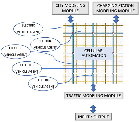
Figure 1.
Application Modules. The city modeling module, the CS modeling module, and the traffic modeling module interact directly with the CA. The EVs are modeled as agents that execute a complex behavior only in those cells in which the EV resides.
2.1.1. City Modeling Module
The city is a synthetic and regular grid composed of a set of cells that form a 2D lattice. Periodic boundary conditions are employed, so its final topology is a 2D torus. Each city cell has a set of properties inspired by the works of Chopard et al. [16,17].
The model of the city consists of different tiles (group of cells) that are joined together, forming different structures. We can create regular city patterns by combining these tiles.
Tile ensembles can be the following:
- Streets: group of cells joined together following the same direction and forming a single lane. There are only four directions: north, east, south and west.
- Avenues: group of cells joined together following the same direction, but forming two lanes. The speed in this type of roads is higher than those of the streets.
- Intersections: structure formed when two streets cross each other.
- Roundabouts: structure formed when two avenues cross each other. It has an internal rotary element of varying radius and multiple entrances and exits.
A visual representation of the 2D lattice base pattern is shown in Figure 2a. As we want to create a microscopic model, each cell has a length of 5 m and we consider that it can only accommodate one vehicle. Each cell in the city has a type that is colored differently so that we can distinguish different structures. This pattern can be scaled or resized to build a portion of a city where long avenues are joined by roundabouts. The area enclosed by avenues can be considered as composed of small streets with shops, housing, offices, etc. A small visualization of this kind of city is depicted in Figure 2b.
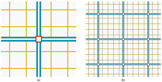
Figure 2.
Synthetic city visualization. Roundabouts are colored in red, avenues are represented in blue, and streets are in pale yellow. Background cells in light gray color are not part of the road system. (a) Base pattern. (b) Small regular city.
2.1.2. Traffic Modeling Module
There are no traffic lights nor traffic signs in the city that control the traffic. Rules are:
- Each city cell has a set of roads that can be reached from its position. Therefore, a vehicle in a certain cell can only take positions for the next step from this cell set. That is, the city is represented as a directed graph.
- Two vehicles cannot overlap in the same position while they are moving. They can only overlap when parked or at a CS.
- The speed is the same for every road in the city except on avenues, where it is double.
- Every city cell can be used as a parking space or as a CS. When the vehicles are parked or in a CS, they are invisible to the rest of the vehicles.
The movement of vehicles is computed using a path-finding algorithm from its current position to its target. The algorithm employed is an A* algorithm with the heuristic of first choosing those cells closest to the target [25]. The movement of vehicles evolves according to a finite state machine consisting of 6 different states:
- a
- Driving towards destination: In this state, vehicles have a destination position, so they try to follow the path proposed by the A* algorithm. If the vehicle cannot move to that position (because it is already occupied by another vehicle), it has a small probability to move to a random position reachable from its current cell. If the battery of an EV drops below a certain threshold, it changes to the state ‘Driving towards station’.
- b
- At destination: The vehicle has reached its destination and it waits there for a certain amount of time, which is modeled as a normal distribution, described in Section 2.1.3. After this waiting time, the vehicle chooses another destination position and changes to state ‘Driving towards destination’.
- c
- Driving towards station: The vehicle has a target station and drives towards it in the same fashion as with a destination. Once it reaches the station, the vehicle changes to ‘At station’ state.
- d
- At station. When the vehicle arrives at the station, it can either start charging right away because there are available chargers, or wait until one charger is available.
- e
- Charging state. The vehicle charges its battery until it reaches its goal level of charge. This goal level is computed following a normal distribution, as described in Section 2.1.3. When the charging is over, the vehicle changes to state ‘Driving towards destination’ and it resumes its journey to its destination.
- f
- Dead-battery state. If for some reason, the vehicle runs out of battery, it will be invisible for the rest of the vehicles. It will not occupy any space and will remain in this state until the end of the simulation.
2.1.3. EV Modeling Module
In normal streets, EVs advance 1 cell if the next cell is free, and they spend 1 energy unit of their batteries for that. In the avenues, they advance 2 cells at each time step, but for this, they spend 2 energy units. That is, we have considered a simple energy model in which energy consumption is proportional to speed. This is consistent with experimental data measured in [26], where an approximately linear relationship between power consumption and speed of an EV was found, for speeds below 50 km/h. When the battery charge of an EV is below one fourth of the total charge, it changes to the ‘Driving towards station’ state (that is, it falls into a seeking mode) and follows a path to the nearest CS. We have used one of the most sold EVs of previous years, 2014 Nissan Leaf, as a reference vehicle for our simulations. The values measured by the U.S. Environmental Protection Agency for this vehicle have been chosen for the total range (autonomy) and for the battery capacity of the EVs in our model: a mean range of 135 km and a 24 kWh battery [27]. When choosing the reference vehicle, we have taken into account that our case study is designed for current urban traffic. The battery capacity of electric cars available on the market today ranges from values around 6 kWh for very small vehicles such as Renault Twizy, to around 100 kWh for high-end models such as Tesla Model S. However, many of the cars circulating in current cities are still models from previous years. In addition, small vehicles (with low battery capacity) are especially popular for driving and parking in large cities. Therefore, we have used a moderate value (24 kWh) for the battery capacity of EVs in our simulation. Bearing in mind that each cell in our model has a length of 5 m (i.e., 200 squares of our grid are equivalent to 1 km), the vehicle autonomy in time steps is given by Equation (1).
We have considered an average speed in streets of 10 km/h and 20 km/h for avenues. This is a rounded figure (for simplicity) which is consistent with data reported by the administration of London of an average speed of km/h for the central London area and km/h for the inner London area (districts surrounding central London), from 10:00 to 16:00, in 2016/2017 [28]. The administration of Paris reported a value of the same order of magnitude for the average speed in the central area, from 7:00 to 21:00, in 2019: km/h [29].
The average real-time equivalent of one time step of our simulations is calculated in Equation (2), bearing in mind that a mean range of 135 km driving at an average speed of 10 km/h (in streets) means a driving time of h.
The initial EV battery charge when the simulation starts and the amount of charge that EVs recharge at stations are modeled by a normal probability distribution (Equation (3)). We have taken for the mean a half the mean range of the reference vehicle, km, and for the standard deviation a fraction of the mean, . Similarly, for the simulation to be realistic, all EVs do not start traveling at the same time at the first time step. Instead, a waiting time is introduced, which is also modeled by a normal probability distribution (Equation (3)) with parameters min and . Once an EV reaches its destination, a similar waiting time is introduced before it starts traveling again to a new destination. Since normal distributions have infinite ranges, we have truncated them so that we only get values within a finite range. The configuration of these parameters following a normal distribution is important to avoid anomalous initial transient periods and to reach stationary behaviors faster (see Section 3.3).
2.1.4. CS Modeling Module
The stations are special road cells that do not occupy space. So, the vehicles inside the station are invisible to the rest of the traffic. We are assuming that the station has an infinite amount of parking space for the vehicles to recharge and to wait for an available charger. We make this assumption since we want to capture the traffic problems caused by the location of the station and the behavior of EVs moving towards them. On the contrary, we are not interested in modeling a row of vehicles lining up outside a station. Our assumptions correspond well with underground CSs.
According to [30], in 2018, most of the direct current (DC) chargers across the European Union offered 50 kW of power. They acknowledged that there is a trend to increase the power of DC stations between 100–150 kW, but a further increase is only beneficial for a limited range of vehicles, at least in the short and medium term. Moreover, they pointed out disadvantages of high-power DC chargers like battery strain. Since we want to study the effects of placing the stations, we are using the de facto industry standard and all the chargers in the stations are supposed to have a power of 50 kW to prevent that charging time lasts several hours. Thus, cars stay in the CSs for around half an hour before resuming their travel.
For this study, we have considered three types of CS arrangements around the synthetic city: one large station with many chargers, four medium sized stations, and a larger number of small stations. In order to make a fair comparison, the total number of chargers (i.e., the sum of the number of chargers of every station) is the same for the three different dispositions.
3. Results and Analysis
First, several preliminary tests were done to check the robustness of our simulator. As the street configuration is synthetic, it was proven that, without EVs that may alter the traffic around CSs, the traffic distribution was similar for different city sizes and for the same conditions.
We performed the tests using a city size sufficiently large enough to be realistic (5 km2 with six avenues), but not too large, so that the number of cells was low enough to execute a 1000-min simulation (sufficient to reach the stationary state of the city traffic) in several minutes.
This allowed us to run ten times a complete set of tests, varying the different parameters in approximately two days on a moderate size server (32 nodes summing a total of 372 cores of architecture Intel x86-64). This size was shown to be adequate to compare and find the better station arrangement for the different parameters (amount of traffic, proportion of EVs, initial EV conditions, etc.).
We have tried three different arrangements of stations, but with the same number of chargers. The three dispositions were defined as follows:
- 1 central station placed on an avenue with 72 chargers.
- 4 evenly distributed stations on avenues having 18 chargers each.
- 36 evenly distributed stations placed on streets (not on avenues) having 2 chargers each.
The number of vehicles in the city is taken as a proportion of the drivable cells in the city:
Besides, the number of EVs in the city is taken as a proportion of the total number of vehicles in the city:
An initial set of simulations was first carried out to find which values of can be considered as low traffic conditions, and which others lead to the first bottlenecks, mainly around the CSs. Approximately, the thresholds were found to be = and a low = . Below these thresholds, traffic conditions were almost ideal (no bottlenecks, mean speed remains constant), thus, these results are of no interest, and they are not shown here.
In order to evaluate the deployment of CSs, we have measured the following metrics for each simulation: the mean intervals that EVs spent at each state (mainly those of queuing in the station and seeking a station), the mean speed of all the vehicles (combustion and electric ones) and the cell occupancy rates that reveal bottlenecks in specific places. Graphs containing mean values are shown with deviation bars for 10 simulations with different random initial conditions.
3.1. EV State Distribution
First, we have analyzed the distribution of states of EVs during the simulation, for the three different CS layouts and different values of the parameters. This first set of tests demonstrates the correct working of our simulator and draws some first interesting results. We analyze the time spent by EVs in their two main stages that distinguish them from a combustion vehicle: (a) the mean time spent while going to the CS, that is, the mean time that a vehicle needs to reach a station once it has detected its requirement to be recharged (denoted as EV seeking time); and, (b) the elapsed time since the vehicle reached the station until a charger was available and it started to recharge (denoted as EV queuing time).
In Figure 3, we present three graphs with the EV seeking time for different values of . Evidently, a low proportion (10%) of EVs means that their effects on the traffic are minimized since 90% of the vehicles are ICEVs and moving around the city without the need to recharge. Obviously, the more vehicles moving in the city, the longer the search times, as a consequence of the higher traffic density. As expected, this occurs smoothly and gradually for the distributed station cases, but a remarkable effect begins to appear for one big central station: there is a threshold in the vehicle density (or in the total number of vehicles), for which seeking times visibly rise. This critical level supposes a total number of 7000 vehicles for 10% of EVs, and decreases progressively with increasing . This is the primary effect pointing to traffic saturation around the big central station, which does not appear when the stations are distributed. What is more, traffic saturation is mitigated somewhat by the assumption that there are infinite waiting places inside the stations, which means that many cars are in fact not contributing to traffic jams.
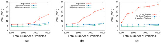
Figure 3.
Mean time spent while going towards the station (seeking time). (a) . (b) . (c) .
It is also logical that standard deviations for the set of tests are high, as the total number of vehicles approaches the threshold, which means that the traffic is problematic and has a high dependence on the chosen (random) initial conditions. This is very visible for the cases of a central station, due to the hot traffic spot found around the single station.
The next remarkable aspect is the mean time that vehicles spend queuing inside stations. Figure 4 contains three graphs, one for each EV density, depicting this EV queuing time for each station arrangement. For , these times are negligible (less than one minute) in all cases. However, we notice for a larger that queues at the stations grow progressively with more vehicles. This effect is significant when multiple small-size stations are tested, due to an unbalanced distribution of EVs and stations; i.e., some stations (which differ according to the initial conditions) suffer from saturation while others are almost empty, leading to an increase in the mean queuing time. For a high EV density (), this problem tends to be intolerable (one hour queuing), indicating that the number of chargers is clearly insufficient when there are more than 5000 vehicles (2500 EVs).
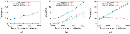
Figure 4.
Mean time spent inside the station without charging (queuing). Notice that the three graphs have different y-axis scales. (a) . (b) . (c) .
Therefore, the weak point of the distributed configuration is the saturation of some specific stations, since the more dispersed the stations are, the more likely it is to occur. It is clear that this problem should be avoided by introducing smart routing into the behavior of EV agents. Vehicles would have information about the occupancy of each station and, perhaps, the traffic conditions, and would choose accordingly. This opens up a miscellaneous set of options in the simulator, which is intended for future work.
3.2. Global Traffic Status and Collapse Conditions
The previous subsection shows that detecting traffic thresholds is crucial to extract interesting conclusions about the arrangement of stations. The main parameter that indicates traffic saturation is the mean speed of vehicles. Figure 5 shows the mean speed for different scenarios and the total number of cars. In general, the speed remains constant (meaning that there are no traffic jams or congestion in the simulations) until a certain threshold is reached. Once again, this is more abrupt for the case of having only one big station: here, EVs congest the surroundings of the station and cause a malfunction of the whole city.
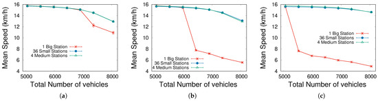
Figure 5.
Average speed across the simulations. (a) . (b) . (c) .
Considering these conditions, we conclude that the critical parameters for the small city presented here are of the drivable cells occupied by vehicles and of EVs. By investigating these values in greater detail, we can draw the main conclusions, which should be predicted by urban designers to prevent these problematic situations. This is analyzed in the next subsection.
3.3. EV State Evolution
Mean values for the whole simulation give a big picture of the traffic and charging behavior, but it does not allow us to identify the reasons for an abnormal situation when approaching the threshold values that begin to collapse the city. Observing the evolution of the vehicle’s states sheds light on the reasons for this situation and its consequences. An interesting case is shown in Figure 6 for the critical parameters , for two different station arrangements. We can distinguish 3 or 4 periods along the complete 1000 min simulation.
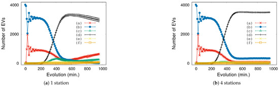
Figure 6.
Each curve represents the number of EVs in a particular state across a simulation with and . (a) Driving towards destination, (b) At destination, (c) Driving towards station, (d) At station, (e) Charging state, (f) Dead-battery state.
The first transient period (from 0 to approximately minute 200) obviously depends on the initial conditions. In this case, the initial state for every car is declared as “At destination” (b), meaning that after some time (defined as a Gaussian distribution), it starts moving towards a new destination, entering the state “Driving towards destination” (a). Note that the other Gaussian distribution for the initial charge assumes that each car has enough energy to start moving.
In the second transient (200-500 min. approximately), the vehicles need to recharge their batteries. Once they arrive at the station, they take available chargers. In some minute, the number of vehicles in “Charging state” (e) reaches its maximum (in our simulations, only 72 chargers are available). This means that the following vehicles entering the station necessarily remain in “At station” state (b) waiting for a free charger (that is, in mode “queuing time”).
At the end of this second transient, we can find two very different behaviors: the case of distributed stations (Figure 6, right) enters a stationary state, but the case of a central station (Figure 6, left) continues its evolution. Evidently, the few chargers of this layout imply that most cars are forming a queue to wait for a free charger. However, and paradoxically, a simple visual inspection seems to indicate that the case of a central station is behaving better than the other one because the number of cars in “At station” state starts to decrease (around minute 700). However, the truth is very different when a detailed examination is carried out: during the second transient (around minute 300) the number of cars going towards a station grows far more for the central station than for the distributed case. The real reason for this difference is that a traffic jam starts to appear around the central station (see Section 3.2 and Figure 5), so it takes a long time for cars to reach the station.
After some minutes (min. 650), this results in the battery of some EVs being drained, clearly indicating that this disposition is not practical. The rest of the curves behave accordingly due to this traffic jam effect: the number of vehicles in “Driving towards destination” and “Driving towards station” states increases steadily and simply, because many vehicles are spending more and more time in the traffic jam; the number of vehicles at a destination tends to zero because they are waiting in the other states.
Finally, note that there is an important dispersion for the different trials in Figure 6 (left) once the traffic jam is reached, because this condition depends on the initial condition and on the specific points at which traffic starts to increase.
This is also supported by the “heat map” of the traffic during the simulation. Figure 7 shows three visual representations of the amount of traffic in the city during three instants for the case of a central station with the same conditions as those of Figure 6. We can observe that the area surrounding the central station (located at the middle cross) is becoming increasingly congested, leading, in the end, to a global deadlock in the city.
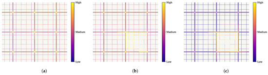
Figure 7.
Amount of traffic in the city throughout the simulation. (a) 1/3 of simulation. (b) 2/3 of simulation. (c) end of simulation.
4. Conclusions and Future Work
In this work, we present a cellular-automata and agent-based hybrid model and a simulation tool implementing this model to analyze the layout of CSs deployment in cities. Our model and tool allow the execution of microscopic traffic simulations, tracing the behavior of individual vehicles, which include EVs, ICEVs and CSs. Each EV is modeled as an agent incorporating a complex behavior which involves decisions about the following factors: the specific destination of each vehicle, the route to follow, how to navigate there, taking into account the local traffic state, when to drive to a CS to recharge the battery, and what station to drive to.
Our study has been useful to analyze the effects of different dispositions of CSs in a city. We have found very different consequences for a large central station versus a set of smaller distributed stations.
In the case of a single central station, we found that when the vehicle density exceeds a certain critical level, a large traffic jam is formed in a wide area around the central station. It collapses the city and causes an abrupt decrease in the mean speed of vehicles, even resulting in many EVs running out of battery. We also verified the effects of this collapse directly in the ‘heat map’ of the amount of traffic, in the evolution of the number of EVs at each state and in the high increase of the time spent by EVs driving towards a CS.
This situation does not happen for the distributed CS layout: here, the city reaches a stationary state in which the traffic is fluid. However, we also found that a distributed layout conveys the following drawback: the time spent by EVs queuing in the CS (that is, waiting for a free charger) gets higher than for a single large station when the vehicle density increases. The reason is an unbalanced distribution of EVs among the different CSs, so that some of them become saturated, while other ones still hold free chargers.
Our results are useful for urban designers, planners and policy makers. First, our study shows that the best arrangement of public CSs in a city is a distributed network, which avoids the serious traffic jam introduced by a single central station, which indeed affects severely the traffic conditions in the whole city. Second, it is very important to introduce smart routing measures to balance the distribution of EVs among the different CSs in the distributed network. These measures can range from placing information signs showing the occupancy level of each CS to implementing an intelligent traffic management system that directly interacts with the EVs or with their users.
The work presented here is a first step that opens up very promising perspectives for further research directions, which we plan to undertake in the future.
Firstly, our simulator can be used to investigate other ‘what if’ scenarios, involving, for example, other patterns in the CS layout, how the location of traffic attraction areas (e.g., large shopping malls) affects the CS network and traffic, or how specific massive events (such as large sport competitions) or emergency situations can affect the charging network and the traffic.
Secondly, the results presented in this work indicate that an extension of our tool to incorporate geographic data from a real city extracted using a geographic information system (GIS) is of great interest. This extended tool can be highly valuable for predicting the effects of the layout of the CS network on urban traffic in real cities and for studying the optimal deployment of these stations. To carry out such a study of a real city, it will be important to take also into account a lot of city peculiarities as additional inputs, such as the urban planning policy, the land use, the power grid and so on.
Thirdly, this model and tool can also be extended to build a traffic simulation framework to study the effects of intelligent traffic management algorithms on EV traffic and CS network. To this end, the agents of our model should be provided with inputs coming from a smart city traffic management system, including information such as the current occupancy level of each CS, the current traffic state in each part of the city, or even predictions of intelligent algorithms about the near future states. Our tool is thus a first step towards an intelligent traffic management simulation system for both electric and combustion vehicles and for CSs in smart cities.
Author Contributions
Conceptualization, A.G.-S., J.-L.G.-L., F.D.-d.-R. and F.J.-M.; methodology, A.G.-S., J.-L.G.-L., F.D.-d.-R. and F.J.-M.; software, A.G.-S.; validation, A.G.-S., J.-L.G.-L., F.D.-d.-R. and F.J.-M.; formal analysis, A.G.-S., J.-L.G.-L., F.D.-d.-R. and F.J.-M.; investigation, A.G.-S., J.-L.G.-L., F.D.-d.-R. and F.J.-M.; resources, A.G.-S., J.-L.G.-L., F.D.-d.-R. and F.J.-M.; data curation, A.G.-S.; writing–original draft preparation, A.G.-S., J.-L.G.-L., F.D.-d.-R. and F.J.-M.; writing–review and editing, A.G.-S., J.-L.G.-L., F.D.-d.-R. and F.J.-M.; visualization, A.G.-S.; supervision, J.-L.G.-L. and F.D.-d.-R. and F.J.-M.; project administration, J.-L.G.-L.; funding acquisition, J.-L.G.-L., F.D.-d.-R. and F.J.-M. All authors have read and agreed to the published version of the manuscript.
Funding
This research was funded by Ministerio de Ciencia e Innovación - Agencia Estatal de Investigación of Spain, cofinanced by FEDER funds (EU), project MABICAP (Bio-inspired machines on High Performance Computing platforms: a multidisciplinary approach, TIN2017-89842P) and project Par-HoT (PID2019-110455GB-I00).
Institutional Review Board Statement
Not applicable.
Informed Consent Statement
Not applicable.
Acknowledgments
We want to thank the Centro Informático Científico de Andalucía (CICA) for providing the high performance computing cluster, in which we performed the simulations. We would also like to thank the anonymous reviewers and the editors of this journal for their detailed and helpful comments, which helped improve and clarify this manuscript.
Conflicts of Interest
The authors declare no conflict of interest. The funders had no role in the design of the study; in the collection, analyzes, or interpretation of data; in the writing of the manuscript, or in the decision to publish the results.
Abbreviations
The following abbreviations are used in this manuscript:
| EV | electric vehicle |
| ICEV | internal combustion engine vehicle |
| CS | charging station |
| CA | cellular automata |
| ABM | agent-based model |
| DC | direct current |
References
- EY Mobility Center. Guía de Movilidad eléctrica Para Entidades Locales (Electric Mobility Guide For Local Entities); Technical Report; Red Eléctrica de España (REE): Alcobendas, Spain; Federación Española de Municipios y Provincias (FEMP): Madrid, Spain; Instituto para la Diversificación y Ahorro de la Energía (IDAE): Madrid, Spain, 2019. [Google Scholar]
- Cieslik, W.; Szwajca, F.; Golimowski, W.; Berger, A. Experimental Analysis of Residential Photovoltaic (PV) and Electric Vehicle (EV) Systems in Terms of Annual Energy Utilization. Energies 2021, 14, 1085. [Google Scholar] [CrossRef]
- Zhang, J.; Wang, Z.; Liu, P.; Zhang, Z. Energy consumption analysis and prediction of electric vehicles based on real-world driving data. Appl. Energy 2020, 275, 115408. [Google Scholar] [CrossRef]
- Chłopek, Z.; Lasocki, J.; Wójcik, P.; Badyda, A.J. Experimental investigation and comparison of energy consumption of electric and conventional vehicles due to the driving pattern. Int. J. Green Energy 2018, 15, 773–779. [Google Scholar] [CrossRef]
- Li, Y.; Luo, J.; Chow, C.Y.; Chan, K.L.; Ding, Y.; Zhang, F. Growing the charging station network for electric vehicles with trajectory data analytics. In Proceedings of the 2015 IEEE 31st International Conference on Data Engineering, Seoul, Korea, 13–17 April 2015; pp. 1376–1387. [Google Scholar] [CrossRef]
- Dong, J.; Liu, C.; Lin, Z. Charging infrastructure planning for promoting battery electric vehicles: An activity-based approach using multiday travel data. Transp. Res. Part C Emerg. Technol. 2014, 38, 44–55. [Google Scholar] [CrossRef]
- Liu, Q.; Liu, J.; Le, W.; Guo, Z.; He, Z. Data-driven intelligent location of public charging stations for electric vehicles. J. Clean. Prod. 2019, 232, 531–541. [Google Scholar] [CrossRef]
- Guo, C.; Yang, J.; Yang, L. Planning of Electric Vehicle Charging Infrastructure for Urban Areas with Tight Land Supply. Energies 2018, 11, 2314. [Google Scholar] [CrossRef]
- Gao, H.; Liu, K.; Peng, X.; Li, C. Optimal Location of Fast Charging Stations for Mixed Traffic of Electric Vehicles and Gasoline Vehicles Subject to Elastic Demands. Energies 2020, 13, 1964. [Google Scholar] [CrossRef]
- Xu, M.; Meng, Q. Optimal deployment of charging stations considering path deviation and nonlinear elastic demand. Transp. Res. Part B Methodol. 2020, 135, 120–142. [Google Scholar] [CrossRef]
- Kong, W.; Luo, Y.; Feng, G.; Li, K.; Peng, H. Optimal location planning method of fast charging station for electric vehicles considering operators, drivers, vehicles, traffic flow and power grid. Energy 2019, 186, 115826. [Google Scholar] [CrossRef]
- Pruckner, M.; German, R.; Eckhoff, D. Spatial and temporal charging infrastructure planning using discrete event simulation. In Proceedings of the SIGSIM-PADS 2017—Proceedings of the 2017 ACM SIGSIM Conference on Principles of Advanced Discrete Simulation, Singapore, 24–26 May 2017; Association for Computing Machinery, Inc.: New York, NY, USA, 2017; pp. 249–257. [Google Scholar] [CrossRef]
- Islam, M.M.; Shareef, H.; Mohamed, A. Improved approach for electric vehicle rapid charging station placement and sizing using Google maps and binary lightning search algorithm. PLoS ONE 2017, 12, e0189170. [Google Scholar] [CrossRef]
- Deb, S.; Gao, X.Z.; Tammi, K.; Kalita, K.; Mahanta, P. A novel chicken swarm and teaching learning based algorithm for electric vehicle charging station placement problem. Energy 2021, 220, 119645. [Google Scholar] [CrossRef]
- Nagel, K.; Schreckenberg, M. A cellular automaton model for freeway traffic. J. Phys. I 1992, 2, 2221–2229. [Google Scholar] [CrossRef]
- Chopard, B.; Luthi, P.O.; Queloz, P.A. Cellular automata model of car traffic in a two-dimensional street network. J. Phys. A Math. Gen. 1996, 29, 2325–2336. [Google Scholar] [CrossRef]
- Dupuis, A.; Chopard, B. Parallel simulation of traffic in Geneva using cellular automata. In Virtual Shared Memory for Distributed Architectures; Kühn, E., Ed.; Nova Science: Commack, NY, USA, 2001; pp. 89–107. [Google Scholar]
- Li, X.G.; Jia, B.; Gao, Z.Y.; Jiang, R. A realistic two-lane cellular automata traffic model considering aggressive lane-changing behavior of fast vehicle. Phys. A Stat. Mech. Appl. 2006, 367, 479–486. [Google Scholar] [CrossRef]
- Zheng, Y.L.; Zhai, R.P.; Ma, S.Q. Survey of cellular automata model of traffic flow. J. Highway Transp. Res. Dev. 2006, 23, 110–115. [Google Scholar]
- Xiang, Y.; Liu, Z.; Liu, J.; Liu, Y.; Gu, C. Integrated traffic-power simulation framework for electric vehicle charging stations based on cellular automaton. J. Mod. Power Syst. Clean Energy 2018, 6, 816–820. [Google Scholar] [CrossRef]
- Chen, B.; Cheng, H.H. A review of the applications of agent technology in traffic and transportation systems. IEEE Trans. Intell. Transp. Syst. 2010, 11, 485–497. [Google Scholar] [CrossRef]
- Waraich, R.A.; Galus, M.D.; Dobler, C.; Balmer, M.; Andersson, G.; Axhausen, K.W. Plug-in hybrid electric vehicles and smart grids: Investigations based on a microsimulation. Transp. Res. Part C Emerg. Technol. 2013, 28, 74–86. [Google Scholar] [CrossRef]
- Viswanathan, V.; Zehe, D.; Ivanchev, J.; Pelzer, D.; Knoll, A.; Aydt, H. Simulation-assisted exploration of charging infrastructure requirements for electric vehicles in urban environments. J. Comput. Sci. 2016, 12, 1–10. [Google Scholar] [CrossRef]
- Zhai, Z.; Su, S.; Liu, R.; Yang, C.; Liu, C. Agent–cellular automata model for the dynamic fluctuation of EV traffic and charging demands based on machine learning algorithm. Neural Comput. Appl. 2019, 31, 4639–4652. [Google Scholar] [CrossRef]
- Hart, P.E.; Nilsson, N.J.; Raphael, B. A Formal Basis for the Heuristic Determination of Minimum Cost Paths. IEEE Trans. Syst. Sci. Cybernet. 1968, 4, 100–107. [Google Scholar] [CrossRef]
- Wu, X.; Freese, D.; Cabrera, A.; Kitch, W.A. Electric vehicles’ energy consumption measurement and estimation. Transp. Res. Part D Transp. Environ. 2015, 34, 52–67. [Google Scholar] [CrossRef]
- EPA. Fuel Economy Guide; Technical Report; U.S. Environmental Protection Agency (EPA): Laurel, MD, USA, 2014.
- Transport for London. Travel in London Report 10; Technical Report; Transport for London, Mayor of London: London, UK, 2017.
- Direction de la Voirie et de Déplacements. Le Bilan Déplacements en 2019 à Paris; Technical Report; Direction de la Voirie et de Déplacements, Mairie de Paris: Paris, France, 2019.
- Spöttle, M.; Jörling, K.; Schimmel, M.; Staats, M.; Grizzel, L.; Jerram, L.; Drier, W.; Gartner, J. Research for TRAN Committee—Charging Infrastructure for Electric Road Vehicles; Technical Report; Policy Department for Structural and Cohesion Policies, European Parliament: Brussels, Belgium, 2018.


Publisher’s Note: MDPI stays neutral with regard to jurisdictional claims in published maps and institutional affiliations. |
© 2021 by the authors. Licensee MDPI, Basel, Switzerland. This article is an open access article distributed under the terms and conditions of the Creative Commons Attribution (CC BY) license (https://creativecommons.org/licenses/by/4.0/).