An Integrated Bus Holding and Speed Adjusting Strategy Considering Passenger’s Waiting Time Perceptions

Abstract

To solve the problems of bus bunching and large gaps, this study combines bus holding and speed adjusting to alleviate them respectively considering the characteristics of passenger’s perceived waiting time. The difference between passenger’s perceived waiting time at stops and actual time is described quantitatively through the expected waiting time of passengers. Bus holding based on a threshold method is implemented at any stops for bunching buses, and speed adjusting based on a Markovian decision model is implemented at limited stops for lagging buses. Simulations based on real data of a bus route show that the integrated control strategy is able to improve the service reliability and to decrease passengers’ perceived waiting time at stops. Several insights have been uncovered through performance analysis: (1) The increase of holding control strength results in improvement of the headway regularity, and leads to a greater perceived waiting time though; (2) Compared to traveling freely, suitable speed guidance will not slow down the average cruising speed in the trip; (3) The scale of passenger demand and through passengers are the two key factors influencing whether a stop should be selected as a speed-adjusting control point.

1. Introduction

Bus bunching and large gaps commonly happen on high-frequency bus routes [1], and lead to an unreliable service; these usually appear in tandem. Their occurrence is mainly affected by two uncertain factors: the disturbance by private cars of the bus journey and variation of the passenger demand to be served. Due to these factors, bus bunching and large gaps tend to worsen if measures are not taken to alleviate them, and will cause serious instability at the level of the overall bus system [2].

On the one hand, the occurrence of bus bunching and large gaps leads to irregularity of the headway, which means longer waiting times and lower passenger satisfaction at stops. On the other hand, the capacities of buses in the fleet are quite unbalanced [1]. Some buses are overcrowded with passengers, while others carry only a few, which means inefficient utilization of the bus capacity and an uncomfortable service for passengers in vehicles (riders). Thus, reducing bus bunching and large gaps is beneficial to both passengers and the transit agency.

Many researchers have proposed effective control methods, including bus holding and speed adjusting. Nowadays, with the development of intelligent transit technologies, more meticulous integrated strategies with two or more control methods have been in the focus of more and more researchers. At the same time, greater emphasis is placed on bus users’ satisfaction and control strategies involving passenger perceptions. Public transit is a more energy-efficient and environmentally friendly travel mode than driving private vehicles. Taking into account the passenger’s perceived waiting time can make operation control more realistically consider the passenger’s travel experience, which is conducive to improving the attractiveness of public transit to passengers and the sustainable development of urban traffic. This study shows an integrated bus holding and speed adjusting strategy considering passenger perceptions to reduce bus bunching and large gaps and improve both the reliability of the transit service and passenger satisfaction. The remainder of this paper is organized as follows: Chapter 2 reviews the recent literature on the themes of bus holding control, speed adjusting, and transit passenger perceptions. Chapter 3 models the passengers’ perceived waiting time at the stop. Chapter 4 presents the integrated control strategies to reduce bus bunching and large gaps. Chapter 5 analyzes the performance at different locations where speed adjusting can be executed and the effectiveness of the integrated control strategy to improve passenger perceptions. Chapter 6 presents some concluding insights.

2. Literature Review

2.1. Bus Holding Control

Many studies demonstrate that holding is an effective method to reduce bus bunching. This refers to detaining a bus for an extra time after allowing all the passengers to board and alight, so as to enlarge the headway between the bus being held and the preceding bus (i.e., forward headway) to prevent bus bunching. Because restoration of the forward headway to stability enables the current bus to relieve the imminent passenger demand at the stops for the following bus, both bus bunching and large gaps can be alleviated to some extent through holding control.

Some holding control models include the notion of a pre-specified headway or pre-specified timetable. Pre-specified headways are often related with the dispatching interval. Daganzo [2] proposed a headway-based adaptive control and Xuan et al. [3] extended Daganzo’s research to schedule reliability. Fu et al. [4], Cats et al. [5], Yin et al. [6], and Huang et al. [7] all considered the threshold headway to activate holding control. Chen et al. [8] and Alesiani et al. [9] established a reinforcement learning model for holding control. These models involving pre-specified headway have intuitive and interpretable parameters of headway, by means of which the service reliability and in-vehicle delays can be adjusted in the desired direction.

Some researchers put forward a series of self-equalizing holding control methods, which disregard the pre-specified headway and make the headway of the bus fleet gradually converge to a natural value. Bartholdi et al. [10] developed a self-coordination holding method based on a Markov chain model. Liang et al. [11] proposed a two-way-looking self-equalizing control method, including the concept of the convergence rate. Zhang et al. [12] discussed the convergence properties of two-way-looking holding control under deterministic and stochastic traveling time and parameter optimization. The headways in the above methods tend to converge, even with only one control point. Simplifying the job of the drivers enables them to concentrate more on driving itself.

Moreover, some studies either involved a pre-specified headway or have a tendency to convergence of the headway. These control models were established with the variables of the waiting times at the stop and in-vehicle delays immediately. Delgado et al. [13] studied an integrated bus holding and limited boarding strategy within a rolling horizon framework. Sánchez-Martínez et al. [14] extended the work of Delgado. They proposed that holding control that reflects dynamic running times and demand elicits lower passenger costs. Berrebi et al. [15] compared holding control strategies with and without real-time prediction. Chen et al. [16] proposed an integrated bus holding and limited boarding strategy, which predicts the perceived waiting times at several downstream stops, while deciding the holding times/number of passengers to be denied boarding at the current stop. Wang et al. [17] extended the work of Chen et al. [8] and Alesiani et al. [9] without a pre-specified headway. The above studies implemented control strategies with variable headways.

2.2. Speed Adjusting Control

When the current bus is suffering from bunching and its backward headway is rising beyond a certain critical value, holding control of the current bus cannot alleviate the load of the following bus effectively due to the increasing demand. The following bus is therefore left behind. Thus, many studies introduced the speed adjusting control, which gives guidance on the cruising speed in order to shorten large gaps.

Many researchers proposed speed adjusting methods to be executed at all general road segments. Daganzo et al. [18] developed a control method that dynamically coordinates the speeds of successive cruising buses. Teng et al. [19] used historical data of the cruising speed in corresponding links and obtained dynamic threshold values of headway deviation. Yan et al. [20] aimed at minimizing the average absolute deviation of headway and discussed the methods under the different circumstances of no control, expected control, and control considering the mean speed of the traffic flow. He [21] proposed an integrated bus holding and speed adjusting strategy and, in this study, speed adjusting control is implemented in all general rather than parts of road segments, which may be impeded by the surrounding traffic.

One of the challenges of speed adjusting in practice, that of whether the desired speed can be gained through real-time guidance or not, is mainly influenced by the surrounding traffic. Therefore, a speed adjusting method that is only implemented in dedicated bus lanes (DBL) has attracted researchers’ attention. He et al. [22] overcame the difficulty of implementation mentioned in Daganzo’s study [18]. They proposed a multi-CTP method to improve the operational stability of a bus line containing DBLs. Bie et al. [23] developed an integrated strategy of speed guidance in the bus line and intersection signal control. The buses left behind will pass through and buses too close to the preceding one will be impeded at the intersection, which is very different from bus signal priority.

2.3. Transit Passenger Perceptions

From psychology and ethology, waiting time can be described as either objective or subjective [24]. The objective waiting time is the time period recorded by a chronometer, i.e., the actual waiting time. The subjective waiting time is influenced by a person’s internal/external factors, such as individual habits, experiences, and the platform environment. It is also known as perceived waiting time. Trompet et al. [25] pointed out that excess waiting time is the best option when considering the passenger experience of service regularity. Lv et al. [26] proposed that when the waiting times exceed an expected value, passengers may feel anxious and perceive the waiting times as longer than the actual waiting times, which is detrimental to the attractiveness of the transit service. Teng et al. Authors in [27] formulated passenger perceptions of prolonged waiting/in-vehicle time quantitatively using the passenger density on the platform/in the carriage. Fan et al. [24] employed regression analysis to describe the perceived waiting time as a function of the actual waiting time, stop amenities, weather, time of day, personal demographics, and trip characteristics. Mishalani et al. [28] quantified the relationship between perceived and actual waiting time along with socioeconomic characteristics. Herbon et al. [29] considered the passengers leaving stops due to long waiting times when they determined the optimal dispatching frequency. From these various internal/external factors, it can be concluded that the perceived waiting times are usually longer than the actual times. Internal factors include gender, job, and age while external factors include basic amenities, weather, actual waiting time, passenger density, and so on.

2.4. Summary

The existing studies usually employ bus holding, speed adjusting, or their integration to reduce bus bunching and large gaps. Most of them calculate the overall passenger costs by adding in-vehicle delay to the revised waiting time, which is the simple multiplication of the actual waiting time and a disutility parameter (usually equal to 2). Passenger anxiety arising from long waiting times, which causes the difference of the perceived and actual waiting time, is neglected. Recent studies focusing on the speed adjusting method in bus lanes contribute, to some extent, to the realization in practice. However, they do not discuss where to set the speed control point in terms of the passenger demand profile. Studies about passenger perceptions emphasize analyzing how various factors affect passenger satisfaction, and their models are not suitable for real-time computation of the perceived waiting time in operation control.

Thus, this study makes two main contributions. First, we establish a model of passenger’s perceived waiting time. Passengers’ aversion to long-time waiting at stops is described by the number of passengers waiting at the stop, the current headway, and the expected wait. As we will see in Chapter 3, a general method to calculate perceived waiting times under complete/incomplete service is presented. Second, a Markovian decision model is established for speed adjusting and combined with threshold-based holding control. After estimating the probability transition matrix of the integrated strategy, the operational performance of speed adjusting at different locations can be compared. As a result, we obtain the key factors to consider when selecting the location of speed adjusting, through passengers and the demand at downstream stops. The main notation used throughout the paper is listed in

Table 1. Main notation in this paper.

Notation	Explanation	Notation	Explanation
$W_{i,j}$	Total waiting time of passengers boarding bus $i$ at stop $j$. (s)	$X$	Speed adjusting action set.
${\lambda }_j$	Passenger arrival rate at stop $j$. (pax/min)	$x$	Elements in $X$. (s)
$b_1$	Parameter of waiting expectation.	$x^{*}$	Policy with maximal reward expectation. (s)
$b_2$	Parameter of perceived waiting time.	$f_x$	Reward expectation function.
$H$	Dispatching interval. (min)	$\overrightarrow{S}$	Probability distribution vector.
$h_{i,j}$	Preceding headway of bus $i$ at stop $j$. (min)	$P_x^{j^{*}}$	Probability transition matrix.
$a_{i,j}$	Arrival time of bus $i$ at stop $j$. (min)	$N$	Number of simulation days.
$c_{i,j}$	Holding control time of bus $i$ at stop $j.$ (s)	$t_j$	Link travel time from stop $j$ to $j+1$. (s)
$c_{i,j^{*}}$	Speed-up control time at stop $j^{*}$. (s)	$p_j^{alight}$	Alighting rate at stop $j$.
${\alpha }_1$	Parameter of holding control strength.	$t^{board}$	Boarding time per passenger. (s)
${\alpha }_2$	Slack time. (s)	$t^{alight}$	Alighting time per passenger. (s)
$j^{*}$	Stop index of SCP (speed-up control point).	$B_{i,j}$	Number of passengers boarding bus $i$ at stop $j$. (pax)
$s_{i,j^{*}}$	State value of bus $i$ at stop $j^{*}$.	$B$	Number of boarding passengers affected by operation control in a day. (pax)
${\widehat{s}}_{i,j^{*}}$	Median of state in which $s_{i,j^{*}}$ is.	$O_{i,j}^d$	Load of bus $i$ leaving stop $j$. (pax)
$f_v$	Utility function.	$O^d$	Number of riders affected by operation control in a day. (pax)
$N_s$	Number of discrete states.	$W_s$	Weighted waiting time at stops. (s)
${\delta }_s$	State step. (s)	$W_v$	Weighted in-vehicle delay. (s)
$R$	Reward matrix.	$W$	Total travel cost. (s)

Explanatory notes: Any notation with superscript of $\ast$ or $j^{*}$ is employed at the stops allowing for speed-up control.

, unless otherwise specified.

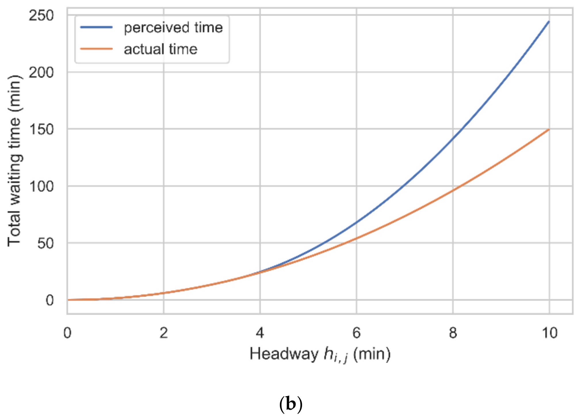
3. Modeling of Passenger’s Perceived Waiting Time

When facing long waiting times, passengers at a stop may feel anxious, perceive their waiting times as longer than they actually are, and then tend to choose other means of transportation. To describe this mental nervousness more exactly, we propose a passenger perceptions model based on the waiting expectation and use this model to calculate the perceived waiting times at the stop. This model involves the following assumptions: (1) Passengers of a high-frequency route arrive at the stop randomly rather than consulting the timetable [5]; (2) Passengers are aware of the dispatching interval $H$, and they expect their waiting times to be no longer than $b_{1}H$, which we call the waiting expectation—$b_1$ is a positive parameter and signifies the ratio of waiting expectation and $H$; (3) The passengers’ perceived waiting time is the piecewise linear function of the actual waiting time; (4) The capacity of a bus is unlimited (if the planning and design of the transit system are well done, this assumption is reasonable [3]). In Appendix A, we derive the model considering the capacity constraints and the passengers denied boarding, conforming to these assumptions, except No. 3.

When the forward headway $h_{i,j}$ of bus $i$ arriving at stop $j$ is less than the waiting expectation $b_{1}H$, i.e., $h_{i,j}=a_{i,j}-a_{i-1,j}<b_{1}H$, all the passengers about to board bus $i$ wait for no longer than $b_{1}H$. Let $w$ be the deviation between the time of the passenger arriving at stop and the last bus $i-1$ arriving at the stop, and $a_{i-1,j}$ be the benchmark. Thus, $w\in \left(0,h_{i,j}\right]$. Passengers who arrive at $w$ wait for $h_{i,j}-w$ seconds. The passenger arrival rate at the stop $j$ is ${\lambda }_j$. The total waiting time $W_{i,j}$ of bus $i$ and stop $j$ is:

$$W_{i,j}={{\displaystyle \int }}_0^{h_{i,j}}{\lambda }_j\left(h_{i,j}-w\right)dw=\frac{{\lambda }_j}{2}{h}_{i,j}^2$$

(1)

When $b_{1}H\le h_{i,j}<2b_{1}H$, the total waiting time can be divided into two parts: 1. Passengers arriving at $\left(h_{i,j}-b_{1}H,h_{i,j}\right]$ wait for less than $b_{1}H$; 2. Passengers arriving at $\left(0,h_{i,j}-b_{1}H\right]$ wait for at least $b_{1}H$ and the earlier they arrive, the longer time they have to wait. Passengers who arrive at $w\in \left(0,h_{i,j}-b_{1}H\right]$ have an excess waiting time of $h_{i,j}-w-b_{1}H$. Excess waiting time refers to the deviation between the actual waiting time and the waiting expectation. The total waiting time $W_{i,j}$ of bus $i$ at stop $j$ is:

$$W_{i,j}=\frac{{\lambda }_j}{2}{h}_{i,j}^2+b_2{{\displaystyle \int }}_0^{h_{i,j}-b_{1}H}{\lambda }_j\left(h_{i,j}-w-b_{1}H\right)dw=\frac{{\lambda }_j}{2}\left[h_{i,j}^2+b_2{\left(h_{i,j}-b_{1}H\right)}^2\right]$$

(2)

where $b_2$ is the parameter denoting that, when a passenger waits for longer than $b_{1}H$, he may feel $\left(1+b_2\right)\times 1$ s passing, while actually only 1 s has passed.

When $n{b}_{1}H\le h_{i,j}<\left(n+1\right)b_{1}H, n=2,3,\dots$, the total waiting time $W_{i,j}$ can be divided into three parts. The total actual waiting time $W_{i,j}^1$ is:

$$W_{i,j}^1=\frac{{\lambda }_j}{2}{h}_{i,j}^2$$

(3)

Some of the passengers arriving at $\left(\left(n-1\right)b_{1}H,n{b}_{1}H\right]$ wait for at least $b_{1}H$, and their arrival time $w\in \left(\left(n-1\right)b_{1}H,h_{i,j}-b_{1}H\right]$. The total excess perceived waiting time $W_{i,j}^2$ of these passengers is:

$$W_{i,j}^2=b_2{{\displaystyle \int }}_{\left(n-1\right)b_{1}H}^{h_{i,j}-b_{1}H}{\lambda }_j\left(h_{i,j}-w-b_{1}H\right)dw$$

(4)

All passengers arriving at $\left(0,\left(n-1\right)b_{1}H\right]$ wait for longer than $b_{1}H$. For passengers arriving at $\left(\left(k-1\right)b_{1}H,k{b}_{1}H\right]$, $k=1,2,\cdots ,n-1$, the total excess perceived waiting time $W_{i,j}^3$ is:

$$W_{i,j}^3=b_2\left[\left(n-1\right){{\displaystyle \int }}_0^{b_{1}H}{\lambda }_j\left(b_{1}H-w\right)dw+{\lambda }_j{b}_{1}H{\displaystyle \sum }_{k=1}^{n-1}\left[h_{i,j}-\left(k+1\right)b_{1}H\right]\right]$$

(5)

The total waiting time $W_{i,j}$ of bus $i$ and stop $j$ is:

$$W_{i,j}=W_{i,j}^1+W_{i,j}^2+W_{i,j}^3=\frac{{\lambda }_j}{2}\left[h_{i,j}^2+b_2{\left(h_{i,j}-b_{1}H\right)}^2\right]$$

(6)

In summary,

$$W_{i,j}=\left\{\begin{array}{c}\frac{{\lambda }_j}{2}{h}_{i,j}^2,if h_{i,j}<b_{1}H\\ \frac{{\lambda }_j}{2}\left[h_{i,j}^2+b_2{\left(h_{i,j}-b_{1}H\right)}^2\right],if h_{i,j}\ge b_{1}H\end{array}\right.$$

(7)

Formula (7) is derived from a complete service, i.e., no passenger will be denied boarding. In fact, we can also model the passengers’ perceived waiting time similarly from an incomplete service, as seen in the Appendix A. From formula (7), we know the following: 1. With a constant ${\lambda }_j$, the larger the headway $h_{i,j}$ is, the more likely passengers are to perceive their waiting time as longer than the actual time; 2. The difference between the perceived waiting time and the actual time, $W_{i,j}-\frac{{\lambda }_j}{2}{h}_{i,j}^2$, is larger than with a relatively smaller ${\lambda }_j$, when passengers are experiencing a large gap. From the perspective of operation control, reducing the excess perceived waiting time should alleviate the emergence of a large gap, while improving the service reliability for as many passengers at as many stops as possible.

Research by Fan et al. [24] shows that stops and stations with high amenities reduce the perceived waiting time to some extent. Thus, we can use parameters $b_{1,j}$, $b_{2,j}$ instead of $b_1$, $b_2$ to represent the differences of amenities, the waiting expectation of various kinds of people, and other factors in the real world. Figure 1a shows the linear relationship between the perceived waiting time and actual waiting time for an individual passenger. Figure 1b shows the relationship between the total waiting time $W_{i,j}$ and the headway $h_{i,j}$.

It should be noted that we are modeling passenger’s waiting time perceptions by involving the notion of a pre-specified headway, i.e., $H$. From formula (7) and Figure 1, we conclude that a large gap is the immediate cause of the increase of the perceived waiting time. In Chapter 4, we will also introduce the operation control method with pre-specified headway to reduce passengers’ perceived waiting time, rather than self-equalizing and the method with variable headway described in subchapter 2.1.

4. Integrated Control Strategy

4.1. Bus Holding

We used the threshold-based holding control to calculate the holding time for buses [4], as seen from formulas (8), (9), and (10). If $h_{i,j}<{\alpha }_{1}H$, bus $i$ will be held for $c_{i,j}=H-h_{i,j}$. ${\alpha }_1$ is the parameter of control strength, ${\alpha }_1\in \left[0,1\right]$, and greater strength means more frequent holdings. $f_{{\alpha }_2}\left(j\right)$ is the function of the stop index and slack time, and ${\alpha }_2$ is the default holding time. Embedding slack time into the holding control results in more resilient operation but more in-vehicle delay. The rules for setting ${\alpha }_2$ are presented in Chapter 5. No slack time is embedded into stop $j^{*}$ and we call stop $j^{*}$ a speed-up control point (SCP), from which the cruising speed of buses leaving can be adjusted. Holding control results in a lower cruising speed; but, in this study, the speed adjusting model is only utilized to speed up cruising in this study.

$$h_{i,j}=a_{i,j}-a_{i-1,j}$$

(8)

$$c_{i,j}=\left\{\begin{array}{c}H-h_{i,j}+f_{{\alpha }_2}\left(j\right), if h_{i,j}<{\alpha }_{1}H\\ \max \left(H-h_{i,j}+f_{{\alpha }_2}\left(j\right),0\right), if h_{i,j}>H\\ f_{{\alpha }_2}\left(j\right), else, 0<{\alpha }_1\le 1\end{array}\right.$$

(9)

$$f_{{\alpha }_2}\left(j\right)=\left\{\begin{array}{c}{\alpha }_2, j\ne j^{*}\\ 0, else\end{array}\right.,{\alpha }_2\ge 0$$

(10)

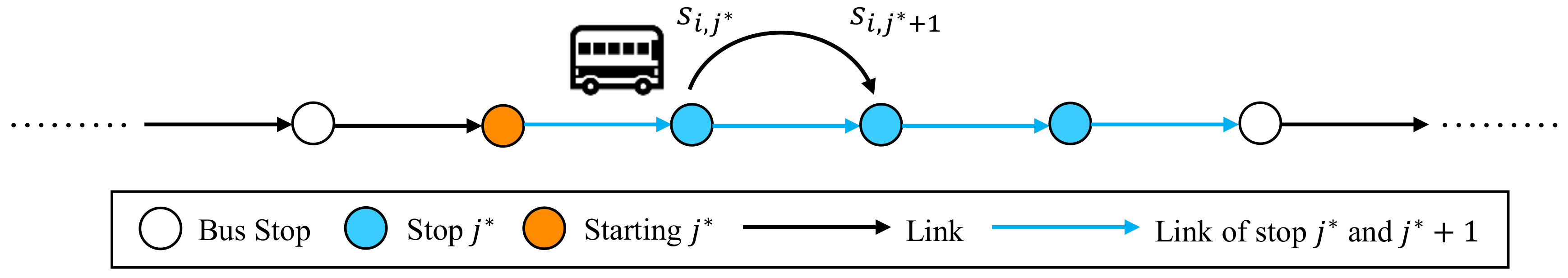
4.2. Speed Adjusting

Based on the assumption of modeling without after-effect, we establish a Markovian decision model $\left(S,X,P,R\right)$ for speed adjusting. When bus 𝑖 leaves from the SCP and is left behind by preceding bus ($h_{i,j}>H$) meanwhile, speed adjusting control within the speed limit may be implemented. $X$ is the control action set and buses left behind are expected to have link travel time $t_{j^{*}}+x, x\in X$. In this study, 4 SCPs are continuously distributed to adjacent bus stops. The discrete stop evolution of bus $i$ traveling from stop $j^{*}$ to $j^{*}+1$ is considered as the time evolution of a stochastic process [30], as shown in Figure 2. This model without after-effect is reasonable for bus operation—a bus leaving early may serve fewer (more) passengers downstream and this phenomenon tends to be enlarged, which finally turns into a bus bunching problem (large gap).

4.2.1. State Definition

When $h_{i,j^{*}}>H$, the state value $s_{i,j^{*}}$ is calculated as follows:

$$s_{i,j^{*}}=a_{i,j^{*}}-a_{i-1,j^{*}}-H=h_{i,j^{*}}-H$$

(11)

where $s_{i,j^{*}}$ is the deviation between the forward headway $h_{i,j^{*}}$ and the dispatching interval $H$, $s_{i,j^{*}}\in \left(-H,+\infty \right]$. When $s_{i,j^{*}}$ is around zero, bus $i$ operates stably in general.

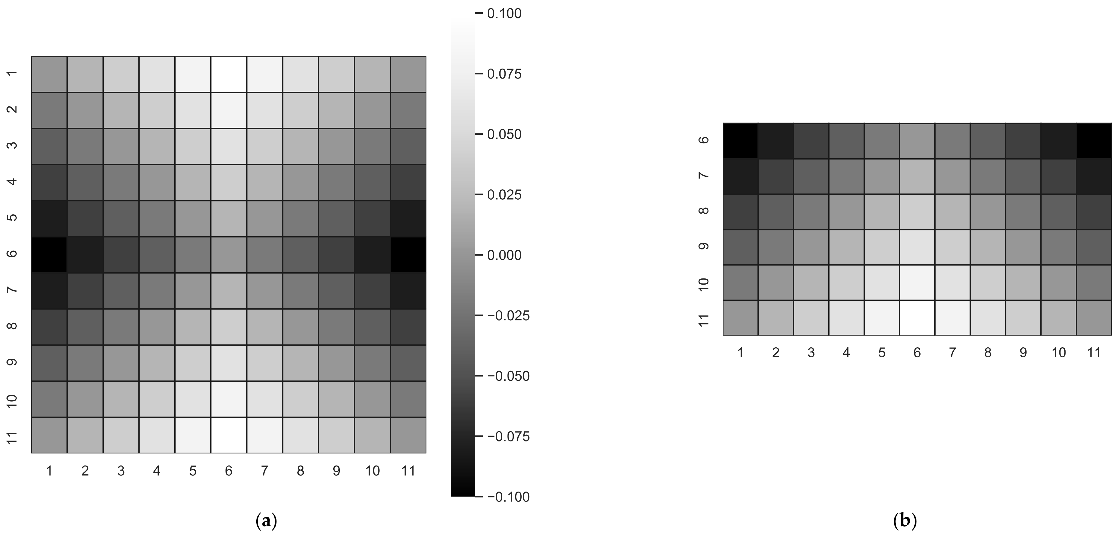
4.2.2. Reward Matrix

When $s_{i,j^{*}}$ increases/decreases in the right/left neighborhood of zero, the operation stability declines. We define a utility function $f_v$, which acquires the maximum value in $s_{i,j^{*}}=0$:

$$f_v\left(s_{i,j^{*}}\right)=-\left|{\widehat{s}}_{i,j^{*}}\right|$$

(12)

Here, we define an odd number $N_s$ and we divide the state into $N_s$ discrete intervals with step ${\delta }_s$ (sec), as we can see in Figure 3. ${\widehat{s}}_{i,j^{*}}$ is the median of the interval in which $s_{i,j^{*}}$ is. The reward matrix $R$ is an $N_s$-order square matrix and represents changes in the utility value resulting from discrete state transitions. $f_v\left({\widehat{s}}_{i,j^{*}+1}\right)-f_v\left({\widehat{s}}_{i,j^{*}}\right)$ of all discrete states constitute the elements of the reward matrix $R$.

With transition to a relatively less stable state, the utility value decreases; otherwise, it increases, as shown in Figure 4a.

4.2.3. Optimal Decision

To alleviate large gaps, buses are guided to speed up their cruising (through guidance to drivers themselves or priority at traffic lights) under the action set $X=\left\{x_1,x_2,\cdots \right\}$ so that they can catch up with preceding buses. On the other hand, improper action may shorten the headway excessively and cause bus bunching. We should take the policy $x^{*}$ with the maximal reward expectation, $\max \left(f_x\right)$, as the speed-up control time $c_{i,j^{*}},$ as seen from Formulas (13) and (14).

$$f_x=\overrightarrow{S}{P}_x^{j^{*}}{\left(\overrightarrow{S}R\right)}^T,x=x_1,x_2,$$

(13)

$$c_{i,j^{*}}=x^{*}=\mathrm{argmax}\left(f_x\right)$$

(14)

$\overrightarrow{S}$ is a probability distribution vector. For example, when $s_{i,j^{*}}\in \left[-9,-3\right]$, bus $i$ is in state 5 according to Figure 3 and $\overrightarrow{S}=\left(0,0,0,0,1,0,\cdots ,0\right)$. The corresponding utility value is $f_v=-\left|{\widehat{s}}_{i,j^{*}}\right|=-\left|\frac{-9+\left(-3\right)}{2}\right|$.

$P_x^{j^{*}}$ is the probability transition matrix of a bus traveling from stop $j^{*}$ to $j^{*}+1$ under the action $x$ and is also an $N_s$-order square matrix. The elements of $P_x^{j^{*}}$ are determined by three factors with a certain $s_{i,j^{*}}$: 1. Arrival rate ${\lambda }_{j^{*}}$; 2. Link travel time $t_{j^{*}}$ from stop $j^{*}$ to $j^{*}+1$; and 3. Speed adjusting action $x\in X$. When speed adjusting is implemented, the link travel time is $t_{j^{*}}+x$. $P_x^{j^{*}}$ is estimated through a stochastic policy—before adopting $x^{*},$ we will let buses choose their action $x\in X$ randomly for several days. It should be noticed that the stochastic policy is also implemented just when $h_{i,j^{*}}>H$. After estimation, $x^{*}$ will be implemented and $P_x^{j^{*}}$ will be renewed using the triple of $\left({\widehat{s}}_{i,j^{*}},x,{\widehat{s}}_{i,j^{*}+1}\right)$ after one day of operation as an episode, ${\widehat{s}}_{i,j^{*}}\in \left(0,+\infty \right)$, ${\widehat{s}}_{i,j^{*}+1}\in \left[-H,+\infty \right)$. By contrast, with the reward matrix $R$, the $\left(\frac{N_s-1}{2}\right)\times N_s$ elements in the upper part of $P_x^{j^{*}}$ are all zero, because the 1^st to $\frac{N_s-1}{2}$ states imply that buses tend to bunch and it is obvious that speed-up control is not necessarily implemented, as shown in Figure 4b. However, the lagging bus may tend to bunch under an excessive speed adjusting action, which is recorded in the $\left(\frac{N_s+1}{2}\right)\times N_s$ elements in the lower part of $P_x^{j^{*}}$.

4.3. Integrated Control

Bus holding control can be implemented at all stops, except the origin and terminal in our study when the bus is approaching the preceding bus ($h_{i,j}<{\alpha }_{1}H$). Speed adjusting can only be implemented at four consecutive stops when $h_{i,j^{*}}>H$ and the policy only involves speed-up action. The process of integrated control strategy is as follows. In Chapter 5, we will discuss which location for the SCP is most beneficial to reducing the passengers’ perceived waiting time according to the demand profiles.

Step 1: Assign a value to ${\alpha }_1$ from $\left\{0.2,0.3,\cdots 1.0\right\}$. Step 2: All buses travel from origin with dispatching interval $H$. When there is a bus $i$ arriving at stop $j$:  Calculate preceding headway $h_{i,j}$.  If $j\ne j^{*}$:   If $h_{i,j}<{\alpha }_{1}H$:    Hold bus $i$ for $H-h_{i,j}+f_{{\alpha }_2}\left(j\right)$ seconds after finishing serving passengers.   Else if $h_{i,j}>H$:    Hold bus $i$ for $\max \left(H-h_{i,j}+f_{{\alpha }_2}\left(j\right),0\right)$ seconds.   Else:    Hold bus $i$ for $f_{{\alpha }_2}\left(j\right)$ seconds.  Else:   If $h_{i,j}<{\alpha }_{1}H$:    Hold bus $i$ for $H-h_{i,j}+f_{{\alpha }_2}\left(j\right)$ seconds after finishing serving passengers.   Else if $h_{i,j}>H$:    If optimal policy is executed:     Calculate state value $s_{i,j^{*}}$ and optimal action $x^{*}=c_{i,j^{*}}=\mathrm{argmax}\left(f_x\right)$.     Guide bus $i$ to travel to stop $j^{*}+1$ in $t_{j^{*}}+c_{i,j^{*}}$ seconds.     Calculate $s_{i,j^{*}+1}$ and renew $P_x^{j^{*}}$ using the triple $\left({\widehat{s}}_{i,j^{*}}, x^{*},{\widehat{s}}_{i,j^{*}+1}\right)$.    Else:     Calculate state value $s_{i,j^{*}}$ and randomly chosen action $x$ from $X$.     Guide bus $i$ to travel to stop $j^{*}+1$ in $t_{j^{*}}+x$ seconds.     Calculate $s_{i,j^{*}+1}$ and renew $P_x^{j^{*}}$ using the triple $\left({\widehat{s}}_{i,j^{*}}, x,{\widehat{s}}_{i,j^{*}+1}\right)$    Else:     Hold bus $i$ for $f_{{\alpha }_2}\left(j\right)$ seconds.  End When every bus finishes a trip from origin to terminal:  Go to Step 3 Step 3:  Output the performance indicators under the present ${\alpha }_1$. Step 4:  If all elements from $\left\{0.2,0.3,\cdots 1.0\right\}$ have been chosen once: End  Else:   Assign the null matrix to $P_x^{j^{*}}$ and a new value to ${\alpha }_1$ which has never been chosen from $\left\{0.2,0.3,\cdots 1.0\right\}$.   Re-execute Step 2‒Step 4.

5. Experiment and Analysis

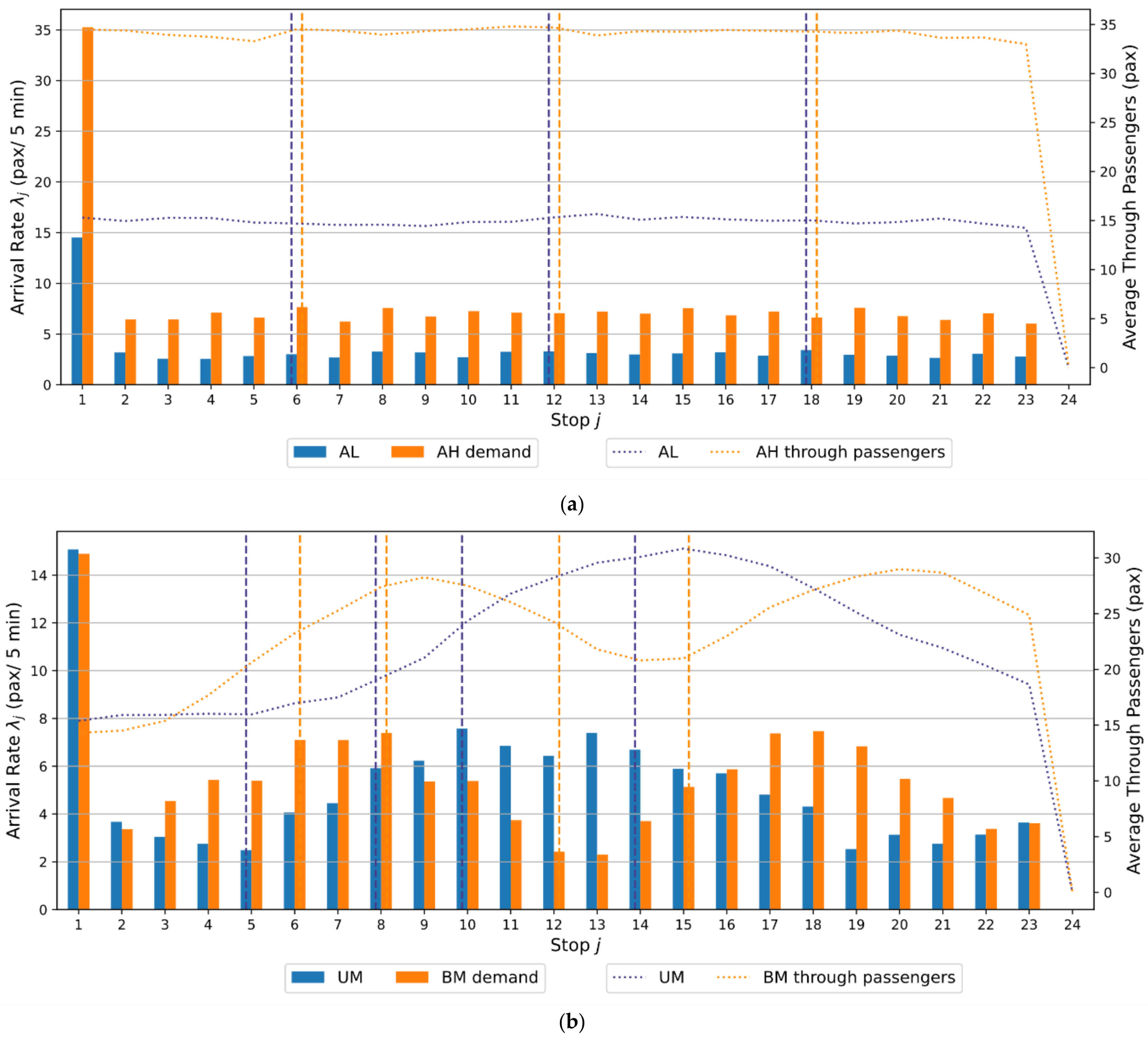
5.1. Simulation Environment and Related Parameters

Our experiments simulate the buses being dispatched from the origin within 1 h on a high-frequency route, with 24 stops and a link length of 500 m. The processes of passenger boarding and alighting occur at the same time. Because buses are dispatched on a high-frequency route, the pattern of passenger arrival can be described to be a uniform distribution [5]. Thus, according to the assumption 1 made in Chapter 3, the model of passenger’ perceived waiting time can be employed on this route. The simulation parameters are shown in

Table 2. Simulation parameters.

Parameter	Value/Characteristic	Explanation
$N$	50 days	Simulation days. Stochastic policy will be implemented for $2N$ days.
$t_j$	Mean: 1.7 min STD: 0.3 min	Travel time of link between stop $j$ and $j+1$. Conforms to lognormal distribution.
$t_{j^{*}}$	Mean: 1.7 min STD: 0.1 min	Travel time of link between stop $j^{*}$ and $j^{*}+1$. Conforms to lognormal distribution.
𝐻	5 min	Dispatching interval.
$p_j^{alight}$	$p_1^{alight}=0$, $p_{24}^{alight}=1$, $p_j^{alight}~U\left[0.1,0.3\right]$, $j=2,3,\cdots ,23$	Alighting rate of passengers from vehicle at stop $j$.
$t^{board}$	4 s/pax	Boarding time per passenger.
$t^{alight}$	2 s/pax	Alighting time per passenger.
$b_1$	0.7	Parameter of waiting expectation.
$b_2$	1.5	Parameter of perceived waiting time.
${\lambda }_j$	See Figure 5.	Passenger arrival rate at stop $j$.
$N_s$	11	Number of discrete states.
${\delta }_s$	6 s	State step.
$X$	$\left\{0,-10,-20,-30\right\}$	Action set of speed adjusting. $t_{j^{*}}+\min \left(X\right)$ must be under road speed limit.

. All link travel times conform to a lognormal distribution [5]. The link travel time of stop $j^{*}$ to $j^{*}+1$ has a lower standard deviation than the general link and it can be regarded as setting dedicated bus lanes, signal priority control, or so as to facilitate bus travel.

We design four profiles of passenger demand: all-low (AL), all-high (AH), unimodal demand (UM), and bimodal demand (BD) in Figure 5. The solid line indicates the arrival rate of passengers per $H=5$ min, and the dashed line is the average through passengers obtained from the average of the arrival and alighting rate.

When choosing the location for the speed adjusting, two extreme cases are considered: If the starting SCP is near the origin, the bus operation is still relatively stable when it arrives at the starting SCP, and outside disturbance has not yet been severe. If the starting SCP is near the terminal, however, the disturbance at the upstream stops of SCPs cannot be effectively controlled. We have chosen several typical stops as the starting SCP for the four profiles of passenger demand (stops 6, 12, and 18 for AL and AH, stops 5, 8, 10, and 14 for UM, and stops 6, 8, 12, and 15 for BM), as shown in Figure 5.

5.2. Performance Indicators

To evaluate the control performance under the current ${\alpha }_1$, ${\alpha }_2$, and the location of the SCP, we introduced two performance indicators. See formulas (15), (16), and (17).

$$W_s={\displaystyle \sum }_{i=1}^{12}{\displaystyle \sum }_{j=2}^{23}\frac{B_{i,j}}{B}{W}_{i,j}$$

(15)

$$W_v={\displaystyle \sum }_{i=1}^{12}{\displaystyle \sum }_{j=2}^{23}\frac{O_{i,j}^d}{O^d}{c}_{i,j}{O}_{i,j}^d$$

(16)

$$W=W_s+W_v$$

(17)

The total number of boarding passengers affected by operation control in a day is $B={\displaystyle \sum }_{i=1}^{12}{{\displaystyle \sum }}_{j=2}^{23}{B}_{i,j}$, and the total number of all affected passengers is $O^d={\displaystyle \sum }_{i=1}^{12}{{\displaystyle \sum }}_{j=2}^{23}{O}_{i,j}^d$. $W_s$ is the weighted waiting time at stops and $W_v$ is the weighted in-vehicle delay. $W$ is the total travel cost.

5.3. Performance Analysis

5.3.1. Influence of Control Strength on Service

In this subchapter, $W_s$, $W_v$, and $W$ (s) are the average values of Formulas (15), (16), and (17) within simulation days $N$. It can be seen from

Table 3. Performance with different ${\alpha }_1$ (UM demand, starting $j^{*}=8$, ${\alpha }_2=0$).

${\mathit{\alpha }}_1$	${\mathit{W}}_{\mathit{s}}$	${\mathit{W}}_{\mathit{v}}$	$\mathit{W}$	${\mathit{\sigma }}_{\mathit{h}}$	${\mathit{n}}_{\mathit{h}>\mathit{H}}$	$\mathit{E}\left(\mathit{h}>\mathit{H}\right)$	${\mathit{\sigma }}_{\mathit{h}>\mathit{H}}$
0.2	1282	−63	1219	97.2	6947	371.5	75.5
0.3	1227	−60	1167	91.3	6921	369.2	69.8
0.4	1231	−44	1187	83.1	6879	362.7	61.4
0.5	1161	−28	1133	82.2	6830	363.7	66.8
0.6	1113	−14	1099	73.5	6685	359.3	58.9
0.7	1085	23	1108	63.7	6875	351.4	52.1
0.8	1064	57	1121	54.5	7277	344.8	44.2
0.9	1049	100	1149	47.4	7810	339.8	40.3
1.0	1059	127	1186	45.7	8149	338.4	40.5

that, as ${\alpha }_1$ increases, buses are held more frequently, and $W_s$ and the standard deviation of headway ${\sigma }_h$ decrease. When ${\alpha }_1\ge 0.9$, the in-vehicle delay $W_v$ increases significantly, offsetting the reduced waiting time by tighter control. In fact, the optimal strength ${\alpha }_1$ in

Table 4. Optimal control strength (${\alpha }_2=0$).

Demand Profile	Starting SCP	${\mathit{\alpha }}_1$	${\mathit{W}}_{\mathit{s}}$	${\mathit{W}}_{\mathit{v}}$	$\mathit{W}$
AL	−	0.6	751	48	799
	6	0.5	644	−23	621
	12	0.5	660	−28	632
	18	0.7	661	1	662
AH	−	0.8	2866	387	3253
	6	0.7	1728	63	1791
	12	0.8	1932	159	2091
	18	0.9	2981	266	3247
UM	−	0.7	1345	153	1498
	5	0.5	1147	19	1166
	8	0.5	1161	−28	1133
	10	0.7	1138	−3	1135
	14	0.7	1243	−15	1228
BM	−	0.7	1535	174	1709
	6	0.6	1271	−13	1258
	8	0.7	1248	15	1263
	12	0.6	1315	28	1343
	15	0.7	1321	7	1328

is not a fixed value but lies in an interval. For example, when starting SCP $j^{*}=8$, the optimal strength ${\alpha }_1$ of UM lies within $\left[0.5,0.8\right]$, seen from Table 3.

As shown in Table 3, greater ${\alpha }_1$ will improve the headway regularity. At the same time, it can be observed that $W_s$ increases when ${\alpha }_1=1.0$. Although tighter holding control can reduce the variation of headway ${\sigma }_h$ (s), and alleviate bus lagging partly from $E\left(h>H\right)$ (s) and ${\sigma }_{h>H}$ (s), the problematic effect is that the lagging frequency $n_{h>H}$ also increases. Along with the model (7) derived in Chapter 3, this phenomenon can be understood as follows: Excessively tight control means that buses have a higher possibility of lagging, and this lagging (large gap) may result immediately in an increase in longer perceived waiting times at the stop under a certain arrival rate. If limited capacity is considered, some passengers will not be able to board the bus and will only choose the next bus when demand is high, and the perceived waiting time may be longer than what is presented in our study. A similar phenomenon can be observed with different profiles and starting SCPs when ${\alpha }_1$ is approaching 1.0; these are not presented here. All profiles benefit from setting SCPs, although speed adjusting control has little influence on the holding control strength indicated in Table 4.

5.3.2. Validity of Speed Adjusting Control

Let us also take the UM profile as an example (starting $j^{*}=8$). The $X$ in the first column of

Table 5. Performance of different speed-up policies (UM demand, starting $j^{*}=8$).

$\mathit{X}$	${\mathit{W}}_{\mathit{s}}$	${\mathit{W}}_{\mathit{v}}$	$\mathit{W}$	${\mathit{W}}_{\mathit{s}}^{*}$	${\mathit{W}}_{\mathit{v}}^{*}$	${\mathit{W}}^{*}$	${\mathit{\sigma }}_{\mathit{h}}$	${\mathit{\sigma }}_{\mathit{h}}^{*}$	$\overline{\mathit{v}} (\mathbf{km}/\mathbf{h})$	$\overline{{\mathit{v}}^{*}} (\mathbf{km}/\mathbf{h})$	${\mathit{p}}_{{\mathit{x}}^{*}}$
0	1530	104	1634	−	−	−	107.39	−	13.91	−	$3\%$
−10	1390	53	1443	1620	−86	1534	98.83	82.08	14.24	14.06	$17\%$
−20	1281	10	1291	1505	−227	1278	91.26	70.34	14.47	14.75	$13\%$
−30	1217	−33	1184	1432	−335	1097	85.37	63.72	14.65	15.33	$67\%$
$x^{*}$	1134	−32	1102	1348	−292	1056	75.80	53.55	14.71	15.06	$100\%$

represents the policy adopted by the lagging bus departing from stop $j^{*}$. “0” means that no SCP is set on the route, and “−10”, “−20”, “−30” are the constant speed-up actions taken by lagging buses departing from stop $j^{*}$. $W_s$ and $W_s^{*}$ are the global/local weighted waiting times, the same as other notations with “$*$”. The column $p_{x^{*}}$ represents the proportion of “0”, “−10”, “−20”, “−30” taken by $x^{*}$ respectively in $N=50$ days.

From Table 4 and Table 5, we can see that when implementing the integrated strategy with all these speed-up policies, the weighted waiting time $W_s$, weighted in-vehicle delay $W_v$, standard deviation ${\sigma }_h$, and cruising speed $\overline{v}$ (km/h) are improved, in contrast to only implementing the holding control. The ‘−30′ policy makes the buses run the fastest in the links after leaving the SCPs and achieves the best local in-vehicle delay $W_v^{*}$ compared with the others. However, the global cruising speed $\overline{v}$ and in-vehicle delay $W_v$ under policy $x^{*}$ are almost the same as ‘−30′, and the global waiting time $W_s$ and standard deviation ${\sigma }_h$ are improved. Compared to the constant policy, $x^{*}$ lets buses avoid some unduly chasing behaviors and thus obtain better service reliability. Appropriate selection of less fast speed-up actions has not aggravated $W_v$ and $\overline{v}$.

All the policies in Table 5 are implemented when $s_{i,j^{*}}>0$. If this restriction is lifted and the bus is allowed to accelerate freely, the faster speed may promote chasing behaviors, which may result in bunching. This gives us insights that if we only ensure the right of the road to allow buses to travel as fast as possible, the space available to other private cars may be occupied and the potential efficiency of transit priority measures may be underutilized.

Now, we alter the number of discrete states $N_s$ and state step ${\delta }_s$ to determine their operational performance in Figure 6 and choose a more unstable demand profile of AH to explore the underlying characteristics of this model (${\alpha }_1=0.7$). All stops, except the origin and terminal, have been selected as SCPs and they consequently share the same $P_x^{j^{*}}$. The new parameters are presented in

Table 6. Parameters of supplementary experiments (${\alpha }_1=0.7$).

Experiment Index	1	2	3	4	5	6
${\delta }_s$ (s)	4	5	6	7	9	11
$N_s$	15	13	11	11	7	7

. Because the speed-up actions are limited, we increase state step ${\delta }_s$ while reducing the number of discrete states $N_s$ to exclude homogeneous states that are far from $s_{i,j^{*}}=0$. In Figure 6, $n_h^{\prime }$ is the times of holding control implemented with different $N_s$ and ${\delta }_s$, compared to the third experiment (holding $n_h$ times). The robustness of the speed adjusting control contributes to satisfactory results when the initial parameters have changed. Moreover, it is recommended to increase ${\delta }_s$ to reduce the homogeneity of states when the maximum executable speed adjusting value becomes larger.

We introduced the linear control of Daganzo [2] and Xuan et al. [3] for speed adjusting in formula (18). The processes of parameter calibration are shown in

Table 7. Parameter calibration of linear control (${\alpha }_1=0.7$).

	${\mathit{\beta }}_2$	0	5	10	15	20
${\mathit{\beta }}_1$
0.4		1128/−9.3%	1043/−5.5%	988/−6.3%	936/+11.6%	934/+25.7%
0.8		989/−9.1%	961/−1.8%	926/+16.6%	911/+19.4%	921/+30.2%
1.2		960/+6.3%	918/+3.0%	932/+4.3%	911/+21.7%	900/+28.5%
1.6		950/+9.1%	921/+13.6%	915/+22.4%	926/+33.5%	928/+39.8%
2		935/+10.6%	941/+8.3%	913/+25.4%	898/+16.9%	889/+24.4%

Explanatory notes: : insufficient control; : proper control; : excessive control. The elements in this table are $W$ and $\frac{n_h^{\prime }-n_h}{n_h}\times 100\%$.

, where $n_h^{\prime }$ is the holding frequency of linear control and $n_h$ is also the frequency of the third experiment in Table 6. We name as ${\beta }_1$ the ratio parameter of $c_{i,j^{*}}$ to $s_{i,j^{*}}$ and ${\beta }_2$ the compensation parameter, by whose value $\left|c_{i,j^{*}}\right|$ is more than $\left|{\beta }_1{s}_{i,j^{*}}\right|$. A larger ${\beta }_1$ means greater feedback to $s_{i,j^{*}}$, and a larger ${\beta }_2$ means an additional reaction to ${\beta }_1{s}_{i,j^{*}}$. On the top-left side of Table 7, linear control yields lower performances and holding frequency, where the speed-up control has not achieved its full utility. On the contrary, on the bottom-right side, excessive speed-up control causes an obviously higher holding frequency and thus causes the buses to tend to bunch up. The estimation of $p_{x^{*}}$ lifts our model from parameter calibration and collects features in the real world automatically. This means that we do not even have to understand the distribution of the link travel time, which is necessary in the works by Daganzo [2] and Xuan et al. [3], and, at the same time, can achieve reasonable control according to Figure 6 and Table 7.

$$c_{i,j^{*}}=max\left[-\left({\beta }_1{s}_{i,j^{*}}+{\beta }_2\right),\min \left(X\right)\right]$$

(18)

5.3.3. Where to Set the Starting SCP

The profiles of AL and AH have constant passenger demand and average through passengers along the route. According to Table 4, their optimal SCP lies in the middle of the route and does not exceed it. On a route like this, SCP selection only needs to consider the distance from the origin and terminal. The optimal locations of the UM profile are at stops 8 and 10, which are close to the peak of demand and through passengers. Stop 14 also lies upstream of stops with a high level of through passengers but too close to terminal, serving fewer passengers at stops. The optimal locations of the BM profile are at stops 6 or 8, which lie behind the first peak of demand. If the second peak is much larger than the first, the optimal location of the SCP will move forward, which may be analogous to the UM.

Proper location of the SCP may offset the in-vehicle delay caused by holding control due to the speed-up action, even though speed adjusting is restricted to be implemented at just a few stops—from stops 6 and 12 of AL, stops 8, 10, and 14 of UM, and stop 6 of BM, according to Table 4. The demand of the real route may not only contain just one profile, but may be composed of the above profiles. Moreover, setting the SCP on the actual line may encounter the challenge that speed control cannot be performed on consecutive links. The discussion of where to set the starting SCP gives us the insight that when selecting the SCP for the real route, the entire route should be divided into multiple sub-routes according to the demand profile, and the optimal control points should be selected for each.

5.3.4. Relationship between SCP and Slack Time

The optimization principle of ${\alpha }_2$ in this experiment is to add as much slack time as possible to reduce the total travel cost $W$. (See the following formulas (19) and (20) for the optimization methods and (21) for the termination conditions.) The slack time is a preset and default holding time, and its length is not calculated in real time from the current headway. Therefore, this study optimizes slack time step by step, without considering the time complexity.

As shown in

Table 8. Performance after adding slack time.

Demand Profile	Starting SCP	${\mathit{\alpha }}_1$	${\mathit{\alpha }}_2$	${\mathit{W}}_{\mathit{s}}^{\prime }$	${\mathit{W}}_{\mathit{v}}^{\prime }$	${\mathit{W}}^{\prime }$	$\frac{{\mathit{W}}^{\prime }-\mathit{W}}{\mathit{W}}\times 100\mathit{\%}$
AL	−	0.6	10	607	88	695	13%
	6	0.5	7	587	15	602	3%
	12	0.5	7	589	5	594	6%
	18	0.7	15	563	101	664	0%
AH	−	0.8	18	1424	467	1891	42%
	6	0.7	13	1339	188	1527	15%
	12	0.8	13	1404	228	1632	22%
	18	0.9	17	1405	338	1743	46%
UM	−	0.7	15	1023	257	1280	15%
	5	0.5	10	998	103	1101	6%
	8	0.5	12	979	86	1065	6%
	10	0.7	10	999	71	1070	6%
	14	0.7	10	1029	69	1098	11%
BM	−	0.7	10	1168	202	1370	20%
	6	0.6	12	1060	105	1165	7%
	8	0.7	10	1085	99	1184	6%
	12	0.6	12	1099	122	1221	9%
	15	0.7	8	1115	74	1189	10%

, in the UM and BM profiles, if sufficient slack time can be guaranteed, $W_s^{\prime }$ is almost the same, but $W_v^{\prime }$ has distinct differences. For profiles that have apparent demand variation, where the platform and road space can fully allow holding control, the main improvement from the SCP is the in-vehicle delay. In Table 8, when the starting SCPs are at stop 14 of UM and at 15 of BM, which lie behind the peak of through passengers, the control performances are also as good as those at the optimal starting SCPs discussed in subchapter 5.3.3.

Comparing $W$ and $W^{\prime }$ of AL or AH, when the starting SCP is placed at stop 6 or 12, satisfactory performance can be obtained even if the slack time ${\alpha }_2=0$. This means that the transit system’s need for slack time can be reduced if SCPs are placed in suitable locations. This is beneficial to the operation of the route where holding control cannot be implemented at all stops due to less need for platform and road space. This conclusion is also true for UM and BM.

We noticed that when the starting SCP of AL is at stop 18, even if adding slack time, its total travel cost $W^{\prime }$ still cannot be reduced effectively. This phenomenon does not appear in AH. When passenger demand is high, bunching and large gaps are more likely to happen. According to the model of passenger perceptions derived in Chapter 3, the longer the waiting time (headway) is or the higher the arrival rate is, the greater the difference between the perceived and actual waiting time will be. Adding slack time to the route or sub-routes with high demand can reduce the perceived waiting time to a greater extent.

$${\alpha }_2=\mathrm{argmin}\left(W\right)$$

(19)

$${\alpha }_2^k-{\alpha }_2^{k-1}={\alpha }_2^{k-1}-{\alpha }_2^{k-2}=\cdots ={\alpha }_2^2-{\alpha }_2^1=1$$

(20)

$$W^k-\min \left(W^1,W^2,\cdots ,W^{k-1}\right)\ge 10\%$$

(21)

6. Conclusions

From the perspective of passenger’s waiting time perceptions, this study proposes an integrated bus holding and speed adjusting strategy to improve bus operation. We assume the waiting expectation for passengers at stops. When the actual waiting time exceeds it, anxiety causes the passengers’ perceived waiting time to differ from the actual waiting time. The greater the difference, the lower the passengers’ satisfaction with the bus service. Passengers may then tend to give up waiting and choose other means of transportation. Therefore, the article establishes a model of passenger perceptions to describe this psychological characteristic quantitatively, which helps to enable bus operation control to meet the actual needs of passengers.

We employ bus holding, based on threshold control, and speed adjusting, based on a Markovian decision model, to alleviate bunching and large gaps, respectively. Several insights are derived:

• Under the circumstances of threshold-based control and considering passenger’s perceived waiting time, tighter strength of holding control can improve the headway regularity and increase the possibility of buses left behind by their preceding buses though, where buses arrive at stops with a larger headway compared to dispatching interval. This side effect may cause the increase of passenger’s perceived waiting time. It gives bus operators the insight that headway regularity should be thought over cautiously. After all, with other control logic, except threshold-based control, the side effect mentioned may occur as well.
• According to the discussion on speed adjusting control in subchapter 5.3.2, making the bus run fast enough can reduce the in-vehicle delay at several stops and increase the local cruising speed, but it may make buses tend to bunch. It is more conducive to improving service reliability to give reasonable speed guidance for buses when large gaps occur, and this will not significantly reduce the average cruising speed along the whole route.
• The starting SCP should be set near the upstream of the peak of demand and through passengers to reduce both in-vehicle delay and passenger waiting times. When the demand profile of the route has apparent variation, considering only through passengers can also achieve satisfactory performance by adding enough slack time. If the starting SCP is properly set, speed adjusting is able to offset some or even all of the in-vehicle delay caused by holding control, and reduce the system’s need for slack time, which means less need for platform and road space where holding control should be implemented.

There are still some deficiencies in this article that need further study in the future. First, when the waiting time of a passenger at a stop exceeds a certain expectation, the passenger’s perceived waiting time is assumed to be a linear function of the actual waiting time, but in fact is not necessarily linear. Second, our study does not consider the impact of real-time information provided by electronic signposts on platforms, mobile terminals, and other equipment on passengers’ tolerance of waiting. Third, the control model of this study contains the pre-specified headway, which is not compared with the effects of self-equalizing and the method with variable headway on the performance in terms of improving passenger’s waiting time perceptions.

References

1. Newell, G.F.; Potts, R.B. Maintaining a Bus Schedule. In Proceedings of the 2nd Australian Road Research Board, Melbourne, Australia, 1 January 1964; pp. 388–393. [Google Scholar]
2. Daganzo, C.F. A Headway-based Approach to Eliminate Bus Bunching: Systematic Analysis and Comparisons. Transp. Res. Part B Methodol. 2009, 43, 913–921. [Google Scholar] [CrossRef]
3. Xuan, Y.; Argote, J.; Daganzo, C.F. Dynamic Bus Holding Strategies for Schedule Reliability: Optimal Linear Control and Performance Analysis. Transp. Res. Part B Methodol. 2011, 45, 1831–1845. [Google Scholar] [CrossRef]
4. Fu, L.; Yan, X. Design and Implementation of Bus Holding Control Strategies with Real-time Information. Transp. Res. Rec. 2002, 1791, 6–12. [Google Scholar] [CrossRef] [Green Version]
5. Cats, O.; Larijani, A.N.; Koutsopoulos, H.N.; Burghout, W. Impacts of Holding Control Strategies on Transit Performance: Bus Simulation Model Analysis. Transp. Res. Rec. 2011, 2216, 51–58. [Google Scholar] [CrossRef] [Green Version]
6. Yin, T.; Zhong, G.; Zhang, J.; Ran, B. A Hybrid Real-time Bus Control Strategy with a Multi-criterion Evaluation. In Proceedings of the 16th COTA International Conference of Transportation Professionals (CICTP 2016), Shanghai, China, 6‒9 July 2016; pp. 681–691. [Google Scholar]
7. Huang, Q.; Jia, B.; Qiang, S.; Xiao, Y. Integrated Bus Control Strategy Considering Holding and Limited-boarding. J. Transp. Sys. Eng. Info. Techno. 2018, 18, 103–109. [Google Scholar] [CrossRef]
8. Chen, W.; Zhou, K.; Chen, C. Real-time Bus Holding Control on a Transit Corridor Based on Multi-agent Reinforcement Learning. In Proceedings of the 2016 IEEE 19th International Conference on Intelligent Transportation Systems (ITSC), Rio de Janeiro, Brazil, 1‒4 November 2016; pp. 100–106. [Google Scholar]
9. Alesiani, F.; Gkiotsalitis, K. Reinforcement Learning-based Bus Holding for High-frequency Services. In Proceedings of the 2018 IEEE 21st International Conference on Intelligent Transportation Systems (ITSC), Maui, HI, USA, 4‒7 November 2018; pp. 3162–3168. [Google Scholar]
10. Bartholdi, J.J., III; Eisenstein, D.D. A Self-coordinating Bus Route to Resist Bus Bunching. Transp. Res. Part B Methodol. 2012, 46, 481–491. [Google Scholar] [CrossRef] [Green Version]
11. Liang, S.; Zhao, S.; Lu, C.; Ma, M. A self-adaptive Method to Equalize Headways: Numerical Analysis and Comparison. Transp. Res. Part B Methodol. 2016, 87, 33–43. [Google Scholar] [CrossRef]
12. Zhang, S.; Lo, H.K. Two-way-looking Self-equalizing Headway Control for Bus Operations. Transp. Res. Part B Methodol. 2018, 110, 280–301. [Google Scholar] [CrossRef]
13. Delgado, F.; Munoz, J.C.; Giesen, R. How Much Can Holding and/or Limiting Boarding Improve Transit Performance. Transp. Res. Part B Methodol. 2012, 46, 1202–1217. [Google Scholar] [CrossRef]
14. Sánchez-Martínez, G.E.; Koutsopoulos, H.N.; Wilson, N.H.M. Real-time Holding Control for High-frequency Transit with Dynamics. Transp. Res. Part B Methodol. 2016, 83, 1–19. [Google Scholar] [CrossRef] [Green Version]
15. Berrebi, S.J.; Hans, E.; Chiabaut, N. Comparing Bus Holding Methods with and without Real-time Predictions. Transp. Res. Part B Methodol. 2018, 87, 197–211. [Google Scholar] [CrossRef] [Green Version]
16. Chen, W.; Wei, X.; Li, Y.; Zhang, H. An Integrated Bus Holding and Limited-boarding Strategy Considering Passengers’ Perception. J. Transp. Sys. Eng. Info. Techno. 2019, 19, 92–98. [Google Scholar] [CrossRef]
17. Wang, J.; Sun, L. Dynamic Holding Control to Avoid Bus Bunching: A Multi-agent Deep Reinforcement Learning Framework. Transp. Res. Part C Emerg. Technol. 2020, 116. [Google Scholar] [CrossRef]
18. Daganzo, C.F.; Pilachowski, J. Reducing Bunching with Bus-to-bus Cooperation. Transp. Res. Part B Methodol. 2011, 45, 267–277. [Google Scholar] [CrossRef] [Green Version]
19. Teng, J.; Jin, W. A Section-speed Guiding Method for Bus Operation Control. J. Tongji Univ. Nat. Sci. 2015, 43, 1194–1199. [Google Scholar] [CrossRef]
20. Yan, H.; Liu, R. Bus Speed Control Strategy and Algorithm Based on Real-time Information. J. Transp. Sys. Eng. Info. Techno. 2018, 18, 61–68. [Google Scholar] [CrossRef]
21. He, S. An Anti-bunching Strategy to Improve Bus Schedule and Headway Reliability by Making Use of the Available Accurate Information. Comput. Ind. Eng. 2015, 85, 17–32. [Google Scholar] [CrossRef]
22. He, S.; Dong, J.; Liang, S.; Yuan, P. An Approach to Improve the Operational Stability of a Bus Line by Adjusting Bus Speeds on the Dedicated Bus Lanes. Transp. Res. Part C Emerg. Technol. 2019, 107, 54–69. [Google Scholar] [CrossRef]
23. Bie, Y.; Xiong, X.; Yan, Y.; Qu, X. Dynamic Headway Control for High-frequency Bus Line Based on Speed Guidance and Intersection Signal Adjustment. Comput. Aided Civil. Infrastruct. Eng. 2020, 35, 4–25. [Google Scholar] [CrossRef]
24. Fan, Y.; Guthrie, A.; Levinson, D. Waiting Time Perceptions at Transit Stops and Stations: Effects of Basic Amenities, Gender, and Security. Transp. Res. Part A Policy Pract. 2016, 88, 251–264. [Google Scholar] [CrossRef]
25. Trompet, M.; Liu, X.; Graham, D.J. Development of Key Performance Indicator to Compare Regularity of Service between Urban Bus Operators. Transp. Res. Rec. 2011, 2216, 33–41. [Google Scholar] [CrossRef] [Green Version]
26. Lv, S.; Tao, L.; Mo, Y. Level of Service Classification and Quantification for Bus Waiting Time on Commuting Trip. J. Transp. Sys. Eng. Info. Techno. 2015, 15, 190–195+221. [Google Scholar] [CrossRef]
27. Teng, J.; Wang, H.; Yang, X.; Liu, H.; Liu, X. Subjective Perception Based on Passenger Congestion Quantification for Bus Operation. China J. Highw. Transp. 2018, 31, 299–307. [Google Scholar] [CrossRef]
28. Mishalani, R.G.; McCord, M.M.; Wirtz, J. Passenger wait Time Perceptions at Bus Stops: Empirical Results and Impact on Evaluating Real-time Bus Arrival Information. J. Public Transp. 2006, 9, 89–106. [Google Scholar] [CrossRef] [Green Version]
29. Herbon, A.; Hadas, Y. Determining Optimal Frequency and Vehicle Capacity for Public Transit Routes: A Generalized Newsvendor Model. Transp. Res. Part B Methodol. 2015, 71, 85–99. [Google Scholar] [CrossRef]
30. Klumpenhouwer, W.; Wirasinghe, S.C. Optimal Time Point Configuration of a Bus Route-A Markovian Approach. Transp. Res. Part B Methodol. 2018, 117, 209–227. [Google Scholar] [CrossRef]
Figure 1. The perceived and actual waiting time ( b 1 = 0.7 , b 2 = 1.5 , λ j = 3 pax/5 min). (a) For individual passenger. (b) For all passengers at the stop.
Sustainability 13 05529 g001aSustainability 13 05529 g001b
Figure 2. Bus traveling from SCP.
Sustainability 13 05529 g002
Figure 3. Discrete interval of state ( N s = 11 , δ s = 6 s).
Sustainability 13 05529 g003
Figure 4. Heatmap of reward matrix. (a) Whole reward matrix. (b) For probability transition matrix.
Sustainability 13 05529 g004
Figure 5. Demand profiles. (a) Profiles of AL and AH. (b) Profiles of UM and BM.
Sustainability 13 05529 g005
Figure 6. Robustness of speed adjusting control ( α 1 = 0.7 ).
Sustainability 13 05529 g006