Framework for Spatial and Temporal Monitoring of Urban Forest and Vegetation Conditions: Case Study Zagreb, Croatia

Abstract

Urban forest and vegetation conditions are an important variable in urban ecosystem management decision-making. However, it is difficult to evaluate and monitor solely on the basis of field measurements. Remote sensing technologies can greatly contribute to the faster extraction and mapping of vegetation health status indicators, on the basis of which agronomy and forestry experts can draw conclusions about the condition of urban vegetation in larger areas. A new remote sensing-based urban forest and vegetation cover monitoring framework is presented and applied to a case study of the city of Zagreb, Croatia. In this study, Sentinel-2 multi-temporal imagery was used to derive and analyze the current state of urban forest cover. Vegetation indices (NDVI, RVI, and GRVI) were calculated. K-means unsupervised classification of the vegetation indices was conducted. In this way, the dimensionality of the vegetation indices was reduced, while all the data contained in it were used to represent their graded values. Vegetation that was in a poor condition stood out better that way. Finally, PCA-based change detection was performed on the vegetation indices graded values, and a map of change was produced. These results need to be interpreted and validated by foresters and agronomists in further research.

1. Introduction

Urban forests and vegetation are of crucial importance for modern towns, because they provide a wide range of ecosystem services that increase citizens’ quality of life. They are also an important part of the urban ecological system, which plays an important role in protecting the urban ecological environment [1]. Vegetation in general has a multitude of urban ecosystem functions [2] and provides multiple benefits for city-dwellers. It makes cities more resilient to atmospheric conditions, sudden climate changes, and the occurrence of thermal islands [3,4,5,6]. The overall urban vegetation inside the city borders (individual trees, parks, and forest communities) affects the physical environment of the city. It aids the selective absorption and reflection of incident radiation and also regulates the exchange of permanent and sensible heat [7,8]. Urban vegetation reduces the potential for creating surface urban heat islands, while the removal of vegetation areas contributes to creating them [9,10]. Furthermore, the spatial distribution and density of forest and vegetation cover within city borders is recognized as a major factor influencing numerous biophysical processes in the urban environment [11,12].

In addition to conventional in situ measurement, which involves sampling by field measurement, satellite multispectral imagery and remote sensing methods can provide an effective, fast insight into the current state of urban vegetation [13,14] over a much larger area without physical contact. Identifying and monitoring the state of (urban) vegetation on land surfaces using remote sensing imagery depends on the spectral signatures of vegetation on multispectral images [15,16]. As a result, spectral variations provide fairly precise spatiotemporal information in monitoring changes in vegetation cover and conditions, often at quantitative levels [17]. The increasing availability of high-resolution satellite images (for example, Sentinel-2) and remote sensing applications for monitoring and assessing urban forest and vegetation areas, provides different options. Remote sensing methods can provide good assessments of vegetation characteristics [18,19,20]. Contemporary remote sensing methods are extremely convenient for forest and urban vegetation information acquisition [21], analysis [22,23], and mapping [24,25]. The authors of [25] concluded that high temporal satellite imagery (for example, Sentinel-2), proved to be an accurate solution for coarse scale vegetation identification and monitoring and showed good acquisition repetitiveness. The spatial resolution of the Sentinel-2 sensor is sufficient to detect significant spatial and temporal variations in urban vegetation [20,26]. It could therefore be useful in urban forest and vegetation management and for assessing its condition and health. Forest health, a more formal, scientific term, is normally used in forestry to describe the forest stand condition [27]. The term appeared in the forestry literature between 1980 and 1990 [28,29], but there was no widely accepted definition for almost 10 years. The authors of [30] integrated definitions of the forest, ecosystem, and health and finally defined forest health as the condition of forest ecosystems that sustains their complexity while providing for human needs [27]. Monitoring urban forest health is very important at the present time, when increased urbanization, climate change, and natural disasters are impacting vegetation negatively [31,32].

While terrestrial evaluation of forest health is time consuming, satellite remote sensing allows low-cost, time effective, continuous monitoring and evaluation of vegetation conditions over large areas [33,34,35]. Optical remote sensing of vegetation (in general) is based on the spectral response of the vegetation. Vegetation spectral characteristics arise from the interaction of solar radiation with cell structure, chlorophyll, and other pigments [36]. The amounts of pigments reflect the damage level, and as the damage level increases, the amount of chlorophyll decreases [37,38,39]. Based on these principles, calculations of vegetation indices have been developed to monitor vegetation condition [40]. Rather than calculating single vegetation indices and their classifications, the current trend in this field favors applying time series and identifying trajectories or functions in datasets [36]. A comprehensive utilization of eight forest change detection algorithms was published by [41]. Landsat satellite scenes have been used for forestry monitoring and analysis for decades [42,43]. Their use increased significantly after the deployment of the free data policy in 2008 [44]. Long-term Landsat missions have enabled the cheap development of long time-series of satellite products, suitable for change detection [43,45,46]. The same data policy was adopted by the ESA for Sentinel data within the Copernicus program [36]. Sentinel optical data, with an even higher spatial resolution, represent a unique data source suitable for forest vegetation monitoring and the assessment of vegetation conditions [39,47,48,49].

In a review paper by [19], the authors stressed the need to recognize the importance of urban forest ecosystems. The need for appropriate installation and sustainable management of urban forests in order to maintain environmental health and improve the quality of urban life was also expressed [50,51]. Successful management of urban vegetation (especially forests) requires timely and accurate information on status, trends, and information on interactions between socio-economic and environmental processes. These processes refer to urban forests that occur in multiple temporal and spatial scales [52,53]. Such information can be obtained by random field sampling and visual interpretation of aerial photographs and in situ measurements. However, these are expensive and mostly labor-intensive and time-consuming procedures, and usually cannot provide full coverage of relatively large areas of interest [54,55]. In contrast, remote sensing (e.g., high-resolution satellite images) has become a useful observational and analytical tool that offers a fast, scalable, and cost-effective way to assess and quantify urban forest dynamics at different spatiotemporal scales [56]. The most common method of remote sensing is the use of vegetation indices and supervised classifications to obtain substrates that are subsequently analyzed in a variety of ways [57,58,59]. The authors of [20] used vegetation indices and a map of LULC changes to isolate and display forest depletion areas in the Bosomtwe Range forest reserve. Similarly, [60] used the classical image classification algorithms, K-mean and ISODATA, for unsupervised classification and the maximum likelihood classification for supervised classification for the purpose of vegetation extraction from remote sensing imagery. In [26], a methodological framework for monitoring changes in the extent and canopy density of forest stands was presented. The supervised classification algorithm and normalized difference vegetation index (NDVI) were combined within a GIS environment to quantify the extent and density change of forest cover stands.

The objective of this paper is to present the framework for spatial and temporal monitoring of urban forest conditions, which relies exclusively on remote sensing methods and can be totally independent of in situ measurements and sensor type. The main idea is to monitor relative changes in the state of urban forest cover over time instead of determining annual changes over large areas using complicated methods [61,62,63]. In this way, trends of the situation in a certain part of the year or the phenological calendar can be monitored and highlighted. In this paper, the preliminary results of the framework for spatiotemporal analysis of urban forest distribution and its condition in the city of Zagreb, Croatia are presented.

In order to detect changes in the state of urban forest cover more effectively, a PCA-based change detection of the results of the classifications was performed. Change detection implies recognizing differences in the representation (current state) of an object or phenomenon by observing it at different times [64]. Timely change detection of features on the Earth’s surface (in our case, urban vegetation) provides a foundation for understanding better relationships and interactions between humans and natural phenomena, in order to obtain additional data and improve decision-making [65].

2. Materials and Methods

2.1. Study Area and Data Sources

Zagreb (45°49′ N, 15°59′ E) is a central European city located in the central part of the Republic of Croatia on the plain bordered by the River Sava to the South and Mt. Medvednica to the North (Figure 1). Its urban area extends along the plain to Medvednica in the South and its slopes in the North. There are individual trees, avenues, parks (in the lowland areas), and forests (Medvednica). The gently sloping hills of Medvednica are covered in forests, and the flat land between Medvednica and the Sava are covered with urban vegetation (grassed areas, shrubs, single trees, and parks). The climate of Zagreb is classified as oceanic with significant continental influences, closely bordering on both a humid continental climate and a humid subtropical climate, with four distinct seasons. Zagreb summers are warm and wet, winters are cold, springs are mild and pleasant with unpredictable weather changes, and autumns are temperate but rainy and foggy during the latter half of the season (Weather Atlas). The city is a densely populated urban area with 792,875 citizens (according to the last population census in 2011), covering an area of 641.36 km². The extent of the study area covers the limits of the city of Zagreb.

2.2. Satellite Data and Preprocessing

Sentinel-2A and 2B (Level-1C, SUHET, 2015) satellite data covering the study area were used to calculate the vegetation indices during the active vegetation period in 2016, 2017, and 2018. The images were acquired at 12 bits in 13 spectral bands at different spatial resolutions. Four were at 10 m (bands: 2, 3, 4, and 8, with central wavelengths of 490.0, 560.0, 665.0, and 842.0 nm and bandwidths of 65, 35, 30, and 115 nm, respectively), six bands were at 20 m (bands: 5, 6, 7, 8a, 11, and 12, with central wavelengths of 705.0, 740.0, 783.0, 865.0, 1610.0, and 2190.0 nm, with bandwidths of 15, 15, 20, 20, 90, and 180 nm, respectively), and three bands were at 60 m spatial resolution (bands: 1, 9, and 10, with central wavelengths of 443.0, 945.0, and 1375.0 nm, with bandwidths of 20, 20, and 30 nm, respectively) [66]. The downloaded Sentinel-2 satellite images were in the WGS84 and UTM (Universal Transvers Mercator) projection. The data obtained in April, July, August, and September in those three years (

Table 1. Details of satellite imagery used in this study.

Year	Month	Day	Satellite
2016	April	26th	Sentinel-2A
	July	12th	Sentinel-2A
	August	14th	Sentinel-2A
	September	23rd	Sentinel-2A
2017	May *	18th	Sentinel-2A
	July	7th	Sentinel-2A
	August	24th	Sentinel-2B
	September	30th	Sentinel-2B
2018	April	28th	Sentinel-2B
	July	5th	Sentinel-2A
	August	9th	Sentinel-2B
	September	28th	Sentinel-2B

* In April, there were no cloud-free images, so the image from May was selected.

) were downloaded from the Copernicus Open Access Hub (https://scihub.copernicus.eu/ accessed on 22 May 2021). Only images with clear sky views of the study area (no or very limited cloud cover) were included in the analysis. As no cloud-free satellite imagery was found for May 2017 and June in all three years of the survey, the data for those months were completely excluded from the analyses in this paper. The exception was April 2017. There was no cloud-free Sentinel-2 sic at the time, so the one from May was used.

Band pre-processing procedures were performed: atmospheric correction, sampling of bands with a resolution of 60 m and 20 m to a resolution of 10 m, and final cutting according to the boundaries of the area of interest. Atmospheric correction of Sentinel-2 bands was performed within the Sentinel Application Platform (SNAP) software package, with the SNAP (Sentinel-2) Toolbox plugin, Sen2Cor, for Atmospheric Correction, using the associated Level-1C product as input. They were atmospherically corrected from Top-Of-Atmosphere (TOA) Level-1C to generate Level-2A (version SNAP 6.0).

2.3. Methods

The methodological framework for spatial and temporal monitoring of changes in urban forest cover is presented in Figure 2. The workflow in this framework consisted of the following steps (Figure 2):

• Calculation of vegetation indices
• Supervised classification for obtaining the urban vegetation (maximum likelihood algorithm was used in this study)
• Unsupervised classification of vegetation indices (NDVI, RVI, GRVI) using the K-means method
• Principal components analysis-based change detection of unsupervised classification results of vegetation indices.

After calculating the vegetation indices, a supervised classification was carried out for the purpose of separating the urban vegetation cover and the urban non-vegetation cover. Based on the classification results, a mask was made (the non-vegetation cover was masked), and only the urban vegetation cover was used for further consideration (Figure 3). Furthermore, the unsupervised classification of vegetation indices (in this case, they are NDVI, Ratio Vegetation Index (RVI), Green–Red Vegetation Index (GRVI)) was used to gradate their values for the purpose of better insight into their dynamics and position on the scene. Finally, the PCA method was implemented on the results of the unsupervised classification of vegetation indices, which further reduced the dimensionality of the data in order to focus attention on the essentials. In this case, this was on problematic areas with the lowest values of vegetation indices. The results were displayed on maps of changes.

2.3.1. Vegetation Indices

Spectral (vegetation) indices are mathematical combinations of different spectral bands of the electromagnetic spectrum, and they are more sensitive than individual bands to vegetation parameters [67,68,69]. They are measures of vegetation activity and are designed to find a functional relationship between vegetation characteristics and remote sensing data [21,27,70]. The main purpose of spectral indices is to enhance the information contained in spectral reflectance data by extracting the variability due to vegetation characteristics, and to minimize soil and atmospheric effects [71]. In this way, the useful ‘satellite’ indicators, which help in determining vegetation health, can be extracted from Sentinel-2 imagery (as in this study). Vegetation indices measure vegetation activity and show the seasonal and spatial variations of green leaves. The main objective of vegetation indices is to enhance and extract the information contained in spectral reflectance remotely-sensed data, by extracting the variability due to vegetation characteristics [71]. Therefore, they are suitable for detecting within-field spatial variability [70].

In this study, three vegetation indices in the process of monitoring the urban forest condition were used: NDVI, RVI, and GRVI. NDVI [40,72] is the most common vegetation index, and it represents the ratio of the NIR and red band (

Table 2. Vegetation indices derived from Sentinel-2 imagery.

Vegetation Indices	General Formula	Formula with Sentinel-2 Bands
NDVI	$NDVI=\left(\frac{R_{NIR}-R_{red}}{R_{NIR}+R_{red}}\right)$	$NDVI=\left(\frac{B_8-B_4}{B_8+B_4}\right)$
RVI	$RVI=\frac{R_{NIR}}{R_{red}}$	$RVI=\frac{B_8}{B_4}$
GRVI	$GRVI=\frac{R_{NIR}}{R_{green}}$	$GRVI=\frac{B_8}{B_3}$

). It is used for calculation because the absorption by chlorophyll of these two bands of the electromagnetic spectrum is the highest [73]. NDVI was calculated using the (Sentinel-2) red (B4) and near-infrared (B8) bands. A common practice in remote sensing is the use of band ratios to eliminate various albedo effects. If RVI is used [40,74] (Table 2), the vegetation isoline converges at the origin. It is calculated using the (Sentinel-2) red (B4) and near-infrared (B8) bands. GRVI [75] (Table 2) was chosen because it is sensitive to photosynthetic rates in forest canopies, as green and red reflectance are strongly influenced by changes in leaf pigments. It was calculated using the (Sentinel-2) green (B3) and near-infrared (B8) channels.

2.3.2. Urban Vegetation Supervised Classification and Mask

Urban vegetation cover classification was conducted using Sentinel-2 imagery from April, July, August, and September 2016, 2017, and 2018 using the maximum likelihood classification algorithm in QGIS with the semi-automatic classification plugin. The maximum likelihood [76] algorithm calculates the probability distributions for the classes, related to Bayes’ theorem, estimating if a pixel belongs to a land cover class. In particular, the probability distributions for the classes assumed the form of multivariate normal models [77]. The sole purpose of this classification was to determine the area covered by vegetation within the administrative boundaries of the city of Zagreb.

2.3.3. Unsupervised Classification of Vegetation Indices

Unsupervised classification [77] attempts to find clusters in an n-dimensional feature space and assigns those clusters to a group. Samples are not required, and it is an easy way of segmenting and understanding an image. In this case, representations of the distribution of the values of the vegetation indexes for the selected dates were made (Table 1) based on K-means unsupervised classification [78]. K-means unsupervised classification calculates initial class means evenly distributed in the data (feature) space, then iteratively clusters the pixels into the nearest class using a minimum distance technique [79]. This algorithm aims at minimizing a squared error function [78], and it can be expressed by Equation (1) [78]:

$$J={\displaystyle \sum }_{j=1}^k{\displaystyle \sum }_{i=1}^n{\Vert x_i^{\left(j\right)}-c_j\Vert }^2$$

(1)

where:

• ${\Vert x_i^{\left(j\right)}-c_j\Vert }^2=$ chosen distance measure between a data point $x_i^{\left(j\right)}$ and the cluster centre $c_j$,
• $x_i^{\left(j\right)}=$ data point,
• $c_j=$ cluster center,
• n = data points, and
• k = number of class.

The goal of K-means is to reduce the variability within the cluster (class). Thus, areas with similar values of vegetation can be separated and better represented (by grading index values), and a better insight can be gained into the distribution (spatial component) of the indices. Unsupervised classifications of vegetation indices have been carried out for the purpose of grading their values and distinguishing different vegetation conditions in assessing urban forest and vegetation health.

2.3.4. Principal Components Analysis-Based Change Detection

Principal components analysis (PCA)-based urban forest change detection and analysis using the results of unsupervised classification of vegetation indices derived from multitemporal satellite data was performed and is described in this paper. The PCA method has been commonly used for many years to determine the basic dimension of satellite images [80,81,82], land-cover change detection [83,84], or multitemporal satellite data [81,85,86]. Due to its simplicity and capability of enhancing the information on change, it has become one of the most popular change detection techniques [87,88]. PCA is used when it is assumed that multitemporal data are highly related and that information about changes can be highlighted in new components [65]. Compared to projecting data onto the original coordinates, projecting onto the PCs has the advantage of allowing it to detect changes in data correlation which cannot be detected in the original individual variables. Furthermore, this can ensure that any changes to the source variables will be reflected in the PC projections [82]. In the case described in this paper, the input data for PCA were the results of unsupervised classifications of three (GRVI, NDVI, RVI) vegetation indices for the months of May, July, August, and September 2017. The main idea of using PCA was to identify a set of orthogonal principal components from the original feature space, which would better represent the data in the new space. In other words, changes in the different health conditions of urban forest areas were highlighted. This provided the basic prerequisite for detecting changes in the area of interest: the availability of imagery from two or more different dates [85].

3. Results and Discussion

The main idea of this framework is to fully rely on remote sensing methods for the purpose of monitoring urban forest cover, the dynamics of changes in it, and detecting areas with the lowest values of vegetation indices. In this way, trends in the condition of this cover can be followed over time. Compared to the in situ trait approach, remote sensing sensors are unable to detect all traits and trait variations [89] except for some, such as biochemical–biophysical, physiognomic, morphological, structural, and functional traits at all levels of biotic organization, based on the principles of image spectroscopy across the electro-magnetic spectrum [90,91]. Remote sensing sensors can record the status, stress, disturbances, or resource limitations of vegetation over the short and long term on local and global scales [91,92]. These facts were used in creating this framework. The relative relations of the condition of the same species in the same time period are the main indicators for the work of experts in the field of agronomy, forestry, and urban planning. Namely, noticing bad trends in the state of urban forests is a trigger for experts in terms of taking action to prevent such a trend. After noticing such trends, they can go out into the field to perform in situ measurements and additional analyzes to gain insight into the absolute state of vegetation cover and take actions to mitigate or eliminate the problem.

The paper presents the unsupervised classification of vegetation indices as a novel way of presenting the values that can serve as an indicator for assessing vegetation health status. Since each of the spectral indices presents vegetation in a different way, it might be described as a kind of data fusion for improving their usage and information. This paper focuses on representations of remote sensing methods and their preliminary analysis. Forestry experts’ interpretations of the results were not included in this review and are necessary in further research.

3.1. Supervised Classification Outputs

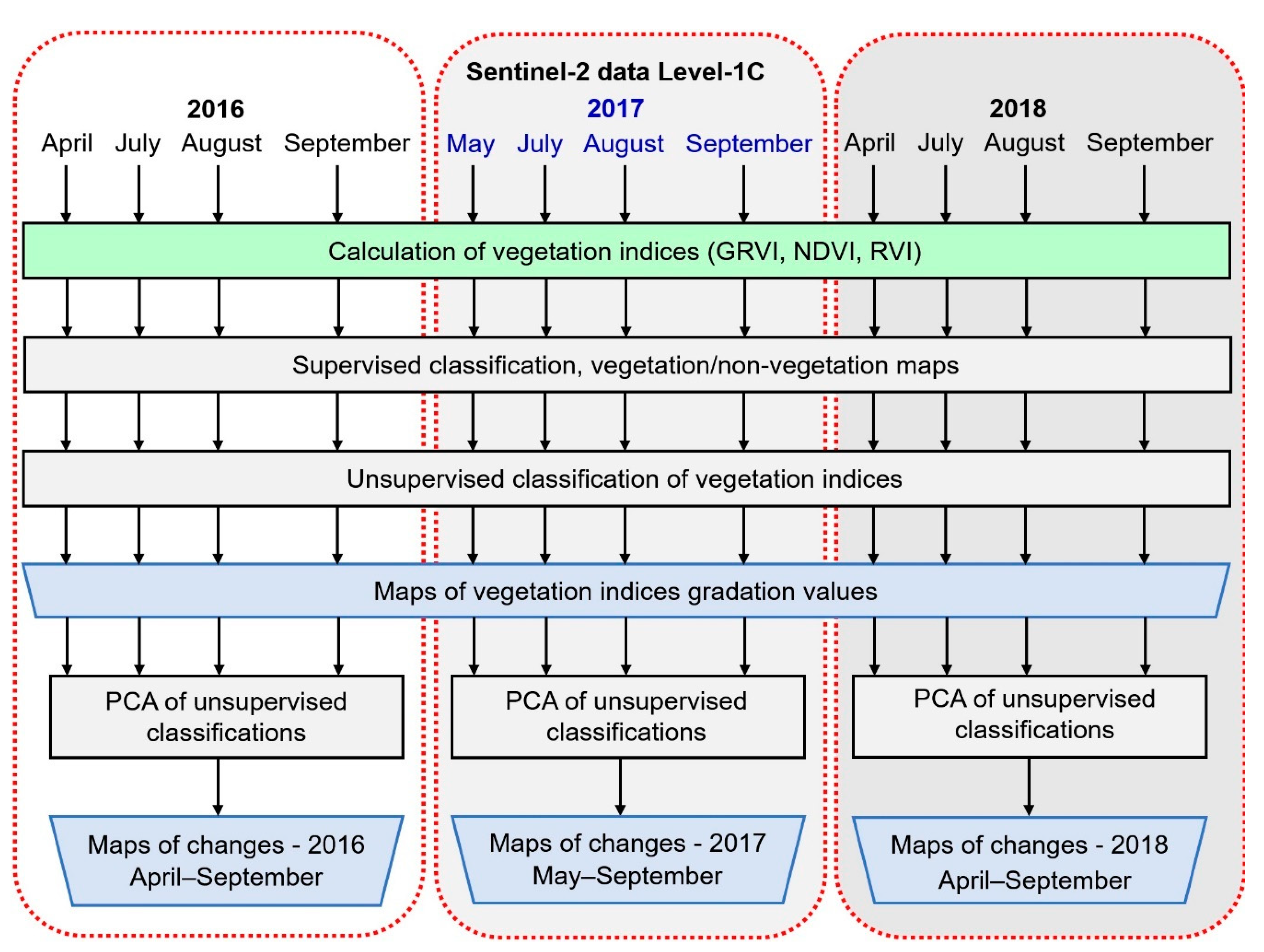
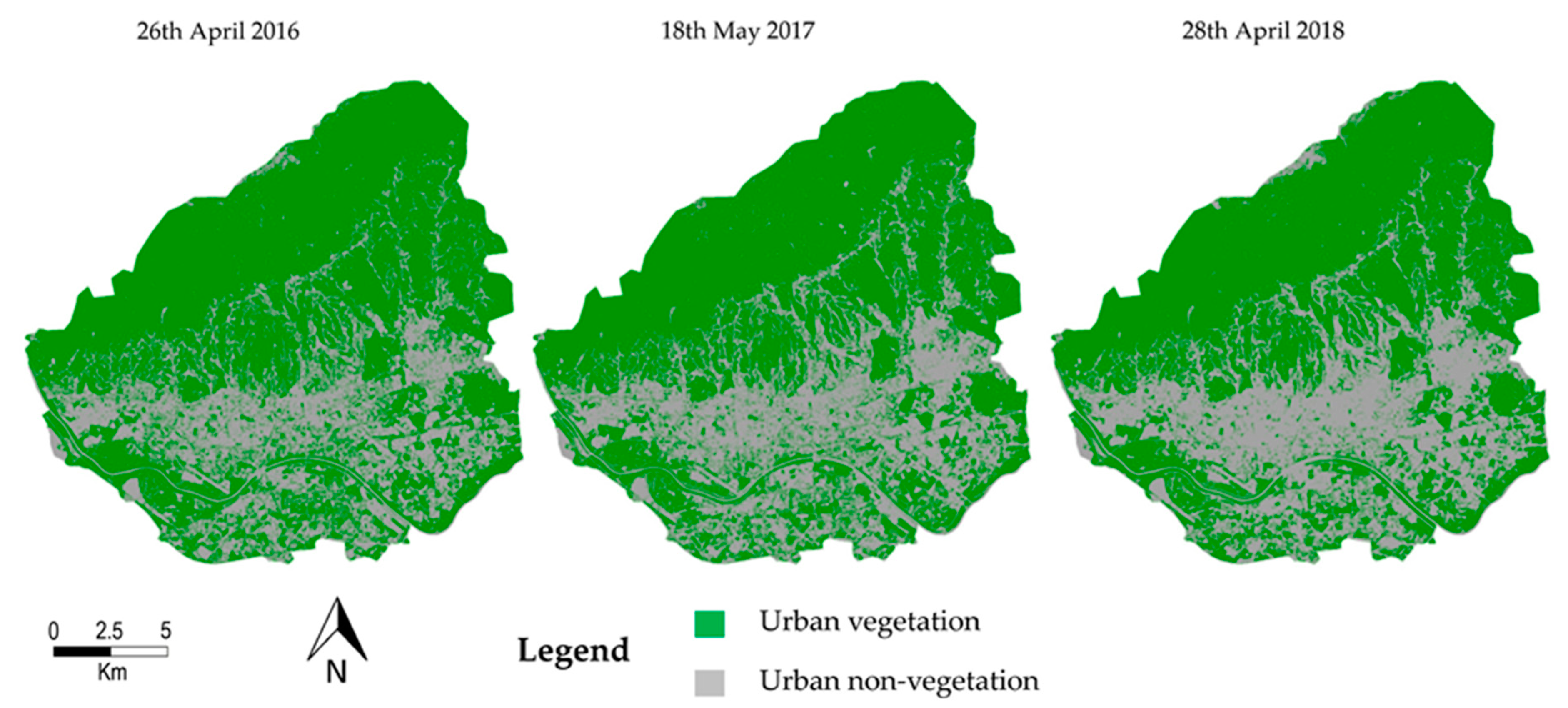
Class samples were visually selected urban vegetation (all types: grassed areas, shrubs, trees, agricultural land) and urban non-vegetation polygons (built-up areas, bare land, and water). The pixels inside the sample polygons were used to perform the classification of each Sentinel-2 set of bands (only bands 2, 3, 4, 5, 6, 7, 8, and 8a, with 10 and 20 m spatial resolution and all vegetation indices were used for supervised classification) and for each date (a total of 12 classifications). The accuracy of vegetation cover classification ranged from 95 to 97%. Selected time series Sentinel-2 imagery was then clipped to the city administrative boundary (Figure 3). The urban vegetation cover was extracted by merging all vegetation classes in one class, and all other areas were merged in a second class (urban non-vegetation) with no data value attached. All further processing was carried out only on the surface covered by urban vegetation.

The results of the classifications were averaged over the years and showed the decrease in the urban vegetation and increase in the non-vegetation cover in the city of Zagreb from year to year (

Table 3. Average results (by year) of the supervised classification.

Year	Vegetation Cover (Square Kilometer)	Urban Vegetation Percentage	Urban Non-Vegetation Percentage	Percentage of Degradation
2016	201.7	65.2	34.8
2017	196.9	63.6	36.4	1.6
2018	187.7	60.6	39.4	3.0

).

3.2. Vegetation Indices Analysis

The value of NDVI ranged from −1 to 1; however, because the value ranges for RVI and GRVI depended on the pixel values in the channels used, there were no fixed ranges.

The NDVI (Figure 4,

Table 4. Overview and statistics of calculated vegetation indices [93].

Year	Month	Mean Value	Min	Max	Standard Deviation	Index
2016	April	0.790	0.212	0.911	0.104	NDVI
	July	0.782	0.290	0.916	0.096
	August	0.782	0.239	0.931	0.117
	September	0.723	0.251	0.901	0.097
2017	May	0.803	0.200	0.918	0.096
	July	0.776	0.183	0.938	0.129
	August	0.770	0.225	0.911	0.111
	September	0.740	0.159	0.897	0.093
2018	April	0.828	0.428	0.929	0.077
	July	0.825	0.343	0.928	0.065
	August	0.739	0.257	0.903	0.099
	September	0.743	0.300	0.900	0.096
2016	April	10.450	1.538	21.588	4.328	RVI
	July	9.648	1.819	22.811	3.655
	August	10.454	1.630	27.785	4.625
	September	7.014	1.670	19.267	2.472
2017	May	10.993	1.499	23.539	4.303
	July	10.791	1.447	27.542	5.630
	August	9.512	1.582	21.577	4.079
	September	7.560	1.379	18.408	2.581
2018	April	12.725	2.494	27.132	5.187
	July	11.651	2.042	26.913	3.645
	August	7.650	1.693	19.606	2.823
	September	7.776	1.857	18.970	2.867
2016	April	6.786	1.853	12.371	1.712	GRVI
	July	7.249	2.113	13.737	2.148
	August	7.952	1.891	17.730	2.830
	September	5.757	1.788	13.018	1.599
2017	May	7.421	1.459	13.405	1.982
	July	8.797	1.927	21.262	3.594
	August	7.493	1.775	15.692	2.444
	September	5.930	1.546	12.210	1.547
2018	April	8.421	2.890	16.278	2.065
	July	8.261	2.202	15.194	2.187
	August	5.971	2.076	12.481	1.742
	September	6.238	2.054	13.952	1.767

) scale varied within a range from 0.183 to 0.938, where the standard deviations were of the smallest scale in comparison to the three indices used; therefore, the smallest variable of the vegetative coverage at the scene is shown. Although the NDVI detected water bodies and bare soil (non-vegetation areas), it did not distinguish forest and domestic vegetation types, so it was not suitable for classifying areas with dense green vegetation. By analyzing the averaged mean values (Figure 5a,b), it was confirmed that the NDVI had very similar seasonal variations along with the middle values of the RVI, because both depend on the values of the same spectral channels, i.e., red and near-infrared. By observing the mean values, it was noticeable that they continuously decreased in 2017 (May to September), whereas in 2016, the value was almost constant until August, when it radically decreased. In 2018, there was a significant decline in the value between July and August (Figure 5c). Scrutinizing the absolute minimum, variation on a much bigger scale was noticeable, which points to the enlarged capability of the NDVI regarding the recognition and gradation of poor vegetation. In contrast, analyzing the maximum showed much less variation, which points to the familiar trait of satiation of the NDVI, i.e., its reduced ability to extract details from areas of thriving vegetation.

The span of RVI values (Figure 4, Table 4) was the highest in comparison to the two other indexes in the observed period from 2016 to 2018 (1.447–27.785). One consequence of this was the highest values of standard deviation, meaning that this index displayed the highest variability of vegetation cover. When analyzing the averaged mean values, it was noticeable that they continuously decreased in 2017 (although with a milder decline than NDVI). The values recorded in 2016 also produced similar results; the values were similar in April and August, while those in July were smaller. There was also a continuous drop of values in 2018, with a radical decrease between July and August (Figure 5d). Minimum values were approximately constant during all the observed months. Maximum values, however, varied much more, with a radical increase in August 2016 (27.785). The maximum values of RVIs during 2018 followed a similar trend as the corresponding average values. Similar maximum values were recorded during April and July (about 27) and August and September (about 19). April, on average, represented the period of local maximum vegetation. As the months of May and June were not included in this survey, the exact appearance of the average curve could not be determined for the indicated period. However, there was a slight decrease in vegetation intensity between April and July. The annual decline in mean RVI began in August and was further compounded by the climatological arrival of autumn in September.

The value range of GRVI (Figure 4, Table 4) was slightly smaller than for RVI (1.459–21.262). The middle and extreme GRVI values were generally lower than the corresponding RVI values. This was a consequence of the fact that the leaves of healthy vegetation reflect green radiation more strongly than red. Accordingly, the ratio between reflected infrared and green radiation was lower than the ratio of reflected infrared and red radiation. With this index, mean values increased continuously from April to August 2016 and then rapidly decreased. The same was true in 2017, with growth from May to July and then a continuous decrease until September. In 2018, the decreases occurred in steps (Figure 5e). At the maximum, greater variation was observed than at the minimum. The GRVI effectively diagnosed the distributions of agricultural vegetation and forest areas, but often failed to discern cropland (at the edges of the city’s southern borders).

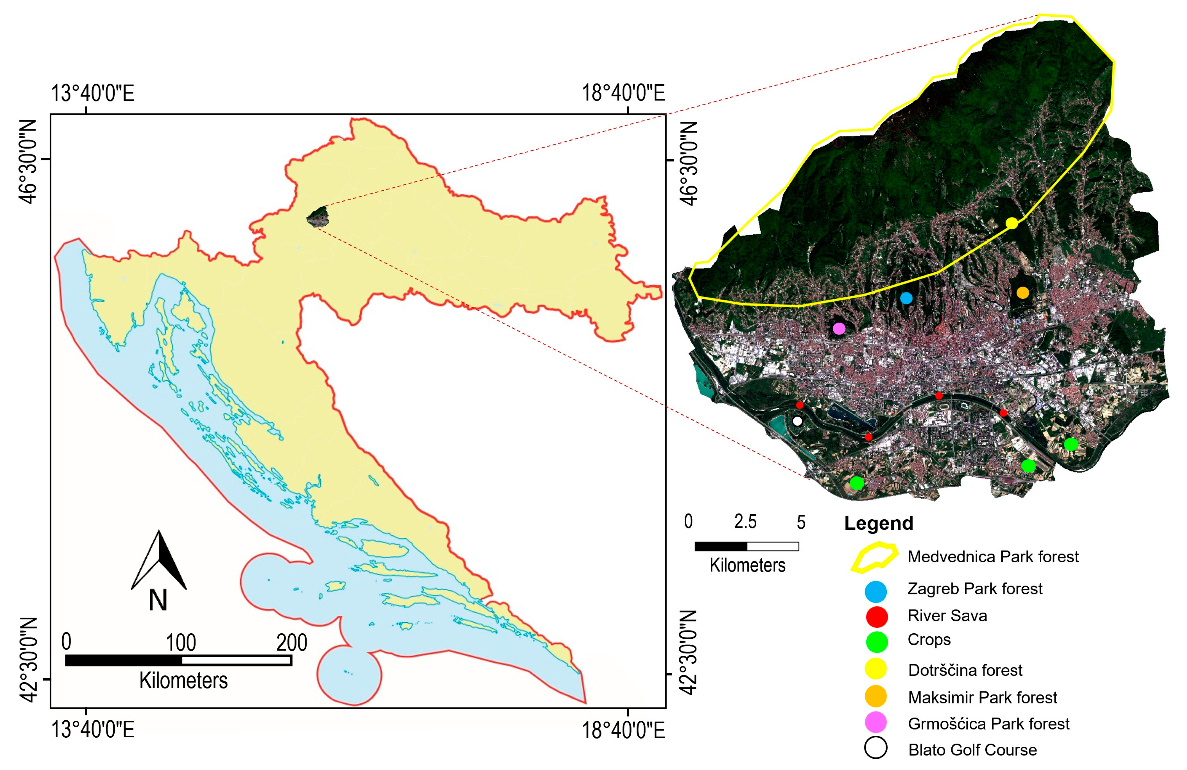
A more detailed analysis was conducted at two locations of special importance for the residents of the City of Zagreb: Maksimir Park (Figure 1, ocher dot) and Dotrščina forest (Figure 1, yellow dot). Maksimir Park is the most popular, oldest park in Zagreb. It is located in the Eastern part, not far from the city center. In addition to five lakes, it contains many plant species, among which are century-old oak trees, which were necessarily prominent. Maksimir Park is known as the ‘lungs of the city’ because it produces oxygen and acts as a natural air purifier. The dominant deciduous species in Maksimir Park are pedunculate oak (Quercus robur), sessile oak (Quercus petraea), and chestnut (Castanea sativa). The dominant coniferous species are white and black pine (Pinus sylvestris and Pinus nigra) and spruce (Picea excelsa) within the oak forests. Dotršćina forest is located north of Maksimir Park on the slopes of Mt. Medvednica. Thus, the analysis focused on predominantly forest vegetation in the lowland, densely populated city center and the hilly, sparsely populated part of the city.

The objects of the analysis were the vegetation indices values of GRVI, NDVI, and RVI for the forest areas in Maksimir Park and Dotrščina forest for May, July, August, and September 2017 (Figure 6). The hypothesis was that RVI has the greatest variability in the presentation of vegetation conditions (largest standard deviations) and that NDVI has the smallest, and this was confirmed in these areas (Figure 6). The highest values of GRVI were measured in July in Maksimir Park, and in May in Dotrščina forest. The highest values of RVI and NDVI were measured in May 2017 in both areas (Figure 6).

These and similar analyzes can be found in the published articles mentioned in the Introduction. In contrast to such analyzes, in this framework, these results were used to produce new results, with existing tools (unsupervised classification and PCA method), which would indicate potential problems in urban vegetation cover. Unsupervised classification of vegetation indices provides insight into the spatial distribution of their values and conducts their gradation.

3.3. Unsupervised Classification Outputs

The input data for the unsupervised classification were vegetation index sets (NDVI, RVI, and GRVI) for each of the dates listed in Table 1. A total of 12 classifications were conducted. The urban vegetation cover in the city of Zagreb was graded into four classes, whereby the class indicated by the lightest green (vegetation 1) represented the maximum value of vegetation indices, while the class indicated by the darkest green (vegetation 4) represented the minimum value of vegetation indices (Figure 7). The unsupervised classification procedure was performed separately for each set of vegetation indices respectively. Therefore, the four classes within the vegetation were not absolutely defined, but rather represented the relative gradation of the index values for each individual set.

The relative maximum value of classified values of vegetation indices during April was found on the middle and low slopes of Medvednica and in the Zagreb forest park at the foot of the mountain. The maximum value of classified vegetation indices during this period also occurred on the banks of the River Sava and on certain cultivated vegetation areas. The minimum values during April usually occurred in the highest regions of Medvednica, in individual areas of arable land, and in the Blato golf course. Between April and July, the relative maximum of classified values of vegetation indices moved almost exclusively to the middle and high regions of Medvednica. The lowest parts of Medvednica and the Zagreb forest park (the sites of the most intensive vegetation in the middle of spring) were then predominantly allocated to vegetation class 2 (medium intensity vegetation class). The minimum value of classified values of vegetation indices during July mostly occurred in meadow areas, including the banks of the Sava. No major changes in the urban vegetation appearance of the city of Zagreb were detected between July and August in the analyzed period. Maximum values of classified values of vegetation indices continued to prevail in Medvednica, while minimum values occurred in areas of low vegetation within the inner city. In the Zagreb forest park areas, there was greater diversity during September, while in other vegetation areas (landscaped parks, low vegetation, cultivated areas), no significant changes were observed in this period regarding the results of unsupervised classification. Between August and September, an increasing number of changes in the results of unsupervised classification of vegetation indices began to occur. The maximum value of classified values of vegetation indices was still predominantly found on Medvednica; however, the overall picture changed or became more varied (different vegetation classes appeared). An increasing number of dark spots (islands of poor vegetation) began to appear in the area of the mountain within the area of stronger vegetation. During September, the value of classified vegetation indices in the forest areas in the highest parts of the mountain also decreased.

The analysis of the unsupervised classifications results of forest cover in the Maksimir and Dotrščina locations revealed that the highest values of vegetation indices were measured in May 2017, and the lowest were in September, for both areas (Figure 8). Most of the forest cover in both locations was classified into class 2. However, apart from in May, when the ratio was almost 1: 1 (D = 69.2% and M = 70.9%), in all other months, the ratio was significantly in favor of the Dotrščina location (July 92.6/52.2%; August 81.9/68%; and September 76.8/36.3%, Figure 9). Furthermore, at the Dotrščina location, significant values (apart from in May) classified into class 1 (maximum index values) appeared in each observed month, while those at the Maksimir location were insignificant, with the exception of May (

Table 5. Class coverage statistics for Maksimir and Dotrščina vegetation cover.

Maksimir–Class Coverage Statistics
2017	May		July		August		September
Class	Pixel	%	Pixel	%	Pixel	%	Pixel	%
1	1336	7.63	4	0.02	80	0.46	84	0.48
2	12,410	70.90	9146	52.19	11,911	67.97	6368	36.35
3	2792	15.95	7238	41.30	5155	29.42	9286	53.01
4	965	5.51	1137	6.49	1012	5.77	1781	10.17
Dotrščina–class coverage statistics
2017	May		July		August		September
Class	Pixel	%	Pixel	%	Pixel	%	Pixel	%
1	5327	18.6	470	1.6	3767	13.1	2504	8.7
2	19,828	69.2	26,598	92.6	23,514	81.9	21,967	76.8
3	3149	11.0	1282	4.5	1109	3.9	3712	13.0
4	344	1.2	368	1.3	324	1.1	436	1.5

). The trend of the mean movement was very similar, and the standard deviations were inversely proportional to the mean values for both locations (Figure 10). The standard deviations were similar in May and September, and differed significantly in July and August. While the standard deviations were uniform for the Dotrščina location, the standard deviations for the Maksimir location were significantly higher in July and August. Therefore, greater variability of the vegetation cover condition was detected in the Maksimir location (Figure 10).

3.4. Principal Components Analysis of Unsupervised Classification Outputs

PCA was used to extract useful information from unsupervised classifications of vegetation indices and detect temporal changes in the current state of forest cover and creation of map changes. The principle of extracting information in this way is described for Maksimir Park and Dotrščina forest for May, July, August, and September 2017.

After transformation of the original images (unsupervised classifications), four principal components of each area were created. The first component showed the largest possible differences in variance (

Table 6. PCA statistics for Maksimir and Dotrščina locations.

	Maksimir	Dotrščina	Maksimir	Dotrščina
	Correlation Coefficient		Percentages of Variance
	PC1
Class_May	0.7736	0.9104	43.0955	51.7349
Class_July	0.1660	−0.3711	27.2206	27.6029
Class_Aug	0.9612	0.4955	20.0204	11.0605
Class_Sept	0.2106	0.4551	9.6635	9.6018

). However, the other components also showed significant percentages of variance (Table 6). The vegetation indices value change map derived by PCA is shown in Figure 11. In the change maps, changes of vegetation indices values were detected and identified at the Maksimir and Dotrščina locations. These maps were created by merging the first three main components in an RGB display: R = PC3, G = PC2, B = PC1. Thus, the changes that occurred from May to September 2017 were highlighted (Figure 11). Areas where changes occurred were marked from light pink to darker shades in both cases (Figure 11). The observed changes are related, among other things, to significant damage to oak trees. Namely, during 2017, oak lace bug (Corythucha arcuata) spread throughout the entire area pedunculate oak and sessile oak (Figure 11).

The data processed and presented by the maps of changes are intended for experts in forestry, agronomy, and urbanism for the purpose of monitoring the state of change in the urban forest/vegetation cover and making adequate decisions in the management of these fragile urban resources.

4. Conclusions

Urban and forest health assessments are very important in the formulation of ecosystem management strategies as well as managing the quality of life in cities. However, the lack of rapid, cost-effective, and quantitative analyses of the health of urban forests and vegetation hinders timely insights into the relative health status of urban vegetation. It was the motivation to create this framework entirely based on remote sensing. The described framework is a closed cost-effective system that uses free satellite images (funded by European states and free delivered by the European agency), free software (open source), and provides insight into the relative trends of the value of vegetation indices and shows their spatial distribution. In this way, spatial and temporal monitoring of changes within the urban forest and vegetation cover was performed, and insight into the trends of these changes was gained. Furthermore, the areas with the highest and lowest values of vegetation indices were also highlighted. The results of these analyses and assessments of these changes need to be delivered to the experts, and they can determine their impact on environmental and human health and take action based on them. Thus, the results of the methodology within this framework are the input data for decision support systems for the purpose of urban forest and vegetation management.

In this case study, Sentinel-2 time series data were used to derive combined vegetation indices for an urban forest and vegetation analysis. Variations in the values of three vegetation indices, NDVI, RVI, and GRVI, in the months of April, July, August, and September from 2016 to 2018, were analyzed. An analysis of the mean values revealed that the vegetation condition depended on the month of observation. All the vegetation indices had the highest mean values in April and increased from year to year. The RVI had the highest perennial average in April (11.4), and during July (10.7), August (9.2) and September (7.4), it recorded a gradual fall in mean values. The NDVI behaved similarly to the RVI, with mean values peaking in April (0.807) and declining in July (0.794), August (0.764), and September (0.735). The GRVI took into account the records of the green spectral channel and, therefore, provided a somewhat different insight into the annual course of vegetation. The GRVI perennial average rose between April (7.5) and July (8.1) and fell during August (7.1) and September (6.0). These data are numerical and represent the result of measurements, but they are still estimates because they were obtained from remote sensing data, without in situ measurements that would confirm or refute them. Therefore, visualizing these assessments gives a better insight into the situation on the scene and indicates problem areas. Temporal data, on the other hand, provide insight into the trends of these problems. In this way, changes in vegetation cover can be more easily detected and visualized. After that, the attention of experts can be focused on problem areas where in situ measurements can be performed and decisions can be made based on them.

The analysis of the unsupervised classification results of vegetation indices showed that the condition of urban vegetation in the city of Zagreb depended on vegetation type, altitude, and the location of the vegetation within the city. The values of 36 spectral indices were combined to yield 12 new results by unsupervised classification. Thus, the dimensionality of the input data was reduced, and all the data contained in the spectral indices were used to display their gradation values. These reduced data were further analyzed by the PCA method in order to determine the trend of changes in the urban vegetation cover. Therefore, this research presented a remote sensing-based monitoring source with the potential to analyze continuous changes in urban forests and vegetation, and assist expert decision-makers in agronomy and forestry to develop ecosystem services management plans. This framework of spectral indices provides indicators for the rapid, cost-effective, and quantitative assessment of forest health. For the operational assessment of the proposed framework of combining spectral indices by unsupervised classification, for the purpose of obtaining indicators for assessing the condition and health of urban forests and vegetation, the results obtained should be compared with reference field data, and their interpretation should involve agronomy and forestry. Further research should be directed in the direction of using other vegetation indices and professional (forester, agronomist) interpretation of the obtained results.

References

1. Wenze, Z.; Haochuan, L. Urban vegetation coverage monitoring technology based on NDVI. In Advances in Engineering Research, Proceedings of 7th International Conference on Energy, Environment and Sustainable Development (ICEESD 2018), Shenzhen, China, 30–31 March 2018; Kim, Y.H., Ed.; Atlantis Science Co. Ltd.: Beijing, China, 2018; Volume 163, ISSN 2352-5401; ISBN 978-94-6252-503-0. [Google Scholar]
2. Bolund, P.; Hunhammar, S. Ecosystem services in urban areas. Ecol. Econ. 1999, 29, 293–301. [Google Scholar] [CrossRef]
3. Bernatzky, A. The contribution of trees and green spaces to a town climate. Energy Build. 1982, 5, 1–10. [Google Scholar] [CrossRef]
4. Escobedo, F.J.; Giannico, V.; Jim, C.Y.; Sanesi, G.; Lafortezza, R. Urban forests, ecosystem services, green infrastructure and nature-based solutions: Nexus or evolving metaphors? Urban. For. Urban. Green. 2019, 37, 3–12. [Google Scholar] [CrossRef]
5. Sanesi, G.; Gallis, C.; Kasperidus, H.D. Urban Forests and Their Ecosystem Services in Relation to Human Health. In Forests, Trees and Human Health; Nilsson, K., Sangster, M., Gallis, C., Hartig, T., de Vries, S., Seeland, K., Schipperijn, J., Eds.; Springer: Dordrecht, The Netherlands, 2011; pp. 23–40. ISBN 978-90-481-9806-1. [Google Scholar]
6. Zhang, X.X.; Wu, P.F.; Chen, B. Relationship between vegetation greenness and urban heat island effect in Beijing City of China. Procedia Environ. Sci. 2010, 2, 1438–1450. [Google Scholar] [CrossRef] [Green Version]
7. Gallo, K.P.; Tarpley, J.D.; McNab, A.L.; Karl, T.R. Assessment of urban heat islands: A satellite perspective. Atmos. Res. 1995, 37, 37–43. [Google Scholar] [CrossRef]
8. Nichol, J.E. High-Resolution Surface Temperature Patterns Related to Urban Morphology in a Tropical City: A Satellite-Based Study. J. Appl. Meteorol. 1996, 35, 135–146. [Google Scholar] [CrossRef] [Green Version]
9. Foley, J.A.; DeFries, R.; Asner, G.P.; Barford, C.; Bonan, G.; Carpenter, S.R.; Chapin, F.S.; Coe, M.T.; Daily, G.C.; Gibbs, H.K.; et al. Global consequences of land use. Science 2005, 309, 570–574. [Google Scholar] [CrossRef] [PubMed] [Green Version]
10. Wong, N.H.; Yu, C. Study of green areas and urban heat island in a tropical city. Habitat Int. 2005, 29, 547–558. [Google Scholar] [CrossRef]
11. Grimmond, C.S.B.; Souch, C.; Hubble, M.D. Influence of tree cover on summertime surface energy balance fluxes, San Gabriel Valley, Los Angeles. Clim. Res. 1996, 6, 645–657. [Google Scholar] [CrossRef]
12. Nowak, D.J.; Dwyer, J.F. Understanding the benefits and costs of urban forest ecosystems. In Urban and Community Forestry in the Northeast; Kuser, J., Ed.; Plenum Pub I: New York, NY, USA, 2000; Volume II, pp. 25–46. [Google Scholar]
13. Kamusoko, C. Importance of remote sensing and land change modeling for urbanization studies. In Urban Development in Asia and Africa; Springer: Singapore, 2017; pp. 3–10. [Google Scholar]
14. Li, X.; Chen, W.Y.; Sanesi, G.; Lafortezza, R. Remote Sensing in Urban Forestry: Recent Applications and Future Directions. Remote Sens. 2019, 11, 1144. [Google Scholar] [CrossRef] [Green Version]
15. Erener, A. Remote sensing of vegetation health for reclaimed areas of Seyitömer open cast coal mine. Int. J. Coal Geol. 2011, 86, 20–26. [Google Scholar] [CrossRef]
16. Fatiha, B.; Abdelkader, A.; Latifa, H.; Mohamed, E. Spatio Temporal Analysis of Vegetation by Vegetation Indices from Multi-dates Satellite Images: Application to a Semi Arid Area in ALGERIA. Energy Procedia 2013, 36, 667–675. [Google Scholar] [CrossRef] [Green Version]
17. RST, 2010. Remote sensing Tutorial. Vegetation Applications: Agriculture, Forestry, and Ecology. General Principles for Recognizing Vegetation. Available online: http://www.rst.gsfc.nasa.gov/Sect3/Sect3_1.html (accessed on 5 May 2021).
18. Tooke, R.T.; Coops, N.C.; Goodwin, N.R.; Voog, J.A. Extracting urban vegetation characteristics using spectral mixture analysis and tree classification. Remote Sens. Environ. 2009, 113, 398–407. [Google Scholar] [CrossRef]
19. Wang, W.; Liu, R.; Gan, F.; Zhou, P.; Zhang, X.; Ding, L. Monitoring and Evaluating Restoration Vegetation Status in Mine Region Using Remote Sensing Data: Case Study in Inner Mongolia, China. Remote Sens. 2021, 13, 1350. [Google Scholar] [CrossRef]
20. Mensah, A.A.; Sarfo, A.D.; Partey, S.T. Assessment of vegetation dynamics using remote sensing and GIS: A case of Bosomtwe Range Forest Reserve, Ghana. Egypt. J. Remote Sens. Space Sci. 2019, 22, 145–154. [Google Scholar] [CrossRef]
21. Tigges, J.; Lakes, T.; Hostert, P. Urban vegetation classification: Benefits of multi temporal RapidEye satellite data. Remote Sens. Environ. 2013, 136, 66–75. [Google Scholar] [CrossRef]
22. Davies, K.W.; Sheley, R.L. Promoting Native Vegetation and Diversity in Exotic Annual Grass Infestations. Restor. Ecol. 2011, l9, 159–165. [Google Scholar] [CrossRef]
23. Huete, A.R. Vegetation Indices, Remote Sensing and Forest Monitoring. Geogr. Compass 2012, 6, 513–532. [Google Scholar] [CrossRef]
24. Engler, R.; Waser, L.T.; Zimmennann, N.E.; Schaub, M.; Berdos, S.; Ginzler, C.; Psomas, A. Combining ensemble modeling and remote sensing for mapping individual tree species at high spatial resolution. For. Ecol. Manag. 2013, 310, 64–73. [Google Scholar] [CrossRef]
25. Gadal, S.; Ouerghemmi, W.; Barlatier, R.; Mozgeris, G. Critical Analysis of Urban Vegetation Mapping by Satellite. In Proceedings of the 5th International Conference on Geographical Information Systems Theory, Applications and Management, Heraklion, Crete, Greece, 3–5 May 2019; Grueau, C., Laurini, R., Ragia, L., Eds.; SCITEPRESS—Science and Technology Publications, Lda.: Lisboa, Portugal, 2019. ISSN 2184-500X. ISBN 978-989-758-371-1. [Google Scholar]
26. Barakat, A.; Khellouk, R.; Jazouli, A.E.; Touhami, F.; Nadem, S. Monitoring of forest cover dynamics in eastern area of Béni-Mellal Province using ASTER and Sentinel-2A multispectral data. Geol. Ecol. Landsc. 2018, 2, 203–215. [Google Scholar] [CrossRef] [Green Version]
27. Meng, J.; Li, S.; Wang, W.; Liu, O.; Xie, S.; Ma, W. Mapping Forest Health Using Spectral and Textural Information Extracted from SPOT-5 Satellite Images. Remote Sens. 2016, 8, 719. [Google Scholar] [CrossRef] [Green Version]
28. Waring, R.H. Forest, fresh perspectives from ecosystem analysis. In Vital Signs of Forest Ecosystems; Oregon State University Press: Corvallis, OR, USA, 1980; pp. 131–136. [Google Scholar]
29. Smith, W.H. Health of North American forests: Stress and risk assessment. J. For. 1990, 88, 32–35. [Google Scholar] [CrossRef]
30. O’Laughlin, J.; Cook, P.S. Inventory-based forest health indicators: Implications for national forest management. J. For. 2003, 101, 11–17. [Google Scholar] [CrossRef]
31. Lindner, M.; Fitzgerald, J.B.; Zimmermann, N.E.; Reyer, C.; Delzon, S.; van der Maaten, E.; Schelhaasi, M.J.; Laschc, P.; Eggersaj, J.; der Maaten-Theunissengh, M.; et al. Climate change and European forests: What do we know, what are the uncertainties, and what are the implications for forest management? J. Environ. Manag. 2014, 146, 69–83. [Google Scholar] [CrossRef] [Green Version]
32. Millar, C.I.; Stephenson, N.L. Temperate forest health in an era of emerging megadisturbance. Science 2015, 349, 823–826. [Google Scholar] [CrossRef] [PubMed]
33. Lawley, V.; Lewis, M.; Clarke, K.; Ostendorf, B. Site-based and remote sensing methods for monitoring indicators of vegetation condition: An Australian review. Ecol. Indic. 2015, 60, 1273–1283. [Google Scholar] [CrossRef] [Green Version]
34. Li, Z.; Xu, D.; Guo, X. Remote Sensing of Ecosystem Health: Opportunities, Challenges, and Future Perspectives. Sensors 2014, 14, 21117–21139. [Google Scholar] [CrossRef] [PubMed] [Green Version]
35. Frolkin, S.; Palace, M.W.; Clark, D.B.; Chambers, J.Q.; Shugart, H.H.; Hurtt, G.C. Forest disturbance and recovery: A general review in the context of spaceborne remote sensing of impacts on aboveground biomass and canopy structure. J. Geophys. Res. Biogeosci. 2009, 114, 27. [Google Scholar] [CrossRef]
36. Barka, I.; Lukeš, P.; Bucha, T.; Hlásny, T.; Strejček, R.; Mlčoušek, M.; Křístek, Š. Remote sensing-based forest health monitoring systems—Case studies from Czechia and Slovakia. Cent. Eur. Forest. J. 2018, 64, 259–275. [Google Scholar]
37. Szekielda, K.H. Satellite Monitoring of the Earth; John Willey & Sons: New Jersey, NJ, USA, 1988; 326p. [Google Scholar]
38. Zarco-Tejada, P.J.; Hornero, A.; Beck, P.S.A.; Kattenborn, T.; Kempeneers, P.; Hernández-Clemente, R. Chlorophyll content estimation in an open-canopy conifer forest with Sentinel-2A and hyperspectral imagery in the context of forest decline. Remote Sens. Environ. 2019, 223, 320–335. [Google Scholar] [CrossRef] [PubMed]
39. Ali, A.M.; Darvishzadeh, R.; Skidmore, A.; Gara, T.W.; O’Connor, B.; Roeoeslin, C.; Heurich, M.; Paganini, M. Comparing methods for mapping canopy chlorophyll content in a mixed mountain forest using Sentinel-2 data. Int. J. Appl. Earth Obs. Geoinf. 2020, 87, 102037. [Google Scholar] [CrossRef]
40. Basso, B.; Cammarano, D.; De Vita, P. Remotely Sensed Vegetation Indices: Theory and Applications for Crop Menagement. Riv. Ital. Agrometeorol. 2004, 1, 36–53. [Google Scholar]
41. Healey, S.P.; Cohen, W.B.; Yang, Z.; Brewer, K.; Brookse, E.B.; Gorelick, N.; Hernandez, A.K.; Huang, C.; Hughes, M.J.; Kennedy, R.E.; et al. Mapping forest change using stacked generalization: An ensemble approach. Remote Sens. Environ. 2018, 204, 717–728. [Google Scholar] [CrossRef]
42. Coleman, T.L.; Gudapati, L.; Derrington, J. Monitoring forest plantations using Landsat Thematic Mapper data. Remote Sens. Environ. 1990, 33, 211–221. [Google Scholar] [CrossRef]
43. Banskota, A.; Kayastha, N.; Falkowski, M.J.; Wulder, M.A.; Froese, R.E.; White, J.C. Forest Monitoring Using LandsatTime Series Data: A Review. Can. J. Remote Sens. 2014, 40, 362–384. [Google Scholar] [CrossRef]
44. Wuldera, M.A.; Masekb, J.G.; Cohenc, W.B.; Lovelandd, T.R.; Woodcock, C.E. Opening the archive: How free data has enabled the science and monitoring promise of Landsat. Remote Sens. Environ. 2012, 122, 2–10. [Google Scholar] [CrossRef]
45. Hunt, E., Jr.; Rock, B. Detection of Changes in Leaf Water Content Using Near- and Middle-Infrared Reflectances. Remote Sens. Environ. 1989, 30, 43–54. [Google Scholar]
46. Yismaw, A.; Gedif, B.; Addisu, S.; Zewudu, F. Forest cover change detection using remote sensing and GIS in Banja district, Amhara region, Ethiopia. Int. J. Environ. Monit. Anal. 2014, 2, 354–360. [Google Scholar] [CrossRef] [Green Version]
47. Bayr, C.; Gallaun, H.; Kleb, U.; Kornberger, B.; Steinegger, M.; Winter, M. Satellite-based forest monitoring: Spatial and temporal forecast of growing index and short-wave infrared band. Geospat. Health 2016, 11, 31–42. [Google Scholar] [CrossRef] [Green Version]
48. Puletti, N.; Chianucci, F.; Castaldi, C. Use of Sentinel-2 for forest classification in Mediterranean environments. Ann. Silvic. Res. 2018, 42, 1463. [Google Scholar] [CrossRef]
49. Grabska, E.; Hostert, P.; Pflugmacher, D.; Ostapowicz, K. Forest Stand Species Mapping Using the Sentinel-2 Time Series. Remote Sens. 2019, 11, 1197. [Google Scholar] [CrossRef] [Green Version]
50. Davies, H.J.; Doick, K.J.; Hudson, M.D.; Schaafsma, M.; Schreckenberg, K.; Valatin, G. Business attitudes towards funding ecosystem services provided by urban forests. Ecosyst. Serv. 2018, 32, 159–169. [Google Scholar] [CrossRef]
51. Singh, K.K.; Gagne, S.A.; Meentemeyer, R.K. Urban forests and human well-being. In Comprehensive Remote Sensing; Liang, S.L., Ed.; Elsevier: Oxford, UK, 2018; Volume 9, pp. 287–305. [Google Scholar] [CrossRef]
52. Dobbs, C.; Escobedo, F.J.; Zipperer, W.C. A framework for developing urban forest ecosystem services and goods indicators. Landsc. Urban. Plan. 2011, 99, 196–206. [Google Scholar] [CrossRef]
53. Bartesaghi-Koc, C.; Osmond, P.; Peters, A. Mapping and classifying green infrastructure typologies for climate-related studies based on remote sensing data. Urban. For. Urban. Green. 2019, 37, 154–167. [Google Scholar] [CrossRef]
54. Myeong, S.; Nowak, D.J.; Duggin, M.J. A temporal analysis of urban forest carbon storage using remote sensing. Remote Sens. Environ. 2006, 101, 277–282. [Google Scholar] [CrossRef]
55. Pu, R.L. Mapping urban forest tree species using IKONOS imagery: Preliminary results. Environ. Monit. Assess. 2011, 172, 199–214. [Google Scholar] [CrossRef]
56. Fassnacht, F.E.; Latifi, H.; Sterenczak, K.; Modzelewska, A.; Lefsky, M.; Waser, L.T.; Straub, C.; Ghosh, A. Review of studies on tree species classification from remotely sensed data. Remote Sens. Environ. 2016, 186, 64–87. [Google Scholar] [CrossRef]
57. Pervaiz, S.; Javid, K.; Zafar Khan, F.; Talib, B.; Siddiqui, R.; Ranjha, M.M.; Akram, M.A.N. Spatial Analysis of Vegetation Cover in Urban Green Space under New Government Agenda of Clean and Green Pakistan to Tackle Climate Change. J. Ecol. Eng. 2019, 20, 245–255. [Google Scholar] [CrossRef]
58. Suleiman, M.S.; Wasonga, O.V.; Mbau, J.S.; Elhadi, Y.A. Spatial and temporal analysis of forest cover change in Falgore Game Reserve in Kano, Nigeria. Ecol. Process. 2017, 6, 13. [Google Scholar] [CrossRef] [Green Version]
59. Atesoglu, A.; Tunay, M. Spatial and temporal analysis of forest cover changes in the Bartin region of northwestern Turkey. Afr. J. Biotechnol. 2010, 9, 5676–5685. [Google Scholar] [CrossRef]
60. Xie, Y.; Sha, Z.; Yu, M. Remote sensing imagery in vegetation mapping: A review. J. Plant. Ecol. 2008, 1, 9–23. [Google Scholar] [CrossRef]
61. Li, F.; Song, G.; Liujun, Z.; Yanan, Z.; Di, L. Urban vegetation phenology analysis using high spatio-temporal NDVI time series. Urban. For. Urban. Green. 2017, 25, 43–57. [Google Scholar] [CrossRef]
62. Nguyen, H.T.; Jones, D.S.; Soto-Berelov, M.; Haywood, A. A spatial and temporal analysis of forest dynamics using Landsat time-series. Remote Sens. Environ. 2018, 217, 461–475. [Google Scholar] [CrossRef]
63. Measho, S.; Chen, B.; Trisurat, Y.; Pellikka, P.; Guo, L.; Arunyawat, S.; Tuankrua, V.; Ogbazghi, W.; Yemane, T. Spatio-Temporal Analysis of Vegetation Dynamics as a Response to Climate Variability and Drought Patterns in the Semiarid Region, Eritrea. Remote Sens. 2019, 11, 724. [Google Scholar] [CrossRef] [Green Version]
64. Singh, A. Digital change detection techniques using remotely sensed data. Int. J. Remote Sens. 1989, 10, 989–1003. [Google Scholar] [CrossRef] [Green Version]
65. Lu, D.; Mausel, P.; Brondízio, E.; Moran, E. Change detection techniques. Int. J. Remote Sens. 2004, 25, 2365–2401. [Google Scholar] [CrossRef]
66. SUHET. Sentinel-2User Handbook; ESA: Paris, France, 2015. [Google Scholar]
67. Baret, F.; Guyot, G. Potentials and Limits of Vegetation Indices for LAI and APAR Assessment. Remote Sens. Environ. 1991, 161–173. [Google Scholar] [CrossRef]
68. Qi, J.; Chehbouni, A.; Huete, A.R.; Kerr, Y.H.; Sorooshian, S. A modified soil adjusted vegetation index. Remote Sens. Environ. 1994, 48, 119–126. [Google Scholar] [CrossRef]
69. Xue, J.; Su, B. Significant Remote Sensing Vegetation Indices: A Review of Developments and Applications. J. Sens. 2017, 1353691. [Google Scholar] [CrossRef] [Green Version]
70. Viña, A.; Gitelson, A.A.; Nguy-Robertson, A.L.; Peng, Y. Comparison of different vegetation indices for the remote assessment of green leaf area index of crops. Remote Sens. Environ. 2011, 115, 3468–3478. [Google Scholar] [CrossRef]
71. Moulin, S.; Guerif, M. Impacts of model parameter uncertainties on crop reflectance estimates: A regional case study on wheat. Int. J. Remote Sens. 1999, 20, 213–218. [Google Scholar] [CrossRef]
72. Kriegler, F.J.; Malila, W.A.; Nalepka, R.F.; Richardson, W. Preprocessing transformations and their effects on multispectral recognition. In Proceedings of the Sixth International Symposium on Remote Sensing of Environment, Ann Arbor, Michigan, 13–16 October 1969; pp. 97–131. [Google Scholar]
73. Bindi, M.; Brandani, G.; Dessì, A.; Dibari, C.; Ferrise, R.; Moriondo, M.; Trombi, G. Impact of Climate Change on Agricultural and Natural Ecosystems. Am. J. Environ. Sci. 2009, 5, 633–638. [Google Scholar]
74. Jordan, C.F. Derivation of leaf area index quality of light on the forest floor. Ecology 1969, 50, 663–666. [Google Scholar] [CrossRef]
75. Sripada, R.; Heiniger, R.W.; White, J.G.; Meijer, A.D. Aerial Color Infrared Photography for Determining Early In-season Nitrogen Requirements in Corn. Agron. J. 2006, 98, 968–977. [Google Scholar] [CrossRef]
76. Canty, M.J. Image Analysis, Classification, and Change Detection in Remote Sensing, with Algorithms for Python, 4th ed.; CRC Press, Taylor & Francis Group: Boca Raton, FL, USA, 2019; pp. 239–240, ISBN 978-1-138-61322-5, ISBN 9780429464348; (ebook). [Google Scholar]
77. Richards, J.A.; Jia, X. Remote Sensing Digital Image Analysis: An Introduction; Springer: Berlin, Germany, 2006. [Google Scholar]
78. MacQueen, J.B. Some Methods for classification and Analysis of Multivariate Observations. In Proceedings of the 5th Berkeley Symposium on Mathematical Statistics and Probability, University of California, Berkeley, CA, USA, 7 January 1966; Le Cam, L.M., Neyman, J., Eds.; University of California Press: Berkeley, CA, USA, 1967; Volume 1, pp. 281–297. [Google Scholar]
79. L3HARRIS. K-Means. Available online: https://www.harrisgeospatial.com/docs/KMeansClassification.html (accessed on 5 May 2021).
80. Anuta, P.E.; Bartolucci, L.A.; Dean, M.E.; Lozano, D.F.; Malaret, E.; McGillem, C.D.; Valdes, J.A.; Valenzuela, C.R. Landsat-4 MSS and Thematic Mapper Data Quality and Information Content Analysis. IEEE Trans. Geosci. Remote Sens. 1984, GE22, 222–235. [Google Scholar] [CrossRef]
81. Bustos, C.; Campanella, O.; Kpalma, K.; Magnago, F.; Ronsin, J. A Method for Change Detection with Multi-temporal Satellite Images Based on Principal Component Analysis. In Proceedings of the 6th International Workshop on the Analysis of Multitemporal Remote Sensing Images, Trento, Italy, 12–14 July 2011; Bovolo, F., Bruzzone, L., Eds.; Università degli studi di Trento, Remote Sensing Laboratory, IEEE Geoscience and Remote Sensing Society: Trento, Italy, 2011; pp. 197–200. [Google Scholar] [CrossRef]
82. Qahtan, A.A.; Alharbi, B.; Wang, S.; Zhang, X.A. PCA-Based Change Detection Framework for Multidimensional Data Streams. In Proceedings of the 21th ACM SIGKDD International Conference on Knowledge Discovery and Data Mining-KDD ’15, Sydney, NSW, Australia, 10–13 August 2015; Cao, L., Zang, C., Eds.; Association for Computing Machinery: New York, NY, USA, 2015; pp. 935–944. [Google Scholar] [CrossRef] [Green Version]
83. Richards, J.A. Thematic Mapping from Multitemporal lmage Data Using the Principal Components Transformation. Remote Sens. Environ. 1984, 16, 35–46. [Google Scholar] [CrossRef]
84. Singh, A. Change Detection in the Tropical Forest Environment of Northeastern India Using Landsat. In Remote Sensing and Tropical Land Management; Eden, M.J., Parry, J.T., Eds.; Commonwealth Geographical Bureau, John Wiley & Son: Chichester, UK, 1986; pp. 237–254. [Google Scholar] [CrossRef]
85. Deng, J.S.; Wang, K.; Deng, Y.H.; Qi, G.J. PCA-based land-use change detection and analysis using multitemporal and multisensor satellite data. Int. J. Remote Sens. 2008, 29, 4823–4838. [Google Scholar] [CrossRef]
86. Achour, S.; Elmezouar, M.C.; Taleb, N.; Kpalma, K.; Ronsin, J. A PCA-PD fusion method for change detection in remote sensing multitemporal images. Geocarto Int. 2020, 18. [Google Scholar] [CrossRef]
87. Li, X.; Yeh, A.G.O. Principal component analysis of stacked multi-temporal images for the monitoring of rapid urban expansion in the Pearl River Delta. Int. J. Remote Sens. 1998, 19, 1501–1518. [Google Scholar] [CrossRef]
88. Lu, D.; Mausel, P.; Batistlla, M.; Moran, E. Land-cover binary change detection methods for use in the moist tropical region of the Amazon: A comparative study. Int. J. Remote Sens. 2005, 26, 101–114. [Google Scholar] [CrossRef]
89. Homolová, L.; Maenovsky, Z.; Clevers, J.G.P.W.; Garcia-Santos, G.; Schaepman, M.E. Review of optical-based remote sensing for plant trait mapping. Ecol. Complex. 2013, 15, 1–16. [Google Scholar] [CrossRef] [Green Version]
90. Ustin, S.L.; Gamon, J.A. Remote sensing of plant functional types. New Phytol. 2010, 186, 795–816. [Google Scholar] [CrossRef] [PubMed]
91. Lausch, A.; Bastian, O.; Klotz, S.; Leitão, P.J.; Jung, A.; Rocchini, D.; Schaepman, E.M.; Skidmore, K.A.; Tischendorf, L.; Knapp, S. Understanding and assessing vegetation health by in situ species and remote-sensing approaches. Methods Ecol. Evol. 2018, 9, 1799–1809. [Google Scholar] [CrossRef]
92. Lausch, A.; Bannehr, L.; Beckmann, M.; Boehm, C.; Feilhauer, H.; Hacker, J.M.; Heurich, M.; Jung, A.; Klenke, R.; Neumann, C.; et al. Linking earth observation and taxonomic, structural and functional biodiversity: Local to ecosystem perspectives. Ecol. Indic. 2016, 70, 317–339. [Google Scholar] [CrossRef]
93. Linardić, D. Analysis of Urban Vegetation State (Zagreb) by Comparison of Spectral Indices (In Croatian). Master Thesis, Faculty of Geodesy University of Zagreb, Zagreb, Croatia, 20 September 2019. [Google Scholar]
Figure 1. Map of Croatia with study area (left) and the study area—Zagreb administrative area (right).
Sustainability 13 06055 g001
Figure 2. Scheme of vegetation indices spatial and temporal research procedure of analysis with different combinations of Sentinel-2 time series bands for 2016, 2017, and 2017.
Sustainability 13 06055 g002
Figure 3. Final result of supervised classification and clips of the administrative boundary of the city of Zagreb for the 26th April 2016, 18th April 2017, and 28th April 2018.
Sustainability 13 06055 g003
Figure 4. NDVI, RVI, GRVI for April 2016, May 2017, and April 2018.
Sustainability 13 06055 g004
Figure 5. Graphs of averaged means of (a) RVI, GRVI, and (b) NDVI by months for the period 2016–2018. Average values of (c) NDVI, (d) RVI, and (e) RGVI by months (April (May), July, August, and September) and years from 2016 to 2018.
Sustainability 13 06055 g005
Figure 6. Calculated GRVI, NDVI, and RVI for May, July, August, and September 2017 for Maksimir and Dotrščina locations.
Sustainability 13 06055 g006
Figure 7. Review of the results of unsupervised classification of vegetation indices by months (April, May (only in 2017), July, August, and September) and years from 2016 to 2018 [93].
Sustainability 13 06055 g007
Figure 8. Unsupervised classification results of GRVI, NDVI, and RVI in May, July, August, and September 2017 for Dotrščina and Maksimir vegetation cover.
Sustainability 13 06055 g008
Figure 9. Vegetation classes in May, July, August, and September 2017 for Maksimir (left) and Dotrščina (right).
Sustainability 13 06055 g009
Figure 10. Means and standard deviations of unsupervised classification results of GRVI, NDVI, and RVI for Dotrščina and Maksimir from May to September 2017.
Sustainability 13 06055 g010
Figure 11. Principal components and RGB combination: R=PC3, G=PC2, B=PC3 for Maksimir (top row) and Dotrščina (bottom row) locations for May, July, August, and September 2017.
Sustainability 13 06055 g011