Abstract
In this study, we analysed the thermal field generated on the surface of reinforcing steel through 2D and 3D magnetic field analyses based on previous experiments on the temperature rise characteristics of reinforcing steel, temperature rise characteristics and mechanical characteristics. According to the results of the analysis of transferred heat from heated reinforcing steel to concrete, the actual reinforced concrete was analysed and compared with the actual measurements, and the following conclusions were reached. Through analysing the heat source that is generated by the eddy current and the heat that is transferred from the reinforcing steel to concrete, stress analysis is expected to predict and evaluate various problems that arise when induction heating technology is applied to the site.
1. Introduction
Since the 1970s, eddy currents have been investigated, gradually moving from the finite difference method to the finite element method. Initially, the analyses that used finite element methods dealt with static, linear, transient and nonlinear conditions. Until now, many studies have been conducted using finite element methods and numerical analysis software that uses such methods. In recent years, higher requirements have been introduced for the development of non-destructive testing (NDT) and structural integrity evaluation techniques, with the continued emergence of new materials and structures, such as carbon fibre-reinforced plastic (CFRP) composite materials [1]. In contrast to metal materials, CFRP composite materials have great advantages for aerospace and automotive applications because of their low density, high strength, electrical conductivity, shock absorption and corrosion resistance [2]. Among the many NDT techniques, eddy current testing (ECT) is a reliable method for conductive materials [3]. The advantages of being a non-contact system with no required bonding agent, fast speed and easy realisation have expanded its coverage from online inspection of metal components to CFRP composite materials [4]. Unlike some optical and penetration methods for surface sensing, eddy current methods can detect surface damage as well as damage within a conductor. Other techniques, such as ultrasound, thermal imaging, X-ray testing and CT, can also realise this function, but they rely on other physical phenomena (ultrasonic waves, heat fields, X-rays, etc.) [5,6].
Conducting non-destructive investigations to assess steel corrosion in a reinforced concrete bridge throughout its life cycle are necessary because internal corrosion is not visible from the outside. Extensive research has been conducted on this matter, leading to many non-destructive testing methods being proposed [7]: the analytical method [8], half-cell potential method [9,10], resistance probe method [11], ray method [12], ultrasonic detection [13] and optical fibre sensing technology [14]. Although these methods have significantly improved the detection of steel corrosion, certain restrictions exist for their widespread use. For example, the analytical method relies on a reasonable and reliable predictive model for assessing steel corrosion [15], while the electrochemical method can calibrate the corrosion rate but cannot detect the corrosion quantity of the steel bar [16,17]. Thus, a more effective and convenient technology for corrosion detection is urgently required. The eddy current thermography method is a non-destructive testing technology that has been developed in recent years [18] and is based on the principles of electromagnetic induction and infrared radiation. When a conductor is placed in an alternating electromagnetic field, an eddy current is induced, which causes heat dissipation. The surface temperature of the conductor can be recorded using an infrared camera. The heating efficiency is controlled by the material characteristics of the conductor; therefore, the characteristics of the defects in the object can be assessed by analysing the temperature variations.
Many researchers have conducted research on detecting structural defects [19,20,21], pipe leakages [22] and cracks [23]. Further, some research groups have investigated corrosion in steel bars based on eddy current thermography and found that the temperature of a steel bar is dependent on the degree of corrosion of the specimens [24,25,26,27]. However, many other factors can influence the thermal properties of steel bars, such as the depth of the concrete layer, the diameter of the steel bar and the humidity of the concrete. These factors can affect the ability to detect corrosion in reinforcement structures and the lack of research regarding their influence limits the application of these methods to quantitatively determine the degree of corrosion in steel bars.
Heat is primarily produced by applying high-frequency magnetic fields. Detection methods are thus classified according to the principle of heat generation and application. Typically, radio-frequency heating can be classified as induction or dielectric heating. Induction heating uses an eddy current generated [28,29,30] when a high-frequency magnetic field is applied to a conductor such as a metal. Conversely, the dielectric heating method uses the dielectric loss caused by a high-frequency current applied to the dielectric medium to generate heat [31,32].
This weakening mechanism has already been applied in the manufacturing of recycled aggregates as well as for removing deposited mortar on the surface of aggregates. However, heating methods using external heat sources have low energy efficiency, which results in high energy consumption and greenhouse gas generation through regeneration processes [33,34,35].
The current method relies on a current transfer coil to create an electromagnetic field and spread it to the conductor. Damage distorts the eddy current induced by the magnetic field; thus, the spatial electromagnetic field distribution and the electrical signal of the coil are altered [36] According to the ECT principle, defects that are located deep in the conductor cannot be measured unless the eddy current has sufficient strength to generate a fault indication at this location [37]. Therefore, to identify and place potential faults, the depth of penetration and attenuation of eddy currents towards the depth direction must be studied to determine the fault sensitivity and detection depth of the ECT technique. In general, for certain materials, a common way to characterise the depth distribution and attenuation of eddy currents is to use the skin depth formula [38]. Mottl [39] modified this formula further for air core probe coils by adding coil dimension parameters as correction factors. Because of the fibre/resin multi-stage component structure, continuous CFRP complexes are typically electrically anisotropic materials and conductivity is directional, whereas isotropic metal materials are single and constant [40]. The one-way layer of the composite has the highest conductivity of approximately 5000–50,000 S/m along the optical fibre direction. The transverse and thickness conductivities are much smaller, and the ratio is as high as 100–1000 [41]. High-frequency eddy current testing (HF-ECT) techniques that operate at frequencies up to 100 MHz have been reported to be more suitable for this low conductivity material [42,43]. To calculate the skin depth of anisotropic CFRP, Todoroki et al. [44] proposed an equivalent analytical model in which the maximum conductivity value along the fibre direction was selected as the apparent conductivity for estimation; however, this method does not consider the effect of anisotropy on eddy current attenuation and skin depth [45]. According to the authors of [46], the effect of conductivity anisotropy on the attenuation of eddy currents is much greater than expected; especially in unidirectional CFR polarities, we observed this phenomenon as the penetration depth of eddy currents decreases rapidly with increasing anisotropic ratios in CFRP complexes.
To analyse the induction heating system, we first calculated the eddy current that is induced by the conductor using the electromagnetic field theory; then, we calculated the heat source of the eddy current and conducted a heat transfer analysis [46,47,48,49]. The vortex current is another important issue in the design of electrical machines, and many independent studies have focused on this issue. There are many ways to analyse eddy currents; the most used are the boundary element and finite element methods. On the other hand, as the physical properties of the material are not constant, the analytical method has a disadvantage and cannot be adapted to general problems, even though many studies have been conducted to verify the results of numerical analysis and understand induction heating [50,51].
In this study, based on the theory of electromagnetic field and heat transfer, we compared the actual experimental values with the results of the analysis. We conducted the analysis considering the effect of material properties that change with temperature and Curie temperature as in the case of reinforcing steel. The general 2D analysis is computationally efficient compared to 3D analysis; however, the problem is that such modelling can be applied only when the shape of the experiment is axisymmetric. Therefore, in this study, we evaluated the possibilities of using 2D analysis, and then analysed the results using 3D analysis software. The goal was to verify the results through comparison with the actual experimental value. From the analysis of the heat source generated by the analysis of the eddy current and the heat transferred from the heated reinforcing steel to concrete, stress analysis is expected to predict and evaluate various problems that occur when induction heating technology is applied to the site.
2. Experimental Process and Methodology
2.1. Overview of Analysis Programme Theory and Processing
This program is a three-dimensional stationary electromagnetic field analysis programme based on the side element A-ϕ method. It is formulated based on the following basic equation. The time change of electromagnetic quantities is represented by a sine wave (ejωt) of frequency f (ω = 2πf), and each physical quantity Pc is treated as a complex number (Pre, Pim). In this case, the actual physical quantity P(t) is given by the following equation:
P(t) = Pre·cosωt − Pim·sinωt
In addition, the time differentiation ∂/dt is replaced by jω.
- Substance composition formula:
The magnetic beam density is given as follows:
where H is the strength of the magnetic field and [μ] is the permeability tensor. If B0 = μ0 × M, M becomes a magnetisation vector. μ0 is the vacuum permeability and B0 is referred to simply as the magnetic field. In this program, [μ] and/B0 can be treated as complex numbers. The intensity of the magnetic field is equal to:
where [ν] = [μ]−1 and Hb = [ν]B0. The eddy current density is equal to:
where [σ] is the electrical conductivity tensor and E is the electric field strength. The displacement current is equal to:
where [ε] is the permittivity tensor.
B = [μ]H + B0
H = [ν]B − Hb
Je = [σ]E
Jd = jω[ε]E
- b
- The fundamental equations of the A-ϕ method are as follows:
B = rotA
E = −jωA − gradφ
Here, A is the vector potential with an unknown variable placed on the side of the element and ϕ is the scalar potential with an unknown variable placed on the node. However, when the electrical conductivity tensor [σ] and the dielectric constant tensor [ε] of all elements that are constituted by the node are 0, the ϕ of the node is set to 0. Furthermore, the E on these elements is also set to a zero vector. When the fundamental equation is solved, the following equations are obtained:
where J0 is the external current density and H0 is the external current vector potential. J0 and H0 are given as complex numbers.
rot[ν]rotA = J0 + rot(Hb + H0) − ([σ] + jω[ε]) (jωA + gradφ)
div{J0 − ([σ] + jω[ε]) (jωA + gradφ)} = 0
Next, the steady-state magnetic field analysis is explained. The time dependence of the magnetic flux density B and magnetic field strength H is expressed as follows:
B(t) = Bre·cosωt − Bim·sinωt
H(t) = Hre·cosωt − Him·sinωt
∂B/∂t = −ω(Bre·sinωt + Bim·cosωt
The time average Emave and the time average Pmave are given by the following equations:
Emave = (1/4) (Bre·Hre + Bim·Him)
Pmave = (ω/2) (Bre·Him − Bim·Hre)
This program uses finite element methods to solve Poisson’s equations as follows to calculate the unknown variables. Then, a scalar potential ϕ is obtained, and the analytical dimension is three-dimensional.
div{[k](−gradφ + h0) + b0} = Q − C(dφ/dt)
Here, [k] is the coefficient tensor, h0 is the external gradient vector, b0 is the external flux vector, Q is the source (scalar), C is the capacitance coefficient (scalar), h is the overall gradient vector (h = −gradϕ + h0) and b is the overall flux vector (b = [k]h + b0).
Here, there is no general concept, but it can be entered. T0 is the current vector potential. In the case of steady-state current analysis, ϕ is the potential, b is the current density J, h is the strength E of the electric field, [k] is the electrical conductivity [σ] and h0 is the external electric field E0. In addition, there are no general concepts [51]. Table 1 summarises the types of analysis and the parameters involved. A flowchart of the combined analysis is shown in Figure 1.

Table 1.
Types of analysis and physical quantities correspondence.

Figure 1.
Combined analysis flowchart [20].
2.2. Analytical Model
2.2.1. Two-Dimensional (2D) Models
The analysis was carried out using a type of reinforcing bar D19 with high thermal efficiency and a distance of 30 mm in the 150 mm reinforcing bar heating experiment. The current of the coil was set at 530 A (effective value) and 120 kHz, the electrical conductivity of the reinforcing bar was set at σ = 1 × 10⁷ S/m, the thermal conductivity (k) was set at 4.3 × 101 W/mk, the heat capacity (c) was set at 3.4 × 10⁶ W/m3k and the heat transfer (λ) was set at 100 W/m2k. Then, the analysis was performed. In addition, to compare the two-dimensional model with the actual results, the analysis was performed using the cross-section model and the vertical-section model. Then, the actual experimental results were compared with the analysis results. A two-dimensional analytical model is shown in Figure 2, while the physical property values are listed in Table 2.

Figure 2.
Two-dimensional (2D) analysis model.
Table 2.
Physical properties values for rebar and single reinforced concrete analysis.
2.2.2. Three-Dimensional (3D) Models
During the 3D analysis, the magnetic field, temperature and heat conduction were analysed for a single reinforcing bar, crossed reinforcing bar, single reinforcing bar and crossed reinforcing bar concrete. In the case of coils, three pancake-like coils were made under the same conditions as the experiment: for reinforcing bars, nominal values of D10, D19, D25 and D32 reinforcing bars were used, and the coating thickness was applied in the same way as in the experiment. The analysis was carried out under all types of conditions, and the results of the analysis of the thermal stress of the concrete are considered using the previously measured calorific value of the reinforced concrete member, as shown in Table 3 and Table 4. The analysis model is shown in Figure 3.
Table 3.
Conditions of steady-state eddy current analysis.
Table 4.
Conditions of thermal conduction analysis.

Figure 3.
Three-dimensional (3D) analysis model.
3. Results and Discussion
3.1. Characteristics of the Temperature of Reinforcing Steel Generated in the Actual Environment
3.1.1. Temperature Characteristics of a Single Reinforcement
- (A)
- Results of 2D analysis
In the actual experiment, the central part of most specimens was heated intensively compared to the end. Reinforcing bars that deviate at parts from the heating coil (which is 120 mm in diameter) show 150–450 °C compared to the central part; this is necessary to consider the temperature deviation in subsequent heating conditions. However, in the analysis results, the temperature distribution in the longitudinal direction was low in the centre and did not match the actual measurements. In the cross-section model, it is thought that the temperature in the centre does not increase because the eddy current flowing sideways cannot be considered. Furthermore, the calculation results of the longitudinal cross-section model do not currently consider the temperature dependency, resulting in a temperature rise beyond the Curie point.
In the case of the actual D6 reinforcing bar, the result is that it does not rise above the maximum value of the electrical magnetic field, so that the relative permeability becomes 1 over the Curie temperature on the surface. In the produced results from the analysis software, the D6 reinforcing bars showed the same tendency; however, there was a large difference from the actual temperature. For reinforcing bars other than D6, the temperature continued to increase beyond the Curie point. Therefore, to reproduce the Curie temperature, it is necessary to consider the relative permeability of the reinforcing bars in the next analysis. Figure 4 shows a graph of the measured and analysed values of the temperature rise characteristics and the temperature distribution of the reinforcing bars. Figure 5 shows the resulting image of the 2D analysis.


Figure 4.
Rebar temperature rise and temperature distribution characteristics.
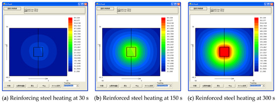
Figure 5.
Rebar temperature analysis results.
In the case of 2D analysis, it was difficult to reproduce the measurement when the temperature in the centre was high because the vortex current in the longitudinal direction of the reinforcing bar was not considered; the temperature dependence was also not considered.
However, unlike 2D analysis, it is possible to simultaneously cope with vertical and horizontal eddy currents and consider the relative permeability of reinforcing bars, so it is judged that it is possible to reproduce the curly temperature and temperature rise characteristics of reinforcing bars.
- (B)
- Results of 3D analysis
The Figure 6 shows the 3D analysis results of the reinforcement heating experiment using induction heating. To verify the correctness of the software, we analysed the induction heating of the material of the shape given in Figure 3 and compared it with the results of the experiment. The higher is the frequency, the shallower is the eddy current that is induced in the conductor. The depth at which the intensity of the electric wave on the surface shrinks to 1/e is called penetration depth (which is explained above). This phenomenon is called the skin effect, and many elements must be used for the interface with air in the analysis of electromagnetic fields considering such properties.
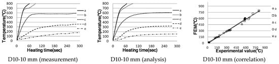
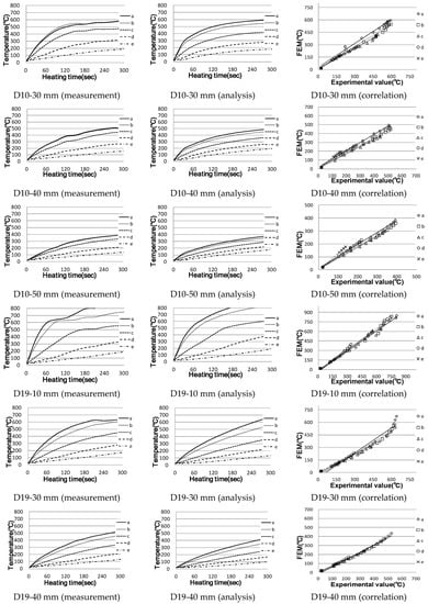
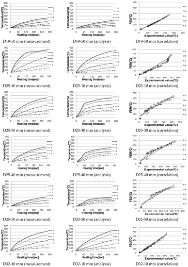
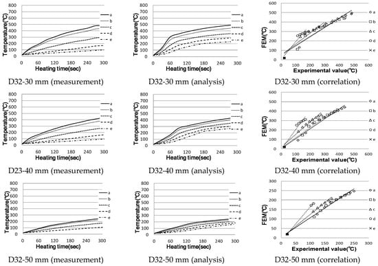
Figure 6.
Temperature rise characteristics of single rebar (correlation between actual measurement and analysis).
For the analysis of this system, it was set to power up to 300 s and then power down. As a result, the strength of the electric field is the strongest on the surface close to the induction heating coil; thus, the temperature of that part rose the most. This showed a very similar trend compared to the actual measurements but resulted in a rise in temperature. However, in the case of reinforcing bar D10, the circumscribed Point c and the horizontal axis at Point d, i.e., 30 and 60 mm away from the outer boundary of the coil, showed a slight difference compared to the measured values; however, the result was almost the same at the last temperature. It was confirmed that the difference in this tendency became smaller as the distance from the coil became smaller; however, the difference in temperature tended to increase as the distance from the centre of the reinforcing bar increased. The temperature varies rapidly depending on the heat transfer rate used in the analysis. The heat transfer rate affects the area and distance between the heated object and the heated coil; therefore, if the heat transfer rate is specified to match the distance between the reinforcing steel surface and the heated coil, the temperature difference will be greater.
In the case of D19, a temperature rise characteristic similar to the actual measurement value is shown compared to D10, and a stable result is shown even at a measurement point away from the centre of the reinforcement.
For D25 and D32, the temperature tends to be similar to the actual measurement value in the temperature rise range, but the temperature rises rapidly at the initial temperature rise rate, unlike the actual measurement value that rises while drawing a slow curve. This may be because the electric field, which is the source of induction heating, only rises from the surface to a certain depth and does not heat inside at all. In addition, heat transfer occurred inside over time, and the inside part was also heated. During the analysis, it is difficult to determine when this temperature does not rise; thus, we conclude there may be some errors in the selection at this time.
As shown in Figure 7, an eddy current is generated along the rectilinear longitude of the coil while wrapping the surface of the reinforcement.
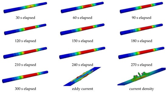
Figure 7.
Analysis results, eddy current and current density.
3.1.2. Temperature Characteristics of Cross-Bar
Figure 8 shows the comparison between the actual measurement results and the analysis results, while Figure 9 shows the shape of the eddy current and current density. For the cross-reinforcing bars, the results of D19, D25 and D32 are mostly similar, with the figures of the upper and lower D10 reinforcing bars being representative.


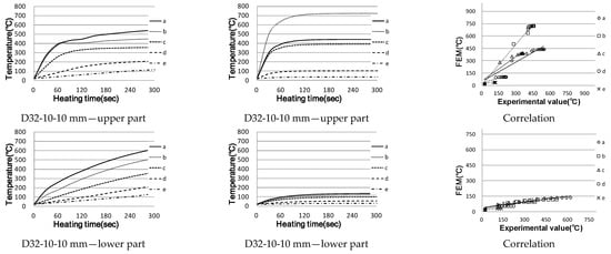
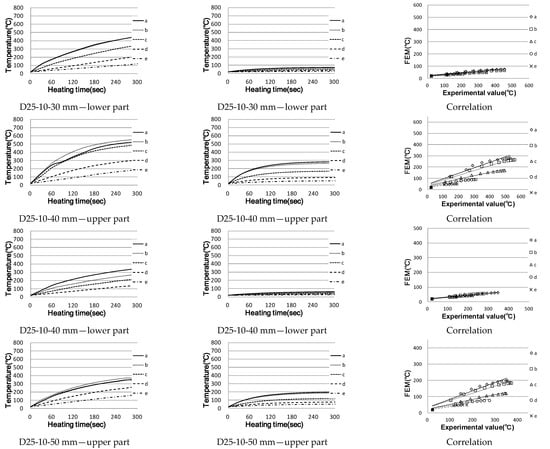
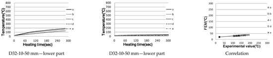
Figure 8.
Temperature rise characteristics of crossed reinforcing bar (correlation between actual measurement and analysis).
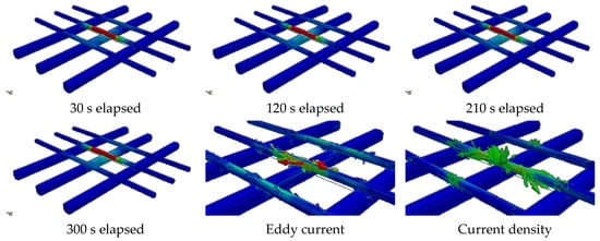
Figure 9.
Analysis results and eddy Current and current Density.
In the case of the upper reinforcing bars, the points at 10 mm away from the heating coil showed a slight temperature difference, while Points b–e showed similar results to the actual measurements. However, the results for ≥30 mm show a temperature difference smaller than the 10 mm results; however, they were still relatively close to the actual measurements.
In the case of the lower reinforcing bars, the temperature difference between the maximum measurement and the actual temperature difference of more than 550 °C was observed regardless of the distance; most of the values did not exceed 150 °C. In the case of actual reinforcing bars, an eddy current is generated mainly on the upper reinforcing bars; the lower reinforcing bars are greatly affected by heat conduction, and the temperature increases. Similarly, in the analysis of the results (in Figure 9, an eddy current is formed around D10, the upper reinforcing bar), the lower part seems to have little effect.
In addition, it can be confirmed that the current density is high around the centre of the upper reinforcing bar. Therefore, it can be determined that the temperature rise in the lower reinforcing bar is due to heat conduction from the upper reinforcing bar. However, in the case of the actual reinforcing bar, the joint is connected by a split element.
Accordingly, as much heat is taken to the lower part at the same time as the initial heat generation, the heating efficiency of the upper reinforcing steel is reduced and the amount of heat conducted by this is thought to be reduced. From now on, it is necessary to consider the lower reinforcement in the analytical part.
As mentioned above, in the case of existing crossed reinforcement models, the joint between the upper and lower reinforcing bars was made as a face joint. Unlike the actual joint of the reinforcing bars, the heat generated earlier was transferred rapidly to the lower reinforcing bars. In addition, in the case of the face joining method, the lower reinforcement was recognised as a single reinforcement, and, in the case of the lower reinforcement, an eddy current was formed in the upper reinforcement, which was rarely heated.
Therefore, in the case of the new model shown in Figure 10, thin reinforcing bars were manufactured in the form of ribs (similar to reinforcing bars) and integrated with the lower reinforcing bars to form possible point junctions. As a result, as shown in Figure 11, the eddy current is formed at the lower reinforcing bar, and the current density is also concentrated at the centre of the lower and upper reinforcing bars. The overall analysis indicates that, unlike the results of reproducing mainly existing upper reinforcing bars, upper and lower reinforcing bars were also reproduced in the same way as actual measurements.
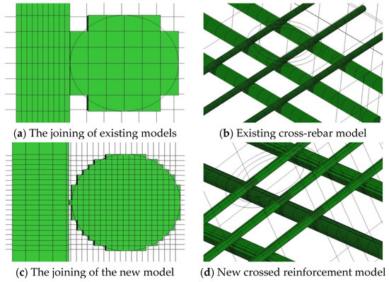
Figure 10.
3D analysis model.

Figure 11.
Analysis results, eddy current and current density.
Figure 12 show the temperature rise characteristics of crossed reinforcing bar with correlation between actual measurement and analysis. Therefore, unlike the existing model, if a steel bar that is similar to a rib is integrated into the upper part of the lower reinforcement, and the size of the rib is increased, the analysis time is slightly longer than that of the existing model, but the actual measurement is more similar.

Figure 12.
Temperature rise characteristics of crossed reinforcing bar (correlation between actual measurement and analysis).
3.2. Reinforced Concrete Temperature Characteristics Generated in Actual Environment
3.2.1. Temperature Characteristics of Single Reinforced Concrete
For single reinforced concrete, the analysis values were compared, as shown in Figure 13, assuming that the temperature measured approximately 10 mm from the surface of the actual concrete reinforcing bars using D10, D19, D25 and D32 is the same. Figure 14 shows the analysis results and the shapes of the eddy current and current density.

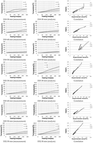

Figure 13.
Temperature rise characteristics of single reinforced concrete (correlation between actual measurement and analysis).
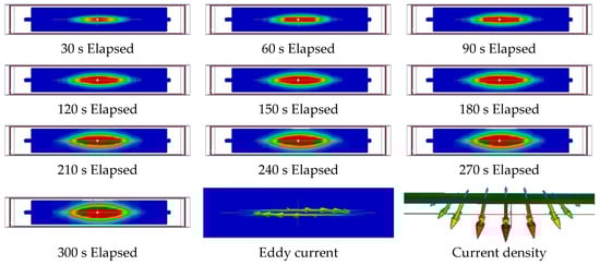
Figure 14.
Analysis results, eddy current and current density.
In the case of reinforced concrete specimens using D10 and D19 reinforcing bars, the 30 mm one with a short heating distance showed results similar to actual measurements; however, the longer is the distance, the lower is the correlation with actual measurements. However, this temperature difference is actually no very much, approximately 80 °C; it is judged that similar results to actual measurements were obtained in the temperature range that affects the vulnerability of the concrete.
The D19 and D25 reinforced concrete experiments showed the same tendency as D10, but the larger is the diameter of the reinforcing steel in the experiment, the smaller is the range of temperature difference, the thicker is the coating and the higher is the temperature. In the case of the heat transfer coefficient, it is important to study the relationship and distance between the reinforcing steel and concrete because the distance from the heated object, the area and the material are significant.
In the case of eddy currents, it is usually formed on the surface of the reinforcing steel around the rectilinear longitude of the heating coil, creating a magnetic field. Based on actual measurements, it seems that eddy currents are generated under similar conditions. In the case of current density, the closer is the skin effect to the conductor’s surface, the greater is the current density and the higher is the frequency. As shown in Figure 14, the surface of the reinforcing bar was covered in concrete; thus, the current density was almost always inside the reinforcing bar.
3.2.2. Temperature Characteristics of Cross-Reinforced Concrete
In the case of cross-reinforced concrete, the temperature rise characteristics of the actual measurement and analysis results are shown in Figure 15 (using D10 reinforcing bars as upper reinforcing bars and D19, D25 and D32 as lower reinforcing bars). Figure 16 shows the shape of the internal temperature, the shape of the eddy current and the current density over time.
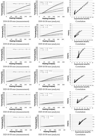
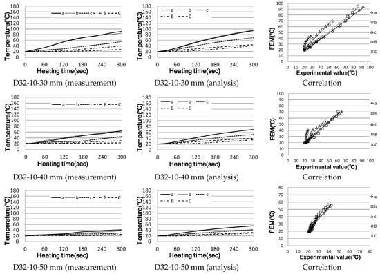
Figure 15.
Temperature rise characteristics of crossed reinforced concrete (correlation between actual measurement and analysis).

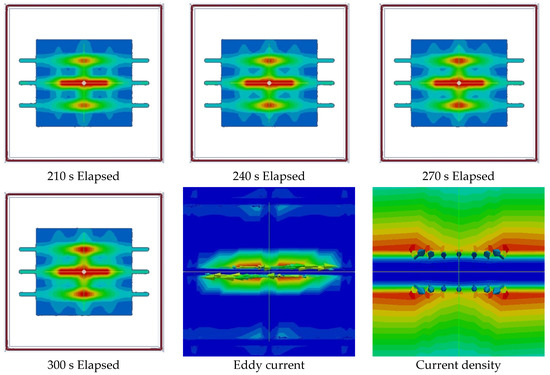
Figure 16.
Analysis results, eddy current and current density.
In the case of the cross-reinforcing bars, it was confirmed that the temperature difference between the upper D10 and centre of the upper reinforcing bar surface was approximately 30 and 60 mm. When D19 was used as a lower reinforcement, the temperature difference between the lower reinforcing bars increased in almost all experimental bodies, and the results were similar in terms of correlation. In the case of actual measurements of lower reinforcing bars, heat hardening was calculated to be low; however, in the case of the analysis values, with differences of up to 40 °C compared to actual measurements, they were calculated to be high overall.
In addition, experiments using D25 and D32 for lower reinforcing bars showed the same tendency in most cases; the temperature rise in the case of D19 was the largest in the reinforcing bar type, and the analysis showed the same result.
In the case of actual measurements, most of the eddy current is concentrated on the upper reinforcement of the intersection, whereas, in the analysis, it seems that the lower reinforcement is affected by the magnetic field. In addition, if only reinforcing bars were heated in the air, the lower reinforcing bars would be included in the magnetic field in areas close to 10 mm and the temperature would increase at the same time as the upper reinforcing bars. If the reinforcing steel is inside the concrete, the heat transferred to the lower reinforcing steel is relatively small, the heat efficiency is low, and, since the larger is the diameter of the reinforcing steel, the larger is the contact area, it is lower.
In the analysis, unlike the actual laboratory, because the reinforcing bars are in contact with each other at the surface, more heat is transferred to the lower reinforcing bar than the actual temperature. In a future analysis model, it is necessary to develop the contact shape of the joint so that it becomes a point, not a surface.
As mentioned above, a new reinforcement model was designed, and, unlike the existing model, the results of actual measurements were reproduced. Accordingly, a new reinforced concrete model was designed and analysed based on the model used for cross-reinforcement analysis. Similar to the new reinforced concrete model, a thin reinforcement similar to a rib was manufactured on the upper surface of the lower reinforcement, which was integrated and split.
As a result, similar results to the actual measurements were obtained, as shown in Figure 17. In addition, as shown in Figure 18, a vortex current was formed around the upper three reinforcing bars and only the upper reinforcing bars were heated, whereas the upper and lower reinforcing bars were heated at the same time.

Figure 17.
Temperature rise characteristics of cross-reinforced concrete (correlation between actual measurement and analysis).
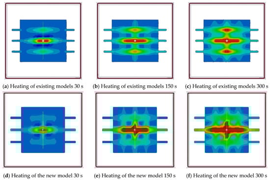
Figure 18.
Analysis results.
3.3. Actual Temperature Characteristics of Reinforced Concrete Members
3.3.1. Temperature Characteristics of Cross-Reinforced Concrete (60 mm·10 KW Cover Thickness)
Based on the results of the analysis presented in Figure 19 and Figure 20, we conducted an analysis on a 60 mm thick member that was not carried out in the experiment of this study. In this study, the temperature of the upper reinforcing bar was increased by conducting heat from the upper reinforcing bar to the lower part of the cross-reinforced concrete. In comparison with the target temperature, the temperature of the upper reinforcing bar was increased by less than 40 mm; therefore, an analysis was conducted using a reinforced concrete member with a cover thickness of 60 mm and a comparison with the results of heating the reinforcing steel using the 10 KW output conducted in a previous study.

Figure 19.
Temperature rise characteristics of crossed reinforced concrete.

Figure 20.
Analysis results.
As a result, when the 60 mm thick reinforced concrete is induction-heated using a 10 KW output, a magnetic field is generated up to the lower reinforcing bar and a resistance heating phenomenon is observed. However, the higher is the cover thickness, the lower is the temperature range, and a delay of approximately 2 min to the target temperature is observed. Therefore, if the heat of reinforced concrete increases, it is judged that it can be dealt with by increasing the power output. However, research is needed to check the area where the proper power output can be efficiently heated with no power loss using more than 10 KW.
3.3.2. Actual Part Temperature Characteristics (Beam·5 KW)
In the case of walls and slab members of structures, it is determined that they can be dealt with based on the cross-reinforced concrete in this study. However, in the case of columns and beams, different variables need to be considered depending on the reinforcement arrangement and type of reinforcement that is used. Therefore, based on the results presented in this section, an analysis model was designed and evaluated for structures (beams) that are actually used in the field (Figure 21).

Figure 21.
Summary of test sample analysis [21].
As shown in Figure 22a, the bar arrangement is the same as the bar arrangement state in Figure 21. As can be seen from the existing results, the local heating system was confirmed to have no significant effect on parts other than the heated range.

Figure 22.
Analysis model overview.
In the case of the temperature measurement site, the induction heating coil is located around the intersection of D51 and D10 reinforcing bars, as shown in Figure 23; thus, the points of 0, 30, 60 and 90 mm were measured with reference to the surface of the centre of the D51 and D19 reinforcing bars. For D10 reinforcing bars, the 0, 30, 60 and 90 mm points were measured along the D10 reinforcing bars with reference to the intersection of the vertical and horizontal parts.
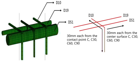
Figure 23.
Mesh and temperature measurement location details.
Based on the analysis (Figure 24) of the temperature rise characteristics of the beam member using the output of 5 KW high-frequency induction heating, it was confirmed that the temperature of the upper reinforcing bar D10 near the induction heating coil rose to the target temperature within 3 min. However, in the case of D51 reinforcing bars that came into contact with the lower part of the D10 reinforcing bars, the temperature rise characteristics were reduced. This means that the larger is the diameter of the reinforcing bar, the greater is the area of resistance to heat generation; however, it was determined that the temperature rise characteristics were reduced by heat conduction inside the reinforcing bar until it reached thermal equilibrium. In the case of D19 reinforcing bars, the heating coil is brought into contact with the outside radius of the coil, as shown in the centre of the cross-reinforced concrete specimen using existing D19 and D10 reinforcing bars.
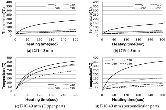
Figure 24.
Temperature rise characteristics of beam reinforced concrete.
Accordingly, it is necessary to calculate an appropriate output to increase the width of the temperature rise, owing to resistance to the heat generation compared to the internal thermal conductivity.
4. Conclusions
In this study, we analysed the thermal field generated on the surface of reinforcing steel through 2D and 3D magnetic field analyses based on previous experiments on the temperature rise characteristics of reinforcing steel, temperature rise characteristics and mechanical characteristics. According to the results of the analysis of transferred heat from heated reinforcing steel to concrete, actual reinforced concrete was analysed and compared with real measurements, and the following conclusions were reached.
First, from the 2D analysis, it is difficult to reproduce the measurements, unlike the actual measurement where the temperature in the centre is high; in addition, the temperature dependence cannot be considered, so the temperature is higher than the Curie point. Further, most of the analysis results of the single 3D reinforcement showed a tendency similar to the actual measurements. However, when the distance at the time of measurement is far from the centre or in a low-temperature region below 100 °C, a slight difference in temperature is observed compared to the actual measurement. Because the heat transfer rate used in the analysis has a significant effect on the heating distance and the diameter of the reinforcing bar, it is deemed necessary to reproduce a more accurate heat transfer rate when using deformed reinforcing bars.
Additionally, in the case of 3D analysis of crossed reinforcing bars using existing models, the reinforcing bar model was divided, and the split parts were joined in the form of faces. Similar results were found in the upper reinforcing bars, but the lower reinforcing bars showed large temperature differences. However, when the joint surface is changed to a point joint system for analysis, a result similar to the actual measurements can be obtained without changing the heat conduction or heat transfer coefficient.
In the case of the analysis of single reinforced concrete, the results are almost identical to the actual measurements. However, the 50 mm heating distance model, which shows low temperature rise characteristics, showed somewhat different results. There is a similar phenomenon for cross-reinforced concrete, but the temperature difference is within the range of 80 °C or below, and there was no significant difference in the final temperature value.
In the case of 3D analysis using the existing cross-reinforced concrete model, the analysis was conducted using the face joining model; thus, the results were slightly different from the actual measurements. However, when using the cross-reinforced concrete model that uses the point junction type, the same results were obtained when the upper and lower centre reinforcing bars were heated; then, heat was transferred to the concrete, as shown in the actual measurements of the intersection.
If the heat at the head is increased to 60 mm or more, the 10 KW output can be used to form a magnetic field in the lower reinforcing bar to induce a resistance heating phenomenon. Therefore, when the heating distance increases to 60 mm or more, it is judged that an output amount of 10 KW or more is necessary; thus, it is important to calculate the output amount in the range where there is no power loss due to the output increase.
In the case of actual members, the conditions of the reinforcement arrangement and the types of reinforcing bars used are varied, and the resistance heating characteristics are increased by the increase in the joining surface of the reinforcing bars that are in contact with the heating. Accordingly, an existing output amount of 5 KW or more is required, and the heating efficiency is determined to increase by increasing the area of the heating coil in direct contact with the reinforcing steel; thus, careful consideration of the deformation of the heating coil is required.
Author Contributions
Conceptualisation, M.-k.L.; methodology, M.-k.L.; investigation, M.-k.L.; data curation, M.-k.L.; writing—original draft preparation, C.L.; and writing—review and editing, C.L. All authors have read and agreed to the published version of the manuscript.
Funding
This work was supported by the National Research Foundation of Korea (NRF) and the grant was funded by the Korean government (NRF-2018R1D1A1B07049390).
Institutional Review Board Statement
Not applicable.
Informed Consent Statement
Not applicable.
Data Availability Statement
Not applicable.
Conflicts of Interest
The authors declare no conflict of interest.
References
- Yashiro, S.; Takatsubo, J.; Toyama, N. An NDT technique for composite structures using visualized Lamb-wave propagation. Compos. Sci. Technol. 2007, 67, 3202–3208. [Google Scholar] [CrossRef]
- Raisutis, R.; Kazys, R.; Zukauskas, E.; Mazeika, L.; Vladišauskas, A. Application of ultrasonic guided waves for non-destructive testing of defective CFRP rods with multiple delaminations. NDT E Int. 2010, 43, 416–424. [Google Scholar] [CrossRef]
- Li, P.; Xie, S.; Wang, K.; Zhao, Y.; Zhang, L.; Chen, Z.; Uchimoto, T.; Takagi, T. A novel frequency-band-selecting pulsed eddy current testing method for the detection of a certain depth range of defects. NDT E Int. 2019, 107, 102154. [Google Scholar] [CrossRef]
- Cheng, J.; Qiu, J.; Xu, X.; Ji, H.; Takagi, T.; Uchimoto, T. Research advances in eddy current testing for maintenance of carbon fiber reinforced plastic composites. Int. J. Appl. Electromagn. Mech. 2016, 51, 261–284. [Google Scholar] [CrossRef]
- Goidescu, C.; Welemane, H.; Garnier, C.; Fazzini, M.; Brault, R.; Péronnet, E.; Mistou, S. Damage investigation in CFRP com-posites using full-field measurement techniques: Combination of digital image stereo-correlation, infrared thermography and X-ray tomography. Compos. B Eng. 2013, 48, 95–105. [Google Scholar] [CrossRef]
- Xie, S.; Tian, M.; Xiao, P.; Pei, C.; Chen, Z.; Takagi, T. A hybrid nondestructive testing method of pulsed eddy current testing and electromagnetic acoustic transducer techniques for simultaneous surface and volumetric defects inspection. NDT E Int. 2017, 86, 153–163. [Google Scholar] [CrossRef]
- McCann, D.; Forde, M. Review of NDT methods in the assessment of concrete and masonry structures. NDT E Int. 2001, 34, 71–84. [Google Scholar] [CrossRef]
- Pradhan, B.; Bhattacharjee, B. Performance evaluation of rebar in chloride contaminated concrete by corrosion rate. Constr. Build. Mater. 2009, 23, 2346–2356. [Google Scholar] [CrossRef]
- Parthiban, T.; Ravi, R.; Parthiban, G. Potential monitoring system for corrosion of steel in concrete. Adv. Eng. Softw. 2006, 37, 375–381. [Google Scholar] [CrossRef]
- Pour-Ghaz, M.; Isgor, O.B.; Ghods, P. Quantitative interpretation of half-cell potential measurements in concrete 8 Advances in Civil Engineering structures. J. Mater. Civ. Eng. 2014, 21, 467–475. [Google Scholar] [CrossRef]
- Hornbostel, K.; Larsen, C.K.; Geiker, M.R. Relationship between concrete resistivity and corrosion rate—A literature review. Cem. Concr. Compos. 2013, 39, 60–72. [Google Scholar] [CrossRef]
- Takahashi, Y.; Matsubara, E.; Suzuki, S.; Okamoto, Y.; Komatsu, T.; Konishi, H.; Mizuki, J.; Waseda, Y. In-situ x-ray dif-fraction of corrosion products formed on iron surfaces. Mater. Trans. 2005, 46, 637–662. [Google Scholar] [CrossRef]
- Yeih, W.; Huang, R. Detection of the corrosion damage in reinforced concrete members by ultrasonic testing. Cem. Concr. Res. 1998, 28, 1071–1083. [Google Scholar] [CrossRef]
- Ahmed, R.; Rifat, A.A.; Yetisen, A.K.; Salem, M.S.; Yun, S.-H.; Butt, H. Optical microring resonator based corrosion sensing. RSC Adv. 2016, 6, 56127–56133. [Google Scholar] [CrossRef]
- Vrana, J.; Goldammer, M.; Bailey, K.; Rothenfusser, M.; Arnold, W.; Thompson, D.O.; Chimenti, D.E. Induction and conduction thermography: Optimizing the electromagnetic excitation towards application. AIP Conf. Proc. 2009, 1096, 518–525. [Google Scholar] [CrossRef]
- Zhang, H.; Liao, L.; Zhao, R.; Zhou, J.; Yang, M.; Zhao, Y. A new judging criterion for corrosion testing of reinforced concrete based on self-magnetic flux leakage. Int. J. Appl. Electromagn. Mech. 2017, 54, 123–130. [Google Scholar] [CrossRef]
- González, J.; Cobo, A.; González, M.; Feliu, S. On-site determination of corrosion rate in reinforced concrete structures by use of galvanostatic pulses. Corros. Sci. 2001, 43, 611–625. [Google Scholar] [CrossRef]
- Abidin, I.Z.; Tian, G.Y.; Wilson, J.; Yang, S.; Almond, D. Quantitative evaluation of angular defects by pulsed eddy current thermography. NDT E Int. 2010, 43, 537–546. [Google Scholar] [CrossRef]
- Clark, M.; McCann, D.; Forde, M. Application of infrared thermography to the non-destructive testing of concrete and masonry bridges. NDT E Int. 2003, 36, 265–275. [Google Scholar] [CrossRef]
- Clark, M.; McCann, D.; Forde, M. Infrared thermographic investigation of railway track ballast. NDT E Int. 2002, 35, 83–94. [Google Scholar] [CrossRef]
- Defer, D.; Shen, J.; Lassue, S.; Duthoit, B. Non-destructive testing of a building wall by studying natural thermal signals. Energy Build. 2002, 34, 63–69. [Google Scholar] [CrossRef]
- Engelbert, P.; Hotchkiss, R.; Kelly, W. Integrated remote sensing and geophysical techniques for locating canal seepage in Nebraska. J. Appl. Geophys. 1997, 38, 143–154. [Google Scholar] [CrossRef]
- Sakagami, T.; Kubo, S. Applications of pulse heating thermography and lock-in thermography to quantitative nonde-structive evaluations. Infrared Phys. Technol. 2002, 43, 211–218. [Google Scholar] [CrossRef]
- Baek, S.; Xue, W.; Feng, M.Q.; Kwon, S. Non-destructive corrosion detection in RC through integrated heat induction and IR thermography. J. Nondestr. Eval. 2012, 31, 181–190. [Google Scholar] [CrossRef]
- Weekes, B.; Almond, D.P.; Cawley, P.; Barden, T. Eddy-current induced thermography—Probability of detection study of small fatigue cracks in steel, titanium and nickel-based superalloy. NDT E Int. 2012, 49, 47–56. [Google Scholar] [CrossRef]
- He, Y.; Pan, M.; Tian, G.; Chen, D.; Tang, Y.; Zhang, H. Eddy current pulsed phase thermography for subsurface defect quantitatively evaluation. Appl. Phys. Lett. 2013, 103, 144108. [Google Scholar] [CrossRef]
- Liu, L.; Zheng, D.; Zhou, J.; He, J.; Xin, J.; Cao, Y. Corrosion detection of bridge reinforced concrete with induction heating and infrared thermography. Int. J. Robot. Autom. 2018, 33, 379–385. [Google Scholar] [CrossRef]
- Landau, L.D.; Lifshitz, E.M.; Pitaevskii, L.P. Electrodynamics of Continuous Media; Pergamon Press: Oxford, UK, 1960. [Google Scholar]
- Aguiar, P.M.; Jacquinot, J.-F.; Sakellariou, D. Experimental and numerical examination of eddy (Foucault) currents in rotating micro-coils: Generation of heat and its impact on sample temperature. J. Magn. Reson. 2009, 200, 6–14. [Google Scholar] [CrossRef]
- Cheng, J.; Roy, R.; Agrawal, D. Radically different effects on materials by separated microwave electric and magnetic fields. Mater. Res. Innov. 2002, 5, 170–177. [Google Scholar] [CrossRef]
- Cherradi, A.; Desgardin, G.; Provost, J.; Raveau, B. Electric & Magnetic Field Contributions to the Microwave Sintering of Ceramics Elelctroceramics IV; Wasner, R., Hoffman, S., Bonnenberg, D., Hoffmann, C., Eds.; RWTN: Aachen, Germany, 1994; Volume 2, pp. 1219–1224. [Google Scholar]
- Cao, Z.; Wang, Z.; Yoshikawa, N.; Taniguchi, S. Microwave heating origination and rapid crystallization of PZT thin films in separated H field. J. Phys. D Appl. Phys. 2008, 41, 092003. [Google Scholar] [CrossRef]
- Jin, R.; Chen, Q. Investigation of Concrete Recycling in the U.S. Construction Industry. Procedia Eng. 2015, 118, 894–901. [Google Scholar] [CrossRef]
- Chen, C.; Habert, G.; Bouzidi, Y.; Jullien, A. Environmental impact of cement production: Detail of the different processes and cement plant variability evaluation. J. Clean. Prod. 2010, 18, 478–485. [Google Scholar] [CrossRef]
- Rodríguez, G.; Del Bosque, I.F.S.; Asensio, E.; Rojas, M.I.S.D.; Medina, C. Construction and demolition waste applications and maximum daily output in Spanish recycling plants. Waste Manag. Res. 2020, 38, 423–432. [Google Scholar] [CrossRef] [PubMed]
- Xie, S.; Chen, Z.; Takagi, T.; Uchimoto, T. Quantitative non-destructive evaluation of wall thinning defect in double-layer pipe of nuclear power plants using pulsed ECT method. NDT E Int. 2015, 75, 87–95. [Google Scholar] [CrossRef]
- Matvieieva, N.; Schulze, M.; Mizukami, K.; Kharabet, I.; Heuer, H. Determination of indication depths at high frequency eddy current testing of CFRP. In Proceedings of the 10th International Symposium on NDT in Aerospace, Dresden, Germany, 24–26 October 2018; pp. 1–8. [Google Scholar]
- Mottl, Z. The quantitative relations between true and standard depth of penetration for air-cored probe coils in eddy current testing. NDT Int. 1990, 23, 11–18. [Google Scholar] [CrossRef]
- Mook, G.; Lange, R.; Koeser, O. Non-destructive characterization of carbon-fibre-reinforced plastics by means of eddy currents. Compos. Sci. Technol. 2001, 61, 865–873. [Google Scholar] [CrossRef]
- Cheng, J.; Ji, H.; Qiu, J.; Takagi, T.; Uchimoto, T.; Hu, N. Role of interlaminar interface on bulk conductivity and electrical an-isotropy of CFRP laminates measured by eddy current method. NDT E Int. 2014, 68, 1–12. [Google Scholar] [CrossRef]
- Heuer, H.; Schulze, M.; Pooch, M.; Gäbler, S.; Nocke, A.; Bardl, G.; Cherif, C.; Klein, M.; Kupke, R.; Vetter, R.; et al. Review on quality assurance along the CFRP value chain—Non-destructive testing of fabrics, preforms and CFRP by HF radio wave techniques. Compos. Part B Eng. 2015, 77, 494–501. [Google Scholar] [CrossRef]
- Schulze, M.H.; Heuer, H.; Küttner, M.; Meyendorf, N. High-resolution eddy current sensor system for quality assessment of carbon fiber materials. Microsyst. Technol. 2010, 16, 791–797. [Google Scholar] [CrossRef]
- Todoroki, A. Skin effect of alternating electric current on laminated CFRP. Adv. Compos. Mater. 2012, 21, 477–489. [Google Scholar] [CrossRef]
- Jiao, S.; Li, J.; Du, F.; Sun, L.; Zeng, Z. Characteristics of Eddy Current Distribution in Carbon Fiber Reinforced Polymer. J. Sensors 2016, 2016, 4292134. [Google Scholar] [CrossRef]
- Carpenter, C.J. Comparison of Alternative Formulations of 3-Dimensional Magnetic-Field and Eddy-Current Problems at Power Frequenies. Proc. IEE 1977, 124, 1026–1034. [Google Scholar]
- Carpenter, C. Finite-element network models and their application to eddy-current problems. Proc. Inst. Electr. Eng. 1975, 122, 455. [Google Scholar] [CrossRef]
- Chari, M.K. Finite-Element Solution of the Eddy-Current Problem in Magnetic Structures. IEEE Trans. Power Appar. Syst. 1974, PAS-93, 62–72. [Google Scholar] [CrossRef]
- Salon, S.J.; Schneider, J.M. The Application of a Finite Element Formulation of the Electric Vector Potential to Eddy Current Losses; IEEE Paper A79-545-5; IEEE: New York, NY, USA, 1979. [Google Scholar]
- Sato, T.; Sarto, S. Solution of Magnetic Field, Eddy Current and Circulating Current Problems, Taking Magnetic Saturation and Effect of Eddy Current and Circulating Current Paths into Account. In IEEE Transactions on Power Apparatus and Systems; IEEE Paper A-77-168-8; IEEE: New York, NY, USA, 1977. [Google Scholar]
- Rodger, D. Finite-element method for calculating power frequency 3-dimensional electromagnetic field distributions. IEE Proc. A Phys. Sci. Meas. Instrum. Manag. Educ. Rev. 1983, 130, 233. [Google Scholar] [CrossRef]
- Ma, Q.S.; Shao, K.R.; Li, L.R. Axisymmetric Eddy Current Field Computations by a Hybrid Finite-Series Method. IEEE Trans Magn. 1997, 33, 1338–1341. [Google Scholar] [CrossRef]


Publisher’s Note: MDPI stays neutral with regard to jurisdictional claims in published maps and institutional affiliations. |
© 2021 by the authors. Licensee MDPI, Basel, Switzerland. This article is an open access article distributed under the terms and conditions of the Creative Commons Attribution (CC BY) license (https://creativecommons.org/licenses/by/4.0/).