Socioeconomic Risks and Their Impacts on Ecological River Health in South Korea: An Application of the Analytic Hierarchy Process

Abstract

It is imperative to develop a methodology to identify river impairment sources, particularly the relative impact of socioeconomic sources, to enhance the efficiency of various river restoration schemes and policies and to have an internal diagnosis system in place. This study, therefore, aims to identify and analyze the relative importance of the socioeconomic factors affecting river ecosystem impairment in South Korea. To achieve this goal, we applied the Analytical Hierarchy Process (AHP) to evaluate expert judgement of the relative importance of different socioeconomic factors influencing river ecosystem impairment. Based on a list of socioeconomic factors influencing stream health, an AHP questionnaire was prepared and administered to experts in aquatic ecology. Our analysis reveals that secondary industries form the most significant source of stream ecosystem impairment. Moreover, the most critical socioeconomic factors affecting stream impairment are direct inflow pollution, policy implementation, and industrial wastewater. The results also suggest that the AHP is a rapid and robust approach to assessing the relative importance of different socioeconomic factors that affect river ecosystem health. The results can be used to assist decision makers in focusing on actions to improve river ecosystem health.

1. Introduction

Socioeconomic events such as urbanization, industrialization, and agriculture can have mixed impacts on stream environments, including various negative effects [1]; these events can be sources of major impairments to stream ecosystems [2]. Uncovering the sources of impairment is a particularly important task for the sustainable management of river ecosystems.

The Causal Analysis and Diagnosis Decision Information System (CADDIS) [3] and Eco Evidence [4] are used internationally to assess the status of stream ecosystem impairment. Although they do not focus on the causal pathway in their assessments, they have identified various socioeconomic factors—namely, land use, population, and industry—as critical sources of impairment. Moreover, the Conservation Measures Partnership (CMP) provides the Open Standards for conservation projects [5]. Within the standards, socioeconomic factors are considered indirect threats. Particularly, the standards include a step to understand the various elements related to a conservation project, such as social, economic, and political factors, in order to establish conservation goals. In a situation model for watershed site conservation projects, socioeconomic factors such as population growth, urbanization, and policy are reflected as factors influencing the direct threat.

Accordingly, socioeconomic causes must be taken into account in addition to the physical, chemical, and biological stream impairment factors, to achieve sustainable stream restoration. Some researchers have focused on such socioeconomic factors, identifying land use and land cover (LULC), impermeable paving, population density, main industries, mining, and policies relating to the stream [6,7,8,9,10,11,12,13,14,15,16,17] as impairment causes. In particular, a number of studies investigate LULC as a source of stream impairment. The land use and ground coverage in the watershed area act as nonpoint pollution sources and negatively impact the stream ecosystem [18]. Similarly, urbanization has been found to negatively impact stream ecosystems [19,20,21]. Human settlement activities in the watershed generate pollution from land development, such as infrastructure construction as well as pollution caused by living sewage. Yang et al. [22] conducted a study to understand the functional relationship between river networks and the distribution of wastewater treatment plants (WWTP), human populations (POP), and population equivalents (PE).

Stream ecosystem changes caused by economic activities can be divided into three industrial types, namely: primary, secondary, and tertiary industries. The primary industry includes agriculture, fishery, and farming; many studies have been conducted on the impact of the primary industry on river system impairment. Primary industries undermine river ecosystems, and agriculture in the watershed inevitably destroys or modifies ecosystems; a notable example is the expansion of arable land and related deterioration of water quality due to the inflow of irrigation water. Indeed, economic and agricultural activities in a riparian buffer zone have been shown to have a significant negative impact on stream ecosystems [23,24]. In addition, arable land near rivers can cause river pollution through the use of chemicals such as soil modifiers, fertilizers, and pesticides. Similarly, fisheries can contaminate river ecosystems through aquaculture facilities and feed; furthermore, reckless fishing activities change river ecosystems. The livestock industry is also detrimental to river ecosystems as manure and livestock wastewater impede water from entering the ground due to increased soil pressure, resulting in reduced ground permeability.

Studies have also been carried out on the impact of secondary industries such as mining [25,26,27,28,29]. Mining fields affect not only the adjacent soil but also the toxicity levels in streams and are thus a direct, strong negative source of stream impairment; moreover, they have been found to change the chemical characteristics of stream sediments [24,30]. According to a study carried out by Liu et al. [31], the water demand increases in the manufacturing and service industries as a result of population increases have resulted in water shortage and containment.

To date, studies focusing on the socioeconomic impacts of stream impairment have identified various human aspects of LULC, primary/secondary/tertiary industries, and policies. The identification of the relative importance of the different socioeconomic factors of stream impairment could assist in prioritizing processes during ecological stream restoration and, consequently, support related policymaking. However, the identification of stream ecosystem impairment sources is complex and challenging as it involves understanding the socioeconomic factors affecting stream ecosystem impairment and interpreting these issues.

Moreover, until now, physical and chemical factors have been the main foci in studies of stream management and restoration; in particular, in South Korea, task forces for ecological stream restoration are largely established based on physical and chemical evaluation. However, a holistic method that includes environmental, social, and economic dimensions is required to improve watershed management [1,32,33]. The application of such a holistic approach to management is currently hindered by the separate evaluations of the social, environmental, and other factors influencing stream ecosystem health [1,34,35]. Particularly, many studies on the socioeconomic factors of stream impairment have been case studies, and there is a lack of research on how we may best prioritize individual impairment factors in order to make policy decisions. This lack of information makes it difficult to conduct a universal assessment of the fundamental socioeconomic factors impairing stream health [1]. Hence, it is necessary to grasp the relative importance of different socioeconomic factors.

2. Research Methodology

This study aims to explore the socioeconomic factors affecting river ecosystems and to compare and analyze their importance. To analyze the relative importance of various socioeconomic factors, complex decision making by experts from a related field is required. Therefore, Multi-Criteria Decision Analysis (MCDA), which is a scientific discipline related to the operational research method, could be employed to analyze expert judgements. There are various MCDA methods, including the Technique for Order of Preference by Similarity to Ideal Solution (TOPSIS), VlseKriterijumska Optimizacija I Kompromisno Resenje (VIKOR), Complex Proportional Assessment (COPRAS), and Analytic Hierarchy Process (AHP) [36,37,38]. In particular, the AHP method is known to reflect the multi-layer structures of the decision-making process and is often used to analyze unpredictable situations and for multiple evaluation standards [39,40].

In recent research with industrial cases [41], weighted values were extracted using AHP methods for efficient environmental decision making. Pawlewicz et al. [42] employed AHP to understand and evaluate a regional development process with environmental, social, and economic aspects. Hence, prioritizing such elements may inform regional development evaluation and policy. AHP analysis can play an important role in supporting complicated decision-making processes. Recently, moreover, there are several studies on developments of hybrid AHP models, such as AHP-TOPSIS and AHP-MAUT, to improve the AHP [43]. The AHP not only creates a promising opportunity to deliver an efficient analytical process but also considers the experiences of experts and decision makers. Therefore, this study attempted to derive the socioeconomic factors affecting ecological river health and to compare their importance by applying the AHP method, which enables the appropriate evaluation of expert judgements.

The AHP analysis included qualitative and quantitative evaluations of various dimensions and categories and was conducted by experts. In general, AHP analysis consists of four steps: (1) goal setting and judgment criteria; (2) evaluation; (3) consistency verification; and (4) deriving weight [40,44].

First, a review was performed of the literature on stream ecosystem impairment and evaluation methods to identify the socioeconomic factors causing stream impairment. From this review, frequently emerging factors that cause stream ecosystem impairment were identified. Following an internal discussion and interviews with experts, based on verifiability and evaluation use, 6 main groups and 21 detailed factors were listed for verification. Then the main and detailed socioeconomic factors were listed as quantitative values, as shown in Figure 1. The socioeconomic factors of stream ecosystem impairment were divided into six main categories: population; policy and facility; primary, secondary, and tertiary industries; and urbanization. Population estimates the effects of the density and fluctuation of the population within the watershed area. The policy and facilities category determines the effects of the national policy, non-governmental organization (NGO) activities such as regional government budgets, the cleaning capacity, and NGO funding resources. The primary industries category includes agriculture, fishery, and livestock farming; furthermore, to produce a detailed analysis, the rice field area, the field area, the scale of farm, and the number of livestock are measured. The secondary industries category includes the mining area’s coverage, the size of aggregate extraction area, the scale of power production facilities, and the scale of the industrial complex. The numbers of water sports users, visitors at local fairs, accommodation facilities, and restaurants are included in the tertiary industries category. The urbanization category includes the commercial, residential, road, and green area ratios.

The AHP method was then applied to determine the hierarchical relative importance of the items. As part of the analysis, the AHP structure containing 6 main and 21 detailed categories was first generated. The categories and subcategories were evaluated and analyzed through paired comparison bridges. If there are n judgment criteria, the total number of evaluations is n (n − 1)/2 times. For example, 6 criteria were set in this study, and the total number of evaluation criteria was 15. The assessment criteria in AHP are composed with a pairwise comparison matrix (a square matrix of size n × n), and the technical and normative models coexist in its interpretation [40,45]. The pairwise comparisons may be represented as follows:

$$\begin{gathered} \begin{array}{ccccc}{a}_1& a_2& \dots & \dots & a_n\end{array} \\ A=\begin{array}{c}{a}_1\\ a_2\\ \dots \\ \dots \\ a_n\end{array}\left[\begin{array}{ccccc}1& a_{12}& a_{13}& \dots & a_{1n}\\ a_{21}& 1& a_{23}& \dots & a_{2n}\\ a_{31}& a_{32}& 1& \dots & a_{3n}\\ \dots & \dots & \dots & \dots & \dots \\ a_{n1}& a_{n2}& a_{n3}& \dots & 1\end{array}\right] \end{gathered}$$

(1)

MATRIX A is the inverse centered on the diagonal (i.e., a_ij = 1/a_ji and a_ii = 1), where a₁₂ indicates how much more important a₁ is compared to a₂. This evaluation process is applied in the same way to each detailed criterion. A total of 43 pairwise comparison items were evaluated. Furthermore, in the AHP analysis, the relative importance evaluation usually uses a nine-point verbal scale on the basis of social psychology. The meaning of each measure is shown in

Table 1. The fundamental scale.

Intensity of Importance	Definition	Explanation
1	Equal importance	Two activities contribute equally to the objective
2	Weak
3	Moderate importance	Experience and judgment slightly favor one activity over another
4	Moderate plus
5	Strong importance	Experience and judgment strongly favor one activity over another
6	Strong plus
7	Very strong or demonstrated importance	An activity is favored very strongly over another; its dominance is demonstrated in practice
8	Very, very strong
9	Extreme importance	The evidence favoring one activity over another is of the highest possible order of affirmation

.

Consistency verification was performed on the collected data to confirm their validity by checking for high logical consistency. One of the strengths of AHP is the provision of a mechanism for reviewing the applicator’s consistency, which eliminates the transitivity contradiction of evaluator judgment [44]. CR (Consistency Ratio) is used to measure response consistency. Although it depends on the complexity of the hierarchical structure, a CR of 0.1 or less is generally judged as consistent [45]. If the CR is between 0.1 and 0.2, it is considered acceptable and if it is above 0.2, the consistency issue must be reviewed [46]. After the consistency review, the final result was derived from the pairwise comparison of the alternatives, and the importance of each alternative was determined by calculating the eigenvalue of mathematics from the pairwise comparison matrix. The sum of the final weighted value of impairment source by respondent was calculated by geometric means and an AHP analysis was performed.

The data were collected over approximately two weeks, between 17 November 2015 and 3 December 2015. The interviewees, that is, experts in the fields of stream ecosystem, landscape restoration, and watershed management, were contacted by telephone and, after providing verbal consent, the weblinks of the questionnaires were emailed to 86 experts. A total of 59 completed questionnaires were received.

3. Results and Discussion

3.1. Respondent Profile and Sample Size

Through a pairwise comparison, only 35 respondents for whom the consistency ratio (CR) was below 0.2 were chosen as a valid sample. The remaining responses were omitted from further evaluations due to inconsistencies as reflected by their CR values.

Table 2. Respondent profile and sample size for AHP analysis.

Division		Sample Size (N)	Percentage
Total		35	100.0
Gender	Male	32	91.4
	Female	3	8.6
Age	30s	7	20.0
	40s	17	48.6
	50s	11	31.4
Affiliation	Public enterprise	6	17.1
	National research center	2	5.7
	University	14	40.0
	Private business	13	37.1
Subject	Aquatic ecology	16	45.7
	Landscape architecture	13	37.1
	Water resources	4	11.4
	Other	2	5.7
Experience (Years)	<10	10	28.6
	11–20	13	37.1
	21–30	12	34.3
Public service	Yes	32	91.4
	No	3	8.6

presents the respondent data [47].

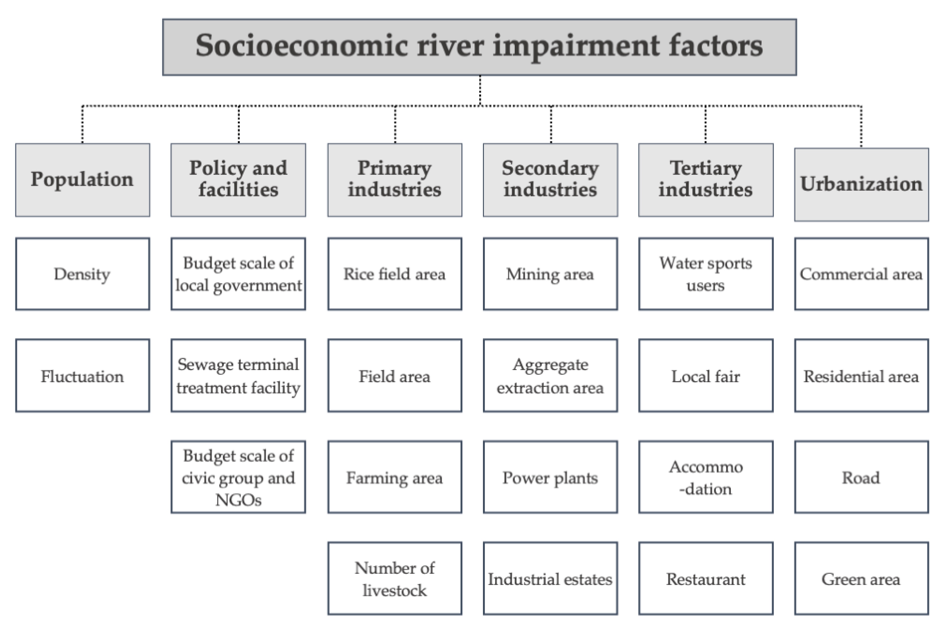
3.2. Weight Value Analysis of Socioeconomic Factors Affecting River Impairment

Among the six categories that affect the ecological river health, secondary industries (0.200), such as mines, aggregate extraction, power plants, and industrial complexes, and policy and facilities (0.199), such as budgets of local governments and civic groups, and sewage treatment facilities, were weighted relatively high compared to other categories. Primary industries, such as rice fields, fields, farms, and livestock, in the watershed had a weight of 0.172, urbanization was weighted 0.156, and tertiary industry 0.146.

By contrast, population, such as population density and population fluctuation in the watershed, was weighted at 0.127, making it a comparatively less important factor. In terms of the age of the experts, those in their thirties weighed policy and facilities higher (0.301), and those in their forties emphasized the importance of the secondary industry (0.230). No significant differences in the weights of all categories, including the level of urbanization, were detected for those in their fifties. In terms of major fields, aquatic ecological experts weighted the secondary industry relatively high (0.198), with little variation across other categories. By contrast, landscape experts placed policy and facilities (0.247) above all other factors (

Table 3. Weight value analysis of categories of socioeconomic factors.

Division		N	Population	Policy and Facilities	Primary Industries	Secondary Industries	Tertiary Industries	Urbanization
Total		35	0.127	0.199	0.172	0.200	0.146	0.156
Gender	Male	32	0.130	0.206	0.168	0.197	0.144	0.155
	Female	3	0.094	0.135	0.213	0.229	0.168	0.162
Age	30s	7	0.115	0.301	0.166	0.166	0.123	0.129
	40s	17	0.118	0.184	0.188	0.230	0.134	0.145
	50s	11	0.144	0.166	0.148	0.175	0.178	0.189
Affiliation	Public enterprise	6	0.123	0.245	0.110	0.192	0.146	0.184
	National research center	2	0.080	0.291	0.083	0.099	0.200	0.248
	University	14	0.123	0.191	0.200	0.162	0.165	0.159
	Private business	13	0.134	0.167	0.190	0.269	0.115	0.124
Subject	Aquatic ecology	16	0.160	0.171	0.162	0.198	0.151	0.158
	Landscape architecture	13	0.110	0.247	0.147	0.187	0.134	0.174
	Water resources	4	0.086	0.177	0.345	0.202	0.111	0.078
	Other	2	0.075	0.140	0.135	0.228	0.235	0.187
Experience (Years)	<10	10	0.119	0.262	0.146	0.150	0.156	0.167
	11–20	13	0.101	0.216	0.165	0.226	0.135	0.157
	21–30	12	0.163	0.139	0.198	0.214	0.145	0.141
Public service	Yes	32	0.129	0.203	0.156	0.199	0.148	0.164
	No	3	0.087	0.135	0.415	0.178	0.108	0.077

).

3.2.1. Population

The subcategories related to population that affect river health are population density and fluctuation in the watershed (

Table 4. Weight value analysis of subcategories of socioeconomic factors—Population.

Division		N	Density	Fluctuation
Total		35	0.638	0.362
Gender	Male	32	0.624	0.376
	Female	3	0.766	0.234
Age	30s	7	0.566	0.434
	40s	17	0.689	0.311
	50s	11	0.599	0.401
Affiliation	Public enterprise	6	0.405	0.595
	National research center	2	0.528	0.472
	University	14	0.665	0.335
	Private business	13	0.721	0.279
Subject	Aquatic ecology	16	0.656	0.344
	Landscape architecture	13	0.568	0.432
	Water resources	4	0.771	0.229
	Other	2	0.634	0.366
Experience (Years)	<10	10	0.532	0.468
	11–20	13	0.625	0.375
	21–30	12	0.730	0.270
Public service	Yes	32	0.638	0.362
	No	3	0.636	0.364

). Overall, the experts who participated in the survey determined that population density (0.638) was more important than population fluctuation (0.362). However, experts employed in public enterprises rated population fluctuation (0.595) as more important than population density (0.405).

3.2.2. Policy and Facilities

The subcategories related to policy and facilities affecting damage to river ecosystems are budget scale of local streams, sewage terminal treatment facility, and budget scale of civic groups and NGOs (

Table 5. Weight value analysis of subcategories of socioeconomic factors—Policy and facilities.

Division		N	Budget Scale of Local Streams	Sewage Terminal Treatment Facility	Budget Scale of Civic Groups and NGOs
Total		35	0.387	0.500	0.113
Gender	Male	32	0.394	0.491	0.115
	Female	3	0.314	0.600	0.086
Age	30s	7	0.398	0.509	0.094
	40s	17	0.374	0.507	0.118
	50s	11	0.399	0.483	0.118
Affiliation	Public enterprise	6	0.481	0.416	0.104
	National research center	2	0.277	0.633	0.089
	University	14	0.385	0.475	0.139
	Private business	13	0.362	0.543	0.095
Subject	Aquatic ecology	16	0.371	0.498	0.131
	Landscape architecture	13	0.467	0.440	0.093
	Water resources	4	0.317	0.605	0.078
	Other	2	0.185	0.632	0.183
Experience (Years)	<10	10	0.390	0.478	0.132
	11–20	13	0.378	0.511	0.111
	21–30	12	0.394	0.506	0.100
Public service	Yes	32	0.379	0.506	0.115
	No	3	0.471	0.439	0.090

). The sewage terminal treatment facility factor was rated the highest, with a value of 0.500. The budget scale of local streams was weighted as 0.387, and the budget scale of civic groups and NGOs was weighted as 0.113, which was relatively insignificant. Most experts rated the importance of the sewage terminal treatment facility the highest. Experts affiliated to public enterprises believed that the budget scale of local streams (0.481) was more important than the sewage terminal treatment facility (0.416). Landscape architecture experts rated the budget scale of local streams (0.467) as more important than the sewage terminal treatment facility (0.440).

3.2.3. Primary Industries

The subcategories related to primary industries affecting ecological river health include rice field area, field area, aquaculture area, and number of livestock (

Table 6. Weight value analysis of subcategories of socioeconomic factors—Primary industries.

Division		N	Rice Field Area	Field Area	Aquaculture Area	Number of Livestock
Total		35	0.129	0.142	0.221	0.508
Gender	Male	32	0.130	0.134	0.219	0.517
	Female	3	0.117	0.253	0.235	0.395
Age	30s	7	0.141	0.198	0.255	0.406
	40s	17	0.125	0.133	0.202	0.540
	50s	11	0.127	0.123	0.229	0.521
Affiliation	Public enterprise	6	0.136	0.116	0.266	0.482
	National research center	2	0.185	0.344	0.158	0.313
	University	14	0.117	0.114	0.261	0.509
	Private business	13	0.128	0.164	0.172	0.536
Subject	Aquatic ecology	16	0.131	0.212	0.180	0.477
	Landscape architecture	13	0.141	0.097	0.239	0.523
	Water resources	4	0.097	0.098	0.299	0.506
	Other	2	0.090	0.100	0.293	0.517
Experience (Years)	<10	10	0.113	0.143	0.287	0.457
	11–20	13	0.130	0.155	0.180	0.534
	21–30	12	0.141	0.125	0.219	0.514
Public service	Yes	32	0.126	0.146	0.210	0.517
	No	3	0.153	0.096	0.363	0.388

). The weight analysis showed that the number of livestock in the watershed has the highest impact on river ecosystem degradation (0.508). The aquaculture area had a weight of 0.221, the field area 0.142, and the rice field area 0.129, indicating these factors are less important than the number of the livestock in the watershed. Most experts weighted the number of livestock the highest. This is because livestock feces and wastewater, which are likely to leak directly from farms into rivers, are perceived to have a more significant impact on the river ecosystem compared to agriculture or aquaculture problems.

3.2.4. Secondary Industries

The subcategories of secondary industries include mining area, aggregate extraction, power plants, and industrial estates (

Table 7. Weight value analysis of subcategories of socioeconomic factors—Secondary industries.

Division		N	Mining Area	Aggregate Extraction	Power Plants	Industrial Estates
Total		35	0.215	0.262	0.145	0.378
Gender	Male	32	0.207	0.251	0.142	0.400
	Female	3	0.281	0.370	0.167	0.183
Age	30s	7	0.263	0.215	0.137	0.385
	40s	17	0.198	0.280	0.155	0.367
	50s	11	0.213	0.266	0.136	0.386
Affiliation	Public enterprise	6	0.303	0.197	0.146	0.354
	National research center	2	0.199	0.364	0.118	0.320
	University	14	0.211	0.243	0.165	0.381
	Private business	13	0.185	0.300	0.127	0.387
Subject	Aquatic ecology	16	0.191	0.300	0.141	0.369
	Landscape architecture	13	0.239	0.183	0.142	0.436
	Water resources	4	0.192	0.421	0.115	0.273
	Other	2	0.250	0.250	0.250	0.250
Experience (Years)	<10	10	0.278	0.213	0.156	0.354
	11–20	13	0.155	0.285	0.119	0.440
	21–30	12	0.238	0.273	0.163	0.326
Public service	Yes	32	0.208	0.254	0.145	0.393
	No	3	0.284	0.337	0.145	0.234

). The weights were as follows: industrial estates (0.378), aggregate extraction (0.262), mining area (0.215), and power plants (0.145). Most experts across all demographics thought that the area ratio of industrial estates was the most important factor. This can be interpreted as reflecting their concerns about the pollutants generated in industrial complexes. Opinions, however, were divided regarding the second-highest ranking socioeconomic factor affecting river ecosystems. Aquatic ecologists rated aggregate extraction area (0.300) as more important than mining area (0.191). By contrast, landscape experts found the mining area ratio (0.239) as more important than the aggregate extraction area (0.183).

3.2.5. Tertiary Industries

The subcategories of tertiary industries affecting ecological river health were water sports users, local fairs, accommodations, and restaurants (

Table 8. Weight value analysis of subcategories of socioeconomic factors—Tertiary industries.

Division		N	Water Sports Users	Local Fair	Accommodation	Restaurant
Total		35	0.161	0.170	0.260	0.409
Gender	Male	32	0.157	0.171	0.254	0.419
	Female	3	0.199	0.157	0.335	0.308
Age	30s	7	0.173	0.179	0.261	0.387
	40s	17	0.143	0.163	0.265	0.430
	50s	11	0.184	0.174	0.252	0.390
Affiliation	Public enterprise	6	0.219	0.227	0.222	0.332
	National research center	2	0.073	0.153	0.291	0.484
	University	14	0.180	0.173	0.251	0.396
	Private business	13	0.136	0.144	0.278	0.442
Subject	Aquatic ecology	16	0.170	0.152	0.274	0.404
	Landscape architecture	13	0.143	0.198	0.236	0.423
	Water resources	4	0.154	0.128	0.271	0.447
	Other	2	0.221	0.240	0.270	0.270
Experience (Years)	<10	10	0.187	0.205	0.251	0.357
	11–20	13	0.118	0.142	0.255	0.485
	21–30	12	0.192	0.171	0.267	0.370
Public service	Yes	32	0.154	0.167	0.261	0.418
	No	3	0.247	0.199	0.244	0.310

). Experts who participated in the survey believed that the number of restaurants (0.409) had the greatest impact on the damage to the river ecosystem, while the importance of the number of accommodations (0.260) was also relatively high. By contrast, the importance of local fairs (0.170) and water sports users (0.161) was relatively low. Across expert demographics, the weight of the number of restaurants was highest, and that of the number of accommodations was second highest. These trends affirm the greater concern regarding pollutants that can directly enter the stream, rather than indirect pollutants from water sports facilities or local fairs.

3.2.6. Urbanization

Among the factors affecting river health, subcategories for urbanization are commercial, residential, road, and green areas (

Table 9. Weight value analysis of subcategories of socioeconomic factors—Urbanization.

Division		N	Commercial Area	Residential Area	Road Area	Green Area
Total		35	0.430	0.241	0.211	0.119
Gender	Male	32	0.431	0.254	0.210	0.105
	Female	3	0.341	0.111	0.181	0.366
Age	30s	7	0.391	0.234	0.204	0.172
	40s	17	0.444	0.209	0.210	0.137
	50s	11	0.421	0.296	0.209	0.073
Affiliation	Public enterprise	6	0.440	0.233	0.227	0.100
	National research center	2	0.449	0.189	0.192	0.170
	University	14	0.380	0.256	0.232	0.132
	Private business	13	0.476	0.234	0.183	0.107
Subject	Aquatic ecology	16	0.415	0.230	0.234	0.121
	Landscape architecture	13	0.475	0.220	0.198	0.108
	Water resources	4	0.315	0.372	0.154	0.159
	Other	2	0.465	0.225	0.219	0.091
Experience (Years)	<10	10	0.408	0.225	0.222	0.145
	11–20	13	0.460	0.259	0.188	0.093
	21–30	12	0.412	0.233	0.225	0.130
Public service	Yes	32	0.443	0.233	0.212	0.112
	No	3	0.290	0.324	0.179	0.207

). In terms of the weight analysis, the importance of commercial area was the highest, at 0.430, followed by residential area (0.241), roads (0.211), and green areas (0.119). Most experts judged the commercial area as most important, while aquatic ecologists indicated that the residential area (0.372) was more important than the commercial area (0.315).

3.2.7. Overall Weights

As presented in

Table 10. Overall weight and rankings of subcategories of socioeconomic stream impairment sources.

Subcategory	Overall Weight	Overall Rankings
Sewage terminal treatment facility	0.099	1
Number of livestock	0.087	2
Population density	0.081	3
Budget scale of local streams	0.077	4
Industrial estates	0.076	5
Commercial area	0.067	6
Restaurant	0.060	7
Aggregate extraction area	0.052	8
Population fluctuation	0.046	9
Mining area	0.043	10
Farming area	0.038	11
Accommodation	0.038	11
Residential area	0.038	11
Road	0.033	14
Power plants	0.029	15
Local fair	0.025	16
Field area	0.024	17
Water sports users	0.024	17
Budget scale of civic groups and NGOs	0.022	19
Rice field area	0.022	19
Green area	0.019	21

, the study next analyzed the weighted hierarchal values of the 21 detailed criteria of the socioeconomic sources of stream ecosystem impairment. After combining the weights of the six criteria used in this analysis and the weights of each of the subcategories, the most important factor affecting the damage to the river ecosystem was the sewage terminal treatment facility (0.099). This was followed by number of livestock (0.087), population density (0.081), budget scale of local streams (0.077), industrial estates (0.076), commercial area (0.067), number of restaurants (0.060), and aggregate extraction area (0.052). The weight of these factors stands out among the 21 different factors, reflecting the experts’ concerns about pollutants likely to flow directly into the river [47]. Considering this together with the importance of local budgets, the result can also be interpreted as emphasizing the need for active and proactive policies to preserve river ecosystems.

In the AHP results of all six categories, the secondary industries and policy and facilities categories were evaluated to be relatively important factors. The analysis illustrated relatively consistent responses among most groups of experts. In terms of major fields, however, the aquatic ecological experts weighted secondary industry relatively high; meanwhile, the landscape experts group evaluated policy and facilities as the most important factor.

Moreover, several features were identified after extensive analysis of the top 10 items from among the 21 subcategories. As shown in Figure 2 below (three dashed line boxes), three critical factors of stream impairment can be derived: direct inflow pollution, policy implementation, and industrial wastewater.

There are several causes of the critical factors identified above (direct inflow pollution, policy implementation, and industrial wastewater). First, the highest ranked causes were sewage terminal treatment facility, number of livestock, and population density; these causes were evaluated as direct inflow pollution sources by most experts. Increases in population density create organic contaminant discharge, such as human sewage, food waste, and industrial wastes, which also cause increases in chemical oxygen demand (COD) concentration [48,49,50,51]. The number of livestock also escalates total nitrogen (TN), total phosphorus (TP), biochemical oxygen demand (BOD), and so on. This effect contributes to stream ecosystem impairments. Therefore, the experts claimed that the sewage terminal treatment facility is important since it could stop the direct inflow of pollution sources. Simultaneously, they recognized local budgets as a critical factor since policy and budgets play a key role in stream ecosystems. Moreover, socioeconomic factors related to the secondary industries need to be dealt with seriously as sources of stream impairment. These sources generate industrial wastewater, which includes heavy metals [28,29]. Byrne et al. [28] suggested that an interdisciplinary approach is required for the effective restoration of mining-impacted river systems.

The socioeconomic factors affecting stream ecosystems are highly complicated; therefore, they must be dealt with comprehensively in order to adequately address multiple-stressor situations. However, the existing literature tends to separately explore these socioeconomic factors. In fact, these issues have been typically studied through case studies. These scholarly trends contribute to difficulties understanding the inter-related and multiple-stress situations impacting stream conservation and restoration [52,53]. Therefore, this study provides critical information for comprehensively addressing socioeconomic factors in stream management and restoration.

4. Conclusions

Previous evaluations and analyses of river ecosystem impairment have tended to focus on chemical and physical approaches. The ways in which socioeconomic factors serve as fundamental sources of impairment and their relative importance have been neglected, especially in South Korea. To develop a holistic methodology, not only does a physical, chemical, and biological evaluation need to be carried out, but the social and economic impairment sources also must be identified.

In this case, we evaluated 21 socioeconomic river impairment factors, which we also grouped into 6 larger categories. Among the six categories of socioeconomic factors that affect ecological river health, secondary industries and policy and facilities were weighted relatively high, followed by primary industries, urbanization, tertiary industry, and population. The overall weights presented here suggest that the presence of a sewage terminal treatment facility, the number of livestock, population density, the budget scale of local streams, and industrial estates were the most influential factors determining stream impairment. The study results can guide a holistic approach to the issue by determining the relative importance of the socioeconomic factors impacting stream ecosystem health, and in doing so, responding to the gap in existing literature, which tends to deal with these factors individually. In particular, in presenting this understanding of complicated real stream issues and the factors of stream ecosystem health, the study results could inform future decision-making processes related to stream management and restoration.

Additionally, we showed that the AHP method is a quick and robust approach to evaluating the relative degree of importance of different socioeconomic factors affecting river impairment. The AHP method evaluates the consistency of answers from each subject expert and enables the selection of consistent responses for analyses. The AHP method is flexible in terms of content and can be applied to any ecosystem evaluation. The approach allows pathways of sources of impairment to levels of impairment to be understood without quantitative modeling of the ecosystem, which requires significant data and analytical expertise. It provides a pragmatic way of assessing the most critical factors in ecosystem restoration and can thus guide decision makers regarding which factors they should target for effective and efficient restoration. This approach requires identifying and organizing factors that affect the criteria being evaluated.

However, the study suffers from the limitation that the number of expert respondents was relatively small, thus leading to a narrow range of reflection from different fields. Besides, some critics point to the “rank reversal” problem in MCDA methodology, including AHP [54]. This is a phenomenon in which an existing rank change occurs when a new factor is added or an existing factor is removed [36,54]. Hence, in future research, it is necessary to consider the rank reversal problem. The current study leaves an opportunity to identify the hierarchal differences in various fields by expanding the spectrum of expertise in further research. AHP questionnaires should be expanded and repeatedly administered to generate credible analysis and results. In addition, the positive and negative factors within the socioeconomic stream impairment sources need to be differentiated in order to draw in-depth and precise hierarchal weighted values.

References

1. Sanchez, G.M.; Nejadhashemi, A.P.; Zhang, Z.; Marquart-Pyatt, S.; Habron, G.; Shortridge, A. Linking Watershed-Scale Stream Health and Socioeconomic Indicators with Spatial Clustering and Structural Equation Modeling. Environ. Model. Softw. 2015, 70, 113–127. [Google Scholar] [CrossRef]
2. Kang, B.; Son, J. The Study on the Evaluation of Environment Function at Small Stream -In the Case of Hongdong Stream in Hongsung-Gun-. J. Korea Soc. Environ. Restor. Technol. 2011, 14, 81–101. [Google Scholar]
3. EPA. The Causal Analysis/Diagnosis Decision Information System (CADDIS); EPA: Washington, DC, USA, 2017. [Google Scholar]
4. Nichols, S.; Webb, A.; Stewardson, M. Eco Evidence Analysis Methods Manual: A Systematic Approach to Evaluate Causality in Environmental Science; eWater CooperativeResearch Centre: Canberra, Australia, 2011. [Google Scholar]
5. Stewart, A. Conservation Standards 4.0 Revisions Committee. Available online: https://conservationstandards.org/wp-content/uploads/sites/3/2020/10/CMP-Open-Standards-for-the-Practice-of-Conservation-v4.0.pdf (accessed on 18 February 2021).
6. Ge, Y.; Dou, W.; Gu, Z.; Qian, X.; Wang, J.; Xu, W.; Shi, P.; Ming, X.; Zhou, X.; Chen, Y. Assessment of Social Vulnerability to Natural Hazards in the Yangtze River Delta, China. Stoch Environ. Res Risk Assess. 2013, 27, 1899–1908. [Google Scholar] [CrossRef]
7. Tate, E. Uncertainty Analysis for a Social Vulnerability Index. Ann. Assoc. Am. Geogr. 2013, 103, 526–543. [Google Scholar] [CrossRef]
8. Boruff, B.J.; Emrich, C.; Cutter, S.L. Erosion Hazard Vulnerability of US Coastal Counties. J. Coast. Res. 2005, 215, 932–942. [Google Scholar] [CrossRef] [Green Version]
9. Cutter, S.L.; Finch, C. Temporal and Spatial Changes in Social Vulnerability to Natural Hazards. Proc. Natl. Acad. Sci. USA 2008, 105, 2301–2306. [Google Scholar] [CrossRef] [PubMed] [Green Version]
10. Cutter, S.L.; Boruff, B.J.; Shirley, W.L. Social Vulnerability to Environmental Hazards. Soc. Sci. Q 2003, 84, 242–261. [Google Scholar] [CrossRef]
11. Ebert, A.; Kerle, N.; Stein, A. Urban Social Vulnerability Assessment with Physical Proxies and Spatial Metrics Derived from Air- and Spaceborne Imagery and GIS Data. Nat. Hazards 2009, 48, 275–294. [Google Scholar] [CrossRef]
12. Flanagan, B.E.; Gregory, E.W.; Hallisey, E.J.; Heitgerd, J.L.; Lewis, B. A Social Vulnerability Index for Disaster Management. J. Homel. Secur. Emerg. Manag. 2011, 8. [Google Scholar] [CrossRef]
13. Meyer, V.; Scheuer, S.; Haase, D. A Multicriteria Approach for Flood Risk Mapping Exemplified at the Mulde River, Germany. Nat. Hazards 2009, 48, 17–39. [Google Scholar] [CrossRef]
14. Meyer, V.; Priest, S.; Kuhlicke, C. Economic Evaluation of Structural and Non-Structural Flood Risk Management Measures: Examples from the Mulde River. Nat. Hazards 2012, 62, 301–324. [Google Scholar] [CrossRef]
15. Yohe, G.; Tol, R.S.J. Indicators for Social and Economic Coping CapacityF Moving toward a Working Definition of Adaptive Capacity. Glob. Environ. Chang. 2002, 16, 25–40. [Google Scholar] [CrossRef]
16. Zahran, S.; Brody, S.D.; Peacock, W.G.; Vedlitz, A.; Grover, H. Social Vulnerability and the Natural and Built Environment: A Model of Flood Casualties in Texas. Disasters 2008, 32, 537–560. [Google Scholar] [CrossRef]
17. Witter, J.V.; van Stokkom, H.T.C.; Hendriksen, G. From River Management to River Basin Management: A Water Manager’s Perspective. Hydrobiologia 2006, 565, 317–325. [Google Scholar] [CrossRef]
18. Handler, N.B.; Paytan, A.; Higgins, C.P.; Luthy, R.G.; Boehm, A.B. Human Development Is Linked to Multiple Water Body Impairments along the California Coast. Estuaries Coasts 2006, 29, 860–870. [Google Scholar] [CrossRef]
19. Sabater, S.; Barceló, D.; De Castro-Català, N.; Ginebreda, A.; Kuzmanovic, M.; Petrovic, M.; Picó, Y.; Ponsatí, L.; Tornés, E.; Muñoz, I. Shared Effects of Organic Microcontaminants and Environmental Stressors on Biofilms and Invertebrates in Impaired Rivers. Environ. Pollut. 2016, 210, 303–314. [Google Scholar] [CrossRef] [Green Version]
20. Luo, K.; Hu, X.; He, Q.; Wu, Z.; Cheng, H.; Hu, Z.; Mazumder, A. Impacts of Rapid Urbanization on the Water Quality and Macroinvertebrate Communities of Streams: A Case Study in Liangjiang New Area, China. Sci. Total Environ. 2018, 621, 1601–1614. [Google Scholar] [CrossRef]
21. Othman, F.; Muhammad, S.A.; Azahar, S.A.H.; Alaa Eldin, M.E.; Mahazar, A.; Othman, M.S. Impairment of the Water Quality Status in a Tropical Urban River. Desalin. Water Treat. 2015, 1–7. [Google Scholar] [CrossRef]
22. Yang, S.; Büttner, O.; Jawitz, J.W.; Kumar, R.; Rao, P.S.C.; Borchardt, D. Spatial Organization of Human Population and Wastewater Treatment Plants in Urbanized River Basins. Water Resour. Res. 2019, 55, 6138–6152. [Google Scholar] [CrossRef] [Green Version]
23. Joo, J.H.; Yang, J.E.; Ok, Y.S.; Oh, S.E.; Yoo, K.Y.; Yang, S.C.; Jung, Y.S. Assessment of Pollutant Loads from Alpine Agricultural Practices in Nakdong River Basin. Korean J. Environ. Agric. 2007, 26, 233–238. [Google Scholar] [CrossRef] [Green Version]
24. Chen, H.; Teng, Y.; Li, J.; Wu, J.; Wang, J. Source Apportionment of Trace Metals in River Sediments: A Comparison of Three Methods. Environ. Pollut. 2016, 211, 28–37. [Google Scholar] [CrossRef]
25. Choo, C.O.; Lee, J.K.; Jeong, C.-C. Dissolution Mechanism of Abandoned Metal Ores and Formation of Ochreous Precipitates, Dalseong Mine. J. Eng. Geol. 2008, 18, 577–586. [Google Scholar]
26. Lee, E.K.; Lee, B.-Y.; Yang, J.E.; Ok, Y.S.; Kim, S.-C.; Kim, D.K. Abandoned Mine Effects on Soil and Water Quality in Han-River Watershed in Kangwon Province. Korean Soc. Environ. Agric. 2008, 2008, 239. [Google Scholar] [CrossRef]
27. Seo, J.H.; Kang, S.W.; Ji, W.H.; Jung, J.H. Toxicity Monitoring of Effluents from Acid Mine Drainage Treatment Plants. In Proceedings of the Korean Soc. Water Qual 2009 Fall Meeting, Incheon, Korea, 17 August 2009; pp. 203–204. [Google Scholar]
28. Byrne, P.; Wood, P.J.; Reid, I. The Impairment of River Systems by Metal Mine Contamination: A Review Including Remediation Options. Crit. Rev. Environ. Sci. Technol. 2012, 42, 2017–2077. [Google Scholar] [CrossRef]
29. Wright, I.A.; Belmer, N.; Davies, P.J. Coal Mine Water Pollution and Ecological Impairment of One of Australia’s Most ‘Protected’ High Conservation-Value Rivers. Water Air Soil Pollut. 2017, 228, 90. [Google Scholar] [CrossRef]
30. Nguyen, B.T.; Do, D.D.; Nguyen, T.X.; Nguyen, V.N.; Phuc Nguyen, D.T.; Nguyen, M.H.; Thi Truong, H.T.; Dong, H.P.; Le, A.H.; Bach, Q.-V. Seasonal, Spatial Variation, and Pollution Sources of Heavy Metals in the Sediment of the Saigon River, Vietnam. Environ. Pollut. 2020, 256, 113412. [Google Scholar] [CrossRef]
31. Liu, B.; Peng, S.; Liao, Y.; Long, W. The Causes and Impacts of Water Resources Crises in the Pearl River Delta. J. Clean. Prod. 2018, 177, 413–425. [Google Scholar] [CrossRef]
32. UNEP. Water Security and Ecosystem Services—The Critical Connection; United Nations Environment Program: Nairobi, Kenya, 2009. [Google Scholar]
33. Eden, S.; Tunstall, S. Ecological versus Social Restoration? How Urban River Restoration Challenges but Also Fails to Challenge the Science–Policy Nexus in the United Kingdom. Environ. Plan. C Gov. Policy 2006, 24, 661–680. [Google Scholar] [CrossRef]
34. Slootweg, R.; Vanclay, F.; Van Schooten, M. Function Evaluation as a Framework for the Integration of Social and Environmental Impact Assessment. Impact Assess. Proj. Apprais. 2001, 19, 19–28. [Google Scholar] [CrossRef] [Green Version]
35. Tolun, L.G.; Ergenekon, S.; Hocaoglu, S.M.; Donertas, A.S.; Cokacar, T.; Husrevoglu, S.; Beken, C.P.; Baban, A. Socioeconomic Response to Water Quality: A First Experience in Science and Policy Integration for the Izmit Bay Coastal System. Ecol. Soc. 2012, 17, 1–14. [Google Scholar]
36. Shekhovtsov, A.; Kołodziejczyk, J. Do Distance-Based Multi-Criteria Decision Analysis Methods Create Similar Rankings? Procedia Comput. Sci. 2020, 176, 3718–3746. [Google Scholar] [CrossRef]
37. Shekhovtsov, A.; Sałabun, W. A Comparative Case Study of the VIKOR and TOPSIS Rankings Similarity. Procedia Comput. Sci. 2020, 176, 3730–3740. [Google Scholar] [CrossRef]
38. Sałabun, W.; Wątróbski, J.; Shekhovtsov, A. Are MCDA Methods Benchmarkable? A Comparative Study of TOPSIS, VIKOR, COPRAS, and PROMETHEE II Methods. Symmetry 2020, 12, 1549. [Google Scholar] [CrossRef]
39. Kizielewicz, B.; Wątróbski, J.; Sałabun, W. Identification of Relevant Criteria Set in the MCDA Process—Wind Farm Location Case Study. Energies 2020, 13, 6548. [Google Scholar] [CrossRef]
40. Saaty, T.L.; Vargas, L.G. Models, Methods, Concepts & Applications of the Analytic Hierarchy Process; Springer: New York, NY, USA, 2012. [Google Scholar]
41. Kluczek, A.; Gladysz, B. Analytical Hierarchy Process/Technique for Order Preference by Similarity to Ideal Solution-Based Approach to the Generation of Environmental Improvement Options for Painting Process e Results from an Industrial Case Study. J. Clean. Prod. 2015, 101, 360–367. [Google Scholar] [CrossRef]
42. Pawlewicz, K.; Senetra, A.; Gwiaździńska-Goraj, M.; Krupickaitė, D. Differences in the Environmental, Social and Economic Development of Polish–Lithuanian Trans-Border Regions. Soc. Indic. Res. 2020, 147, 1015–1038. [Google Scholar] [CrossRef] [Green Version]
43. Sarul, L.S.; Eren, Ö. The Comparison of MCDM Methods Including AHP, TOPSIS and MAUT with an Application on Gender Inequality Index. Eur. J. Interdiscip. Stud. 2016, 2, 183–196. [Google Scholar] [CrossRef] [Green Version]
44. Kinoshita, E.; Oya, T. Strategic Decision-Making Methods AHP; Cheogram Book: Seoul, Korea, 2012. [Google Scholar]
45. Saaty, T.L. The Analytic Hierarchy Process; The McGraw Hill Building: New York, NY, USA, 1980. [Google Scholar]
46. Kim, J.-B.; Jo, Y.-G.; Jo, G.-T.; Kim, Y.-B. Development of new consistency criteria to overcome Limitation of 9 scales in the AHP. In Proceedings of the Korean Operations Research and Management Science Society, Seoul, Korea, 21–22 February 2004; pp. 175–178. [Google Scholar]
47. An, K.; Kim, S.; Lee, S.-W. Analysis of Relative Importance of Socio · Economic Factors in Establishing Diagnosis Systems for Impaired Stream Ecosystem. Korea Soc. Environ. Restor. Reveg. Technol. 2018, 21, 13–26. [Google Scholar]
48. Xu, M.; Cao, H.; Xie, P.; Deng, D.; Feng, W.; Xu, J. Use of PFU Protozoan Community Structural and Functional Characteristics in Assessment of Water Quality in a Large, Highly Polluted Freshwater Lake in China. J. Environ. Monit. 2005, 7, 670–674. [Google Scholar] [CrossRef]
49. Mohseni-Bandpei, A.; Yousefi, Z. Status of Water Quality Parameters along Haraz River. Int. J. Environ. Res. 2013, 7, 1029–1038. [Google Scholar]
50. Sivri, N.; Ongen, A.; Aydin, S.; Gungor, Y.; Azaz, D. Water Quality Assessment and Monitoring Pollution in an Unsanitary Dumpsite: Case Study on Narman (Erzurum). Fresenius Environ. Bull. 2014, 23, 3374–3383. [Google Scholar]
51. Chen, Q.; Mei, K.; Dahlgren, R.A.; Wang, T.; Gong, J.; Zhang, M. Impacts of Land Use and Population Density on Seasonal Surface Water Quality Using a Modified Geographically Weighted Regression. Sci. Total Environ. 2016, 572, 450–466. [Google Scholar] [CrossRef] [PubMed] [Green Version]
52. Downes, B.J. Back to the Future: Little-Used Tools and Principles of Scientific Inference Can Help Disentangle Effects of Multiple Stressors on Freshwater Ecosystems. Freshw. Biol. 2010, 55, 60–79. [Google Scholar] [CrossRef]
53. Pistocchi, A.; Udias, A.; Grizzetti, B.; Gelati, E.; Koundouri, P.; Ludwig, R.; Papandreou, A.; Souliotis, I. An Integrated Assessment Framework for the Analysis of Multiple Pressures in Aquatic Ecosystems and the Appraisal of Management Options. Sci. Total Environ. 2017, 575, 1477–1488. [Google Scholar] [CrossRef] [PubMed] [Green Version]
54. Aires, R.F.D.F.; Ferreira, L. The rank reversal problem in multi-criteria decision making: A literature review. Pesqui. Oper. 2018, 38, 331–362. [Google Scholar] [CrossRef]
Figure 1. Evaluation factors hierarchy metrics.
Sustainability 13 06287 g001
Figure 2. Summary of findings.
Sustainability 13 06287 g002