Article

Research on Multi-Echelon Inventory Optimization for Fresh Products in Supply Chains

School of Automation, Chongqing University, Chongqing 400030, China
*
Author to whom correspondence should be addressed.
Sustainability 2021, 13(11), 6309; https://doi.org/10.3390/su13116309
Submission received: 27 March 2021 / Revised: 19 May 2021 / Accepted: 28 May 2021 / Published: 2 June 2021

Abstract

:
Fresh products are perishable and fragile, which easily leads to higher inventory costs and requires reasonable planning of inventory management. Therefore, it is very important for fresh product supply chain systems to have multi-echelon inventory control. However, in past studies, few control models of the multi-echelon inventory considered the deterioration rate of perishable products as the variable factor. In this paper, on the basis of considering the perishable characteristics of fresh products, combining the deterioration rate with the inventory control model, a multi-echelon inventory control model for fresh products is designed and optimized, and the optimal solution from the whole supply chain is obtained through the optimal fitness function by genetic algorithm. Finally, Flexsim is used to simulate the two inventory strategies before and after optimization. After simulation comparison and analysis, it is verified that the optimized inventory control strategy has lower costs. The research results can help supply chain managers of fresh products to make inventory management decisions and save costs, which is of practical significance.

1. Introduction

As a necessity of daily life, a large amount of inventory for fresh products is required to meet the diverse needs of customers. In daily operations, however, it is challenging to reduce inventory costs due to the characteristics of perishability and fragility of fresh products. It is extremely necessary and sometimes difficult for enterprises to study how to make a reasonable arrangement for fresh products, including what quantity to order, when to order, the expired date of inventory, and balanced inventory cost. However, in the model of supply chain management, we should carry out overall optimization control for each inventory levels, based on a view of the whole supply chain. Because inventory controls are more complex and difficult, it is significant to study the control strategy for fresh products with multi-echelon inventory management.
The inventory control strategy of fresh products has been studied previously by many groups. Olsson et al. developed two models of a stepped continuous inventory system for perishable goods [1]. Mo et al. developed a multi-item inventory model for perishable items, where the demand rate of items depends on inventory. The Lagrange approach was applied to discuss the existence and uniqueness of the optimal period, and line search algorithms were developed to solve the optimal solution of the model [2]. Kaya et al. studied perishable products with random demand related to customer age and price in the regular inventory system, considering product inventory and pricing decisions, and using dynamic programming to model the system [3]. Rijpkema et al. set up an ordering model with and without shelf life loss cost parameters. The shelf life loss during transportation and storage was predicted through the microbial growth model and evaluated using a mixed discrete event chain simulation model with continuous mass attenuation [4]. Zheng et al. established a mathematical model of inventory and price decision-making in a two-echelon supply chain system, and illustrated that centralized decision-making performs more efficiently than decentralized decision-making [5]. Janssen et al. proposed a micro-periodic inventory replenishment policy for fast and perishable goods by targeting customer service levels with fixed material life, deterministic lead time, fixed order period, shelf life, damage, and random demands [6].
A number of studies have assessed the genetic algorithm and multi-echelon supply inventory. Clark and Scarf firstly performed theoretical studies about multi-echelon supply inventory, pointing out the concept of “multi-echelon supply inventory” based on an N-echelon serial system, in which the batch limit is not considered, while the stock-out penalty and inventory cost are considered, and formulating an optimal inventory control strategy [7]. Duong et al. reached three factors that worsen management challenges: uncertain consumer demand, product lifetimes, and consumer substitution among the product range. This research understands the effects of these factors on inventory performance [8]. Hill et al. upgraded the model and established a joint production-inventory model for the secondary supply chain with a single supplier and a single retailer [9]. Weng presented models for determining optimal all-unit and incremental quantity discount policies and investigates the effect of quantity discounts on increasing demand and ensuring pareto-efficient transactions under general price-sensitive demand functions [10]. Diks et al. determined a multi-echelon inventory system optimal replenishment strategy with the objective to minimize the expected holding and penalty costs per period [11]. In order to obtain a rapid response to the service speed of supply chain inventory, Moinzadeh used the method of rapid information exchange to control multi-echelon inventory, and assessed the study of multi-echelon inventory control model for urgent ordering strategies (R, Q) [12]. Giannoccaro et al. used the fuzzy set theory to solve the uncertain factors in the inventory control problem, and used the average total inventory cost method to solve the multi-echelon inventory system by establishing models [13]. Chen et al. used decentralized and centralized decision-making methods to study the joint replenishment problem of the secondary supply chain inventory with a variety of products, and proved that the centralized joint replenishment strategy is better than the decentralized strategy. The optimal replenishment cycle and optimal replenishment quantity was also solved by algorithms [14]. Considering a supply chain composed of multiple suppliers, a manufacturer, and multiple distributors, Wang et al. established a new model and solved it with an immune genetic algorithm by integrating the time cost of delayed transportation into previous research [15]. Presbitero et al. proposed an immune system model based on genetic algorithm [16]. Iida et al. identified the problem of dynamic multi-echelon inventory with unstable demand and found that the near-myopic policies from the multi-echelon inventory problem are close enough to the optimal cost [17]. Mandel and Vilms introduced stationary strategies and developed a software package, where the algorithm was numerically modelled for two varieties of Gaussian-like and nearly uniform discrete demand distributions [18]. Wang et al. established an inventory cost control model and an inventory time model to minimize inventory costs among manufacturers, distributors, and retailers [19]. Ech-Cheikh et al. established a multi-echelon distribution inventory system composed of suppliers, distributors, and retailers. The main purpose of the simulation model is to analyze the multi-echelon distribution system based on the key performance indicators of each echelons, such as cost, replenishment, and customer service [20]. Goswami et al. devise an analytical framework to converge upon product design concept(s) that would be associated with lesser supply chain risks, usually a function of both technical and commercialization considerations. The high-level and constituent lower-level supply chain risks are represented by parent and root nodes, respectively, within the devised Bayesian network-driven research framework [21]. De et al. formulate the mathematical model in the form of mixed integer non-linear programming to minimize the total cost associated with transportation, inventory holding, and operational activities. A mathematical formulation-based heuristic approach, which comprises four algorithms, is proposed for solving purposes [22]. Choudhary et al. presented a comprehensive set of KPIs for sustainable supply chain management using a mixed method approach including analysing data from the literature survey, content analysis of sustainability reports of manufacturing firms and expert interviews [23]. Ray et al. present a comprehensive set of KPIs for sustainable supply chain management using a mixed method approach including analyzing data from the literature survey, content analysis of sustainability reports of manufacturing firms, and expert interviews. A three-level hierarchical model is developed [24].
The simulation-based optimization method is widely used to study multi-echelon inventory control problems. In the fifth part of their review paper, Pourhejazy et al. delivered a detailed summary and elaboration on the optimization of supply chain system by simulation. Of the wide variety of S-O frameworks that have been developed under the large S-O family, the authors analyzed those distinctly based on the technical features frameworks such as simulation-based optimization, simulation optimization (optimization of simulation), and optimization-based simulation [25]. Under the condition of uncertain demand, Schwartz et al. determined the method to reduce enterprise costs by balancing the relationship between safety stock echelon and customer satisfaction [26]. Chu et al. studied the multi-echelon inventory control model under uncertain conditions and performed simulation solutions [27]. The inventory system studied by Attar et al. has the characteristics of complex requirements, random order lead time, and high stock-out costs. It was solved using a complex hybrid simulation optimization method [28]. Lee et al. established an inventory model of supply chain distribution system with multi-period and multi-product, and proposed the use of simulation technology to solve the manufacturing-allocation problem [29]. Kochel et al. indicated that simulation optimization can be successfully applied to define optimal policies in very general multi-echelon inventory systems through a numerical example [30]. Starting with the multi-period newsboy problem, Heidary et al. established a simulation model of customer demand behavior, and solved the dual-objective optimization problem with uncertain customer demand and supply interruption through simulation-based optimization methods [31]. Zhao et al. applied the feedback control method to the three-echelon inventory system through control engineering. The simulation model was established by using the proportional integral algorithm to modify the model control strategy of the three-echelon inventory system [32]. Focusing on the shelf premium problem in a multi-objective intensive supply chain, Avci et al. determined the demand forecast adjustment factors and safety stock parameters using the differential evolution algorithm and optimized the system objectives [33]. Gueller et al. studied a multi-echelon production inventory system in a random environment and used a simulation-based optimization method to determine the best inventory control parameters [34]. Thammatadatrakul et al. explored remanufacturing inventory problems with different priorities, and a simulation-based optimization method that combines mixed integer programming and simulation model was proposed [35].
In the literature mentioned above, a number of experts and scholars have studied the inventory optimization model for perishable goods by single-level or two-levels, as well as the multi-echelon inventory control strategy for stable property goods and its simulating optimization. However, few studies regard the deterioration rate of fresh products as a decision-making factor when modeling in supply chains. Based on the perishable property of fresh products, this article developed the mathematical model for fresh product inventory decisions in supply chains by combining the deterioration rate and inventory control model, and obtained the optimal solution for the whole supply chain from the optimal fitness function of genetic algorithm.
The remainder of this paper is organized as follows. Section 2 serves to analyze the cost of inventory system for fresh products, taking into account the loss of fresh perishable products, and target on control of minimum inventory cost to establish the mathematical model of multi-echelon inventory control for fresh products. Section 3 discusses an example case of a supply chain with three-level inventory control, showing how our modeling approach would be applied. Firstly, we proceed to calculate and make decisions by independent inventory at each levels with a decentralized strategy, then the entire optimization of the supply chain is carried out with the genetic algorithm to find the optimal strategy of multi-echelon inventory, which is the centralized strategy. In Section 4, we apply the simulation software Flexsim5.0 of the discrete system by simulating the operation running by these two options of inventory control strategies, to prove the feasibility and advantages of the centralized optimization model by verifying and comparing the mathematical model analysis. Section 5 discusses the results of this paper and presents some future research opportunities.

2. Methodology

2.1. System Description

Multi-echelon inventory consists of each single-level system where the inventory control situation at each level is considered. In this study, with the goal to simplify the system network, we consider a three-level fresh product inventory system consisting of one supplier, one tier 1 distributor, multiple tier 2 distributors, and multiple retailers, as shown in Figure 1.
The fresh product inventory system is a multi-echelon inventory system where the retailer initiates an order based on the needs of the end customer, and the distributor initiates an order to the superior distributor based on the existing data. Similarly, the tier 1 distributor initiates the order to the supplier. At all echelons of orders, because the demand information can only be obtained by the direct superiors, in order to prevent the end demand being continuously amplified, enterprises at each node need an inventory strategy to control the total inventory cost of the entire supply chain.

2.2. Inventory Cost

The cost of the fresh product inventory system mainly includes inventory maintaining cost (CS), order cost (CO), transportation cost (CF), purchase cost (CP), and shortage cost (CL). The different cost categories are shown in Table 1.
The total inventory cost is shown as below in (1):
C = C S + C O + C F + C L + C P

2.3. Model Assumptions

To facilitate the modeling, we make the following assumptions:
  • The demand of each node is stable and continuous, that is, the demand of each node to its upper echelon node is D i j .
  • It is hypothesized that the fresh products are processed by certain approaches so that the deterioration rate of the fresh products at each node is constant θ i j .
  • The supply of goods from upper level to lower level is delayed by a unit of time τ i j , and the goods are replenished instantly upon arrival.
  • Product shortage is not allowed for retailers.

2.4. Notation

The following notations in Table 2 are introduced for the purpose of modeling.

2.5. Model Formulation

From the perspective of the product itself, in the logistics process from the supplier to the receiver, in addition to physical damage caused by collision, the freshness of the product itself will gradually decline with time. Deterioration and rot can even occur if the products are not maintained under a regulated environment such as optimal temperature. Therefore, product damage is inevitable in the inventory management of fresh products. The discussion of product damage mainly refers to the relevant theories of perishables.
According to the basic inventory model for perishable goods, Mo J T et al. derived a model with perishable inventory changing [2].
d I ( t ) i j d t = θ i j I ( t ) i j D i j
where I ( t ) i j is inventory level at time t, θ i j is mathematical expectation of deterioration rate, and D i j is customer demand. According to Equation (1) and the boundary conditions I ( 0 ) i j = Q i j , the solution of the differential equation is:
I ( t ) i j = D i j θ i j + ( Q i j + D i j θ i j ) e θ i j t
After a stock cycle, the inventory volume drops to 0.
I ( T i j ) i j = D i j θ i j + ( Q i j + D i j θ i j ) e θ i j T i j = 0
The stock cycle of each node in the supply chain is expressed in Equation (5):
T i j = ln ( Q i j θ i j D i j + 1 ) θ i j
The order quantity of each node in the supply chain is shown in Equation (6):
Q i j = 0 T i j I ( t ) i j d t
The average storage capacity of each node in the supply chain is shown in Equation (7):
Q i j ¯ = 0 T i j I ( t ) i j d t T i j
The demand of each node in the supply chain, that is, the sum of the order quantities of its next-level nodes is expressed in Equation (8):
D i j = j = 1 n Q i + 1 j
The number of orders in cycle T of each node in the supply chain n i j is:
n i j = T T i j
The remaining inventory quantity of each node in the supply chain when the order is placed R i j is:
R i j = I ( T i j τ i j ) i j = D i j θ i j + ( Q i j + D i j θ i j ) e θ i j [ ln ( Q i j θ i j D i j + 1 ) θ i j τ i j ]
Storage cost per unit time of each node in the supply chain C S i j is:
C S i j = s i j T i j 0 T i j I ( t ) i j d t = s i j [ ( D i j + Q i j θ i j ) ( 1 e T i j θ i j ) D i j T i j θ i j ] T i j θ i j 2
Order cost per unit time of each node in the supply chain C O i j is:
C O i j = o i j T i j = o i j θ i j ln ( Q i j θ i j D i j + 1 )
Transportation cost per unit time of each node in the supply chain C F i j is:
C F i j = f i j Q i j T i j = f i j Q i j θ i j ln ( Q i j θ i j D i j + 1 )
Purchase cost per unit time of each node in the supply chain C P i j is:
C P i j = p i j Q i j T i j = p i j Q i j θ i j ln ( Q i j θ i j D i j + 1 )
The total cost of each node of the supply chain in time T is C m i n as shown below:
C m i n = T ( C S m i n + C O m i n + C F m i n + C P m i n ) = T { m i n i = 1 n j = 1 m s i j [ ( D i j + Q i j θ i j ) ( 1 e T i j θ i j ) D i j T i j θ i j ] T i j θ i j 2 + m i n i = 1 n j = 1 m o i j θ i j ln ( Q i j θ i j D i j + 1 ) + m i n i = 1 n j = 1 m f i j Q i j θ i j ln ( Q i j θ i j D i j + 1 ) + m i n i = 1 n j = 1 m p i j Q i j θ i j ln ( Q i j θ i j D i j + 1 ) }

2.6. Inventory Control Strategy

Combined with the above inventory control model, the inventory system is supplemented to control the stock cycle and order quantity of each enterprise node in each cycle.
Multi-echelon inventory optimization control normally starts from the following two strategies:
(1) Decentralized strategy
Divide the supply chain into several cost reduction centers. Each center uses a single-level inventory control strategy to execute decisions based on its current inventory. Decentralized inventory control strategy is comparatively simple, but it might not be the optimal strategy for the whole supply chain.
(2) Centralized strategy
Centralized inventory control strategy is the critical enterprise that controls the supply chain system and coordinates the inventory activities for customers and suppliers. Normally, " inventory level" is used for the calculation. Each inventory point not only checks itself of the inventory status, but also checks the urgency and volume of inventory demand in customers/suppliers.
Next, we combine the two strategies with the inventory control model to analyze the application of specific cases.

3. Illustrative Case Study

3.1. Case Description

In this section, we apply the modeling approach in an illustrative case study. A fresh product supply chain is considered a multi-echelon inventory system consisting of one supplier, one tier 1 distributor (PD1), two tier 2 distributors (SD1, SD2), and three retailers (R1, R2, R3), as shown in Figure 2.
The relevant parameters of the inventory system are shown in Table 3. At each node, the enterprise has initial inventory that can meet the demand for a period. The order strategy of supply chain within one month (T = 30 days) is planned. The data were obtained from reference [36] of data category combining marketing studies.

3.2. Decentralized Strategy

Decentralized strategy is a local optimization strategy, and each node enterprise carries out single-level inventory control. The model solution of this control strategy is relatively easy, and the single-stage inventory planning is carried out according to the mathematical model. The demand of the tier 2 distributor can be obtained by the order quantity of retailer according to Equation (8). The demand of the tier 1 distributor is acquired in the same way.
Through the hierarchical calculations, decentralized strategies at all levels of the supply chain including order quantity, order point, stock cycle, and inventory cost can be obtained, as shown in Table 4. The total inventory cost of the entire supply chain is RMB 40,677.8 per month.
These data are used as the benchmark data, and then compared with the global optimization results to verify the advantages and disadvantages of the centralized strategy and the decentralized strategy.

3.3. Centralized Strategy

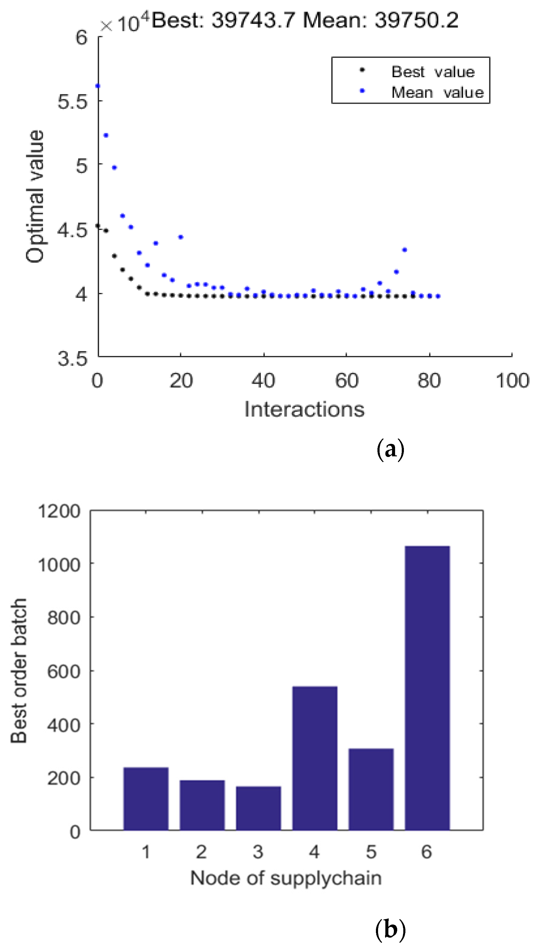
Centralized strategy is the global optimization strategy, which carries out multi-echelon inventory control on the whole fresh product supply chain. This control strategy model is complex. The genetic algorithm is used to optimize the model. In order to obtain the optimal solution, we design the fitness function which conforms to the objective function. The optimal solution is obtained after 83 iterations, as shown in Figure 3 and Table 5.
Figure 3a shows that the minimum inventory cost of the entire supply chain is RMB 39,744 per month. The average inventory cost is RMB 39,750 per month. The centralized strategy is shown in Table 5.

3.4. Results Analysis

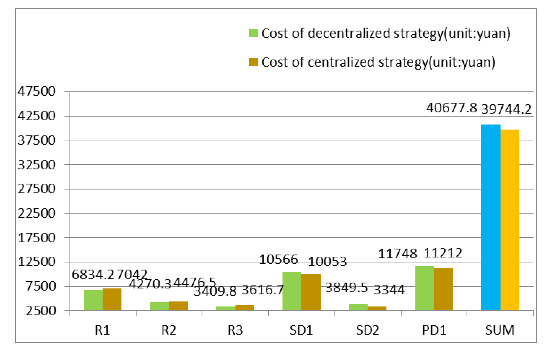
By comparing the two sets of data solved by the decentralized decision model and the centralized decision model, we can see the difference of relevant decision values such as the order quantity, order point, stock cycle, and total cost before and after optimization, as shown in Figure 4 and Figure 5.
The comparison of order batch and cost at each node before and after optimization is shown in Figure 4 and Figure 5.
Some analyses are discussed below:
(1) It can be found that after optimization, the order quantity and stock cycle at all levels are decreased. As shown in Figure 4, Table 4, and Table 5, the order quantity of the retailer and tier 2 distributors obviously decreased, while for the tier 1 distributor it only decreased a little, and remained unchanged for the stock cycle. It can be seen that the full optimization has little impact on node enterprises in the upstream of the supply chain, while there is a more obvious effect on node enterprises in the middle and downstream of the supply chain. Therefore, this optimization model is of more reference significance for retailers and tier 2 distributors to formulate their ordering strategies.
(2) Generally, the stock cycle of fresh products is short. If the goods are stocked for more than three days, they will lose selling value, which results in loss of cost. After optimization, the stock cycle of each node can be lower than 2.5 days, as shown in Table 5. This is in line with the actual storage needs for fresh products.
(3) For the retailers, the cost is increased, as shown in Figure 5, because it is not referred to EOQ. The costs for tier 2 and tier 1 distributors are decreased due to the reduction in ordering quantity, which results in an increased cost for retailers.
(4) It can be found in the given example that after full optimization, the overall inventory costs are reduced from RMB 40,677.8 to RMB 39,744.2. The difference is not that large, because the value of cost coefficients, order quantity, and other data of each enterprise node are small, and the structure of the supply chain system is simple. If this optimization model is applied to a large-scale supply chain, the effect from optimization would be more obvious.
To sum up, the minimization of inventory costs of the entire supply chain cannot be obtained if each enterprise node makes independent decisions. Independent decision-making should be avoided; full optimization should be applied. The centralized strategy model proposed in this paper has practical significance for the optimal inventory management of supply chains.

4. Simulation Model Verification

We obtained an optimal inventory management solution by optimizing the mathematical model. However, we need to verify the effects of the two ordering strategies before and after optimization in practice by simulation. Flexsim is simulation software for discrete event systems. Its functions include the design of a simulation model, the implementation of simulation logic, model validation, and result output and simulation analysis. Many researchers have used Flexsim to solve many practical problems [36,37,38,39,40]. Based on the characteristics of Flexsim, it is very suitable for simulating the logistic process between the warehouse systems at all levels of the supply chain, so we chose Flexsim to simulate the operation effect under both strategies.

4.1. Simulation Model Establish

A simulation model layout for multi-echelon inventory is established, and every 100 units as one day is selected on the simulation time clock. The warm-up period is defined as 700, which equivalent to one week in reality.
In the Flexsim environment, we use the “Queue” as the warehouse of each node in the system to store the “Item” which represents fresh goods.
The “Source” is used to simulate the product supply and the initial inventory of each enterprise node. The customer’s arrival is simulated by the “Source”, while the departure is simulated by the “Sink”. The spoiled product enters the “Sink” directly. "Flexsim Experiment Control" is used to record the inventory amount of each node for 20 simulations. The specific layout is shown in Figure 6.

4.2. Simulation Results Analysis

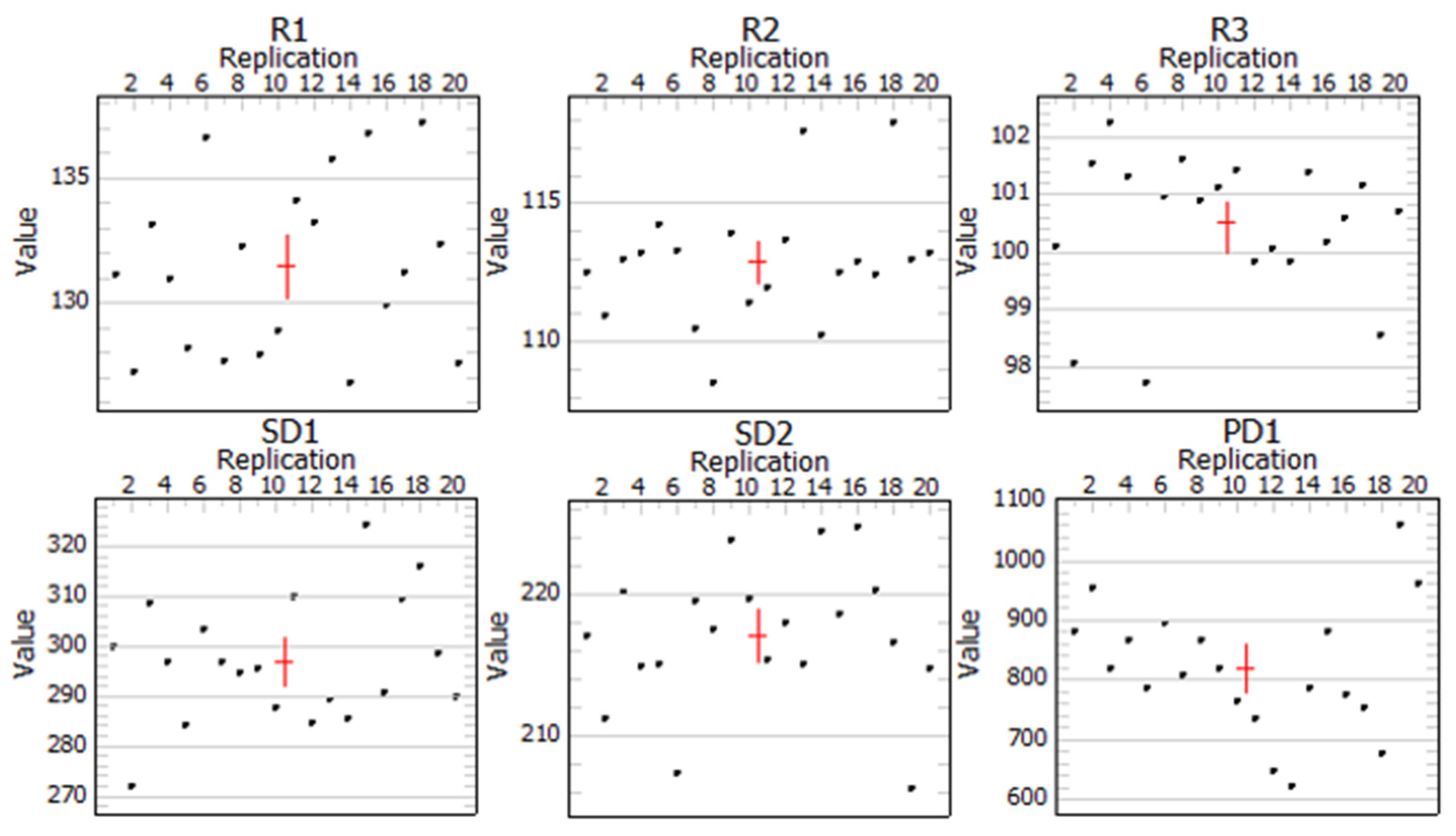
In order to verify the feasibility of strategies using genetic algorithms in the mathematical model, the simulation model was performed 20 times for the two strategies.
The inventory of each enterprise node was selected as the performance index. The average value of inventory at each node of the two strategies by running 20 simulations was recorded with a confidence of 90, as shown in Figure 7 and Figure 8.
The average inventory and the total inventory costs of supply chain were calculated as shown in Table 6.
In the inventory comparison of the simulation results, the centralized strategy optimized by the algorithm performs better than the decentralized strategy of directly solving the lowest inventory cost at all levels, as shown in Table 6:
(1) Due to the reduction in the order quantity, the average inventory of every node at all levels has declined, which not only reduces the inventory holding cost, but also reduces the loss of deterioration of the products;
(2) The ordering costs at retail level slightly increase due to frequent ordering times caused by lower ordering volume. With the gradual increase in demand fluctuations, the reduced inventory maintenance costs for upstream node enterprises are sufficient to compensate for the increased ordering costs of retailers.
(3) The inventory cost (RMB 39,658.5) from the simulation model of the centralized strategy is smaller than that of the decentralized strategy (RMB 39,663.2). It can be seen that the optimized solution from the mathematical model remains better in the simulation model, proving the effectiveness of the multi-echelon inventory model of fresh products established in this paper, and also the effective of the fitness function designed based on the genetic algorithm.
(4) In practice, it is common that the reduction in inventory costs for one node enterprise will lead to an increase in that cost for other node enterprises, but in general, if coordination does not work well, enterprises are not willing to sacrifice their interests for the optimization of the whole supply chain. Therefore, the best strategy is through contracts and other means, by a leading enterprise conducting the overall planning, to avoid each level of independent processing decisions and plans so as to minimize the total inventory cost of the whole supply chain.
In this study, some decision values solved by the mathematical model, such as the order quantity, order point, and demand of each enterprise node, were taken as the input conditions for a simulation. The simulation was carried out according to the supply process in the actual supply chain environment. After 20 simulations, the average inventory volume and inventory costs of each node were obtained. By comparing the simulation output values of the two inventory control strategies, we find that the total cost value of the centralized strategy model is still lower than that of decentralized strategy. It is proved that the optimized inventory control strategy is better for cost-saving in actual operation. An optimized inventory control strategy can provide reference and direction for the practical link of supply chain inventory management, and has practical management significance.

5. Conclusions and Further Research

5.1. Conclusions

In this study, we used the principle of inventory control model, combined with the influence of perishable product deterioration, and established a multi-echelon inventory mathematical model to assist fresh product inventory decisions.
Taking a small supply chain composed of five enterprise nodes as an example, the decentralized strategy is used to exercise independent decisions for each layer through the mathematical model, obtaining the partial optimal strategy. We then designed a fitness function, using Matlab for iteration by genetic algorithm, to find the optimal strategy for the whole system, namely the centralized strategy.
By substituting the strategies before and after optimization into the Flexsim simulation model for verification, it can be found that the optimal solution in the mathematical model still has a good effect in the simulation model. It proves that the multi-echelon fresh product inventory model established in this study is feasible, and the fitness function selected in the genetic algorithm is effective.
The results of this study will assist supply chain managers in the fresh food industry to make decisions to maximize total profits, while also providing the freshest food to customers.

5.2. Limitations and Future Research

(1) Although the problem of deterioration was taken into account in the model establishment in this paper, the model only considered the situation for a constant deterioration rate; other deterioration conditions were not considered.
(2) In this paper, we only considered one kind of product for the multi-echelon inventory optimization of the supply chain. Therefore, future work could consider the interaction of multiple products in inventory optimization.
(3) The case quoted in this paper only considered the model application and simulation of the six node enterprises in a three-level supply chain; the data scale is comparatively small. Future applications for more complex supply chains and more node control problems will be considered.

Author Contributions

Conceptualization, methodology, software, validation, writing—original draft preparation, Y.Z.; formal analysis, investigation, data curation, Y.Z. and L.M.; writing—review and editing, supervision, Y.C. All authors have read and agreed to the published version of the manuscript.

Funding

This research received no external funding.

Data Availability Statement

All data and models generated or used during the study appear in the submitted article.

Conflicts of Interest

The authors declare no conflict of interest.

References

  1. Olsson, F. Modelling two-echelon serial inventory systems with perishable items. IMA J. Manag. Math. 2010, 21, 1–17. [Google Scholar] [CrossRef]
  2. Mo, J.T.; Chen, G.M.; Fan, T.; Mao, H. Optimal ordering policies for perishable multi-item under stock-dependent demand and two-level trade credit. Appl. Math. Model. 2014, 38, 2522–2532. [Google Scholar]
  3. Kaya, O.; Ghahroodi, S.R. Inventory control and pricing for perishable products under age and price dependent stochastic demand. Math. Methods Oper. Res. 2018, 88, 1–35. [Google Scholar] [CrossRef]
  4. Rijpkema, W.A.; Roberto, R.; van der Vorst, J.G.A.J. Effective Sourcing Strategies for Perishable Product Supply Chains. Int. J. Phys. Distrib. Logist. Manag. 2014, 44, 494–510. [Google Scholar] [CrossRef] [Green Version]
  5. Zheng, Q.; Ieromonachou, P.; Fan, T.J.; Zhou, L. Supply chain contracting coordination for fresh products with fresh-keeping effort. Ind. Manag. Data Syst. 2017, 117, 538–559. [Google Scholar] [CrossRef]
  6. Janssen, L.; Diabat, A.; Sauer, J.; Herrmann, F. A stochastic micro-periodic age-based inventory replenishment policy for perishable goods. Transp. Res. Part E Logist. Transp. Rev. 2018, 118, 445–465. [Google Scholar] [CrossRef]
  7. Clark, A.J.; Scarf, H. Optimal polices for multi-echelon inventory problem. Manag. Sci. 1960, 6, 475–490. [Google Scholar] [CrossRef]
  8. Duong, L.N.; Wood, L.C.; Wang, W.Y. Effects of consumer demand, product lifetime, and substitution ratio on perishable inventory management. Sustainability 2018, 10, 1559. [Google Scholar] [CrossRef] [Green Version]
  9. Hill, R.M. The single-vendor single-buyer integrated production inventory model with a generalized policy. Eur. J. Oper. Res. 1997, 97, 493–499. [Google Scholar] [CrossRef]
  10. Weng, Z.K. Modeling quantity discounts under general price-sensitive demand function: Optimal policies and relationships. Eur. J. Oper. Res. 1995, 86, 300–314. [Google Scholar] [CrossRef]
  11. Diks, E.B.; De Kok, A.G. Optimal control of a divergent multi-echelon inventory system. Eur. J. Oper. Res. 1998, 111, 75–97. [Google Scholar] [CrossRef]
  12. Moinzadeh, K. A multi-echelon inventory system with information exchange. Manag. Sci. 2002, 48, 414–426. [Google Scholar] [CrossRef] [Green Version]
  13. Giannoccaro, I.; Pontrandolfo, P.; Scozzi, B. A fuzzy echelon approach for inventory management in Supply chains. Eur. J. Oper. Res. 2003, 149, 185–196. [Google Scholar] [CrossRef]
  14. Chen, J.M.; Chen, T.H. The multi-item replenishment problem in a two-echelon supply chain: The effect of centralization versus decentralization. Comput. Oper. Res. 2005, 32, 3191–3207. [Google Scholar] [CrossRef]
  15. Wang, Y.C.; Geng, X.X.; Zhang, F. An immune genetic algorithm for multi-echelon inventory cost control of IOT based supply chains. IEEE Access 2018, 6, 8547–8555. [Google Scholar] [CrossRef]
  16. Presbitero, A.; Krzhizhanovskaya, V.; Mancini, E.; Brands, R.; Sloot, P. Immune system model calibration by genetic algorithm. Proc. Comput. Sci. 2016, 101, 161–171. [Google Scholar] [CrossRef]
  17. Iida, T. The infinite horizon non-stationary stochastic multi-echelon inventory problem and near-myopic policies. Eur. J. Oper. Res. 2001, 134, 525–539. [Google Scholar] [CrossRef]
  18. Mandel, A.; Vilms, M. Local supply chain control model with unreliable suppliers. IFAC Pap. Online 2016, 49, 437–442. [Google Scholar] [CrossRef]
  19. Wang, L.L.; Zhang, T.; Guo, Y. Under the environment of agile supply chain inventory control research. Adv. Mater. Res. 2014, 945–949, 3179–3182. [Google Scholar] [CrossRef]
  20. Ech-Cheikh, H.; Elhaq, S.L.; Rachid, A.; Douraid, A. Simulating demand uncertainty and inventory control variability of multi-echelon distribution supply chain. Int. J. Appl. Logist. 2014, 5, 12–31. [Google Scholar] [CrossRef]
  21. Goswami, M.; Daultani, Y.; De, A. Decision modeling and analysis in new product development considering supply chain uncertainties: A multi-functional expert based approach. Expert Syst. Appl. 2021, 166, 114016. [Google Scholar] [CrossRef]
  22. De, A.; Mogale, D.; Zhang, M.; Pratap, S.; Kumar, S.K.; Huang, G.Q. Multi-period multi-echelon inventory transportation problem considering stakeholders behavioural tendencies. Int. J. Prod. Econ. 2020, 225, 107566. [Google Scholar] [CrossRef]
  23. Choudhary, A.; De, A.; Ahmed, K.; Shankar, R. An integrated fuzzy intuitionistic sustainability assessment framework for manufacturing supply chain: A study of UK based firms. Ann. Oper. Res. 2021. [Google Scholar] [CrossRef]
  24. Ray, A.; De, A.; Mondal, S.; Wang, J.W. Selection of best buyback strategy for original equipment manufacturer and independent remanufacturer—Game theoretic approach. Int. J. Prod. Res. 2020, 7, 1–30. [Google Scholar] [CrossRef]
  25. Pourhejazy, P.; Kwon, O.K. The new generation of operations research methods in supply chain optimization: A review. Sustainability 2016, 8, 1033. [Google Scholar] [CrossRef] [Green Version]
  26. Schwartz, J.D.; Wang, W.; Rivera, D.E. Simulation-based optimization of process control policies for inventory management in supply chains. Automatica 2006, 42, 1311–1320. [Google Scholar] [CrossRef]
  27. Chu, Y.; You, F.; Wassick, J.M.; Agarwal, A. Simulation-based optimization framework for multi-echelon inventory systems under uncertainty. Comput. Chem. Eng. 2015, 73, 1–16. [Google Scholar] [CrossRef]
  28. Attar, A.; Raissi, S.; Khalili-Damghani, K. Simulation-optimization approach for a continuous-review, base-stock inventory model with general compound demands, random lead times, and lost sales. Simul. Transp. Soc. Model. Simul. Int. 2016, 92, 547–564. [Google Scholar] [CrossRef]
  29. Lee, Y.H.; Kim, S.H.; Moo, C. Production distribution planning in supply chain using a hybrid approach. Prod. Plan. Control 2002, 13, 35–46. [Google Scholar] [CrossRef]
  30. Kochel, P.; Nielander, U. Simulation-based optimization of multi-echelon inventory systems. Int. J. Prod. Econ. 2005, 93–94, 505–513. [Google Scholar] [CrossRef]
  31. Heidary, M.H.; Aghaie, A.; Jalalimanesh, A. A simulation-optimization approach for a multi-period, multi-objective supply chain with demand uncertainty and an option contract. Simul. Transp. Soc. Model. Simul. Int. 2018, 94, 649–662. [Google Scholar] [CrossRef] [Green Version]
  32. Zhao, W.D.; Wang, D.W. Simulation-based optimization on control strategies of three-echelon inventory in hybrid supply chain with order uncertainty. IEEE Access 2018, 6, 54215–54223. [Google Scholar] [CrossRef]
  33. Avci, M.G.; Selim, H. A multi-objective simulation-based optimization approach for inventory replenishment problem with premium freights in convergent supply chains. Omega 2018, 80, 153–165. [Google Scholar] [CrossRef]
  34. Gueller, M.; Uygun, Y.; Noche, B. Simulation-based optimization for a capacitated multi-echelon production-inventory system. J. Simul. 2015, 9, 325–336. [Google Scholar] [CrossRef]
  35. Thammatadatrakul, P.; Chiadamrong, N. Optimal inventory control policy of a hybrid manufacturing-remanufacturing system using a hybrid simulation optimisation algorithm. J. Simul. 2019, 13, 14–27. [Google Scholar] [CrossRef]
  36. Xu, G.Y.; Feng, J.H.; Chen, F.L.; Wang, H.; Wang, Z.F. Simulation-based optimization of control policy on multi-echelon inventory system for fresh agricultural products. Int. J. Agric. Biol. Eng. 2019, 12, 184–194. [Google Scholar] [CrossRef] [Green Version]
  37. Bardzinski, P.J.; Walker, P.; Krol, R. Simulation of random tagged ore fow through the bunker in a belt convering system. Int. J. Simul. Model. 2018, 17, 597–608. [Google Scholar] [CrossRef]
  38. Jiao, Y.L.; Xing, X.C.; Zhang, P. Multi-objective storage location allocation optimization and simulation analysis of automated warehouse based on multi-population genetic algorithm. Concurr. Eng. Res. Appl. 2018, 26, 367–377. [Google Scholar] [CrossRef]
  39. Grzybowska, K.; Kovacs, G. The modelling and design process of coordination mechanisms in the supply chain. J. Appl. Log. 2017, 24, 25–38. [Google Scholar] [CrossRef]
  40. Kierzkowski, A.; Kisiel, T. Simulation model of security control system functioning: A case study of the Wroclaw Airport terminal. J. Air Transp. Manag. 2017, 64, 173–185. [Google Scholar] [CrossRef]
Figure 1. Multi-echelon inventory system of fresh products.
Sustainability 13 06309 g001
Figure 2. Multi-echelon inventory system of a fresh product supply chain.
Sustainability 13 06309 g002
Figure 3. Diagram of supply chain optimization. (a) Optimized curve of total inventory cost. (b) Optimized order batch of each node.
Sustainability 13 06309 g003
Figure 4. Order batch at each node of the supply chain before and after optimization.
Sustainability 13 06309 g004
Figure 5. Cost at each node of the supply chain before and after optimization.
Sustainability 13 06309 g005
Figure 6. Multi-echelon inventory simulation layout of fresh products.
Sustainability 13 06309 g006
Figure 7. The inventory map of each enterprise node before optimization.
Sustainability 13 06309 g007
Figure 8. The inventory map of each enterprise node after optimization.
Sustainability 13 06309 g008
Table 1. Cost used in the model.
SymbolDescription
CSInventory maintaining inventory cost refers to the expenses necessary to maintain inventory, that is, the costs incurred because inventory exists to ensure the continuity of production and supply.
COOrder cost refers to the cost of the purchase order issued by the upstream supplier.
CFTransportation cost refers to the cost of transporting items from the upstream inventory to the downstream inventory, and is proportional to the number of transportation and the single transportation volume. It is mainly determined by the price of a single transportation unit.
CPPurchase cost refers to the cost of purchasing the item itself.
CLShortage cost refers to the loss caused by insufficient inventory. The cost can be ignored if the shortage is not allowed.
Table 2. Notations used in the model.
SymbolDescriptionSymbolDescription
θ i j Deterioration rate of ith level, jth node T i j Stock cycle of ith level, jth node
I ( t ) i j Inventory of ith level, jth node at time t C S i j Storage cost per unit time of ith level, jth node
D i j Demand amount of ith level, jth node C O i j Order cost per unit time of ith level, jth node
Q i j Order quantity of ith level, jth node C F i j Transportation cost per unit time of ith level, jth node
R i j Inventory quantity of ith level, jth node when the order is placed C P i j Purchase cost per unit time of ith level, jth node
s i j Storage cost per unit of product per unit of time of ith level, jth node C Total cost of each node of the supply chain in time T
o i j One-time order cost of ith level, jth node n i j Number of orders in cycle T of ith level, jth node
f i j Transportation cost per unit of product per unit of time of ith level, jth node T Supply chain management cycle
p i j Unit purchasing price of unit product of ith level, jth node τ i j Order lead time of ith level, jth node
Table 3. Relevant parameters of the multi-echelon inventory system.
Node s i j /
yuan · kg 1 · d 1
o i j /
yuan · time 1
f i j /
yuan · kg 1
p i j /
yuan · kg 1
τ i j /
d
D i j /
kg · d 1
θ i j
R1 0.04100.1112000.1
R20.04100.1111250.1
R30.04100.1111000.1
SD10.03200.090.81.50.1
SD20.03200.090.81.50.1
PD10.02300.080.61.80.1
Table 4. Decentralized strategy at all levels of the supply chain.
Node Q i j / kg R i j / kg T i j / d C i j / yuan
R1 2892091.356834.2
R22301311.684270.3
R32061051.873409.8
SD16165661.6210,566
SD23521782.783849.5
PD1107710001.9311,748
Table 5. Centralized strategy at all levels of the supply chain.
Node Q i j / kg R i j / kg T i j / d C i j / yuan
R1 2382101.127042.0
R21891311.404476.5
R31661051.533616.7
SD15615591.5010,053.0
SD23071752.503344.0
PD110669781.9411,212.0
Table 6. The average inventory and cost of each enterprise node before and after optimization.
NodeInventory (unit: kg)Cost (unit: yuan)
Before OptimizationAfter OptimizationBefore OptimizationAfter Optimization
R1131.5109.56974.77010.2
R2112.992.34446.54438.8
R3100.580.83579.63602.4
SD1297.0280.09949.89991.3
SD2217.1197.73352.23341.9
PD1820.069811,360.411,274.0
Total cost 39,663.239,658.5
Publisher’s Note: MDPI stays neutral with regard to jurisdictional claims in published maps and institutional affiliations.