Minimum Wage and Household Consumption in Canada: Evidence from High and Low Wage Provinces

Abstract

The minimum wage is a major factor for the successful implementation of much of the sustainable development goals (SDGs). The present research will investigate whether minimum wage (MW) as a sustainable wage policy improves household consumption. Thus, a panel-based analysis comparing high wage (Alberta, British Columbia, Ontario, and Saskatchewan) and low wage provinces (Manitoba, New Brunswick, Newfound land/Lab, Nova Scotia, Prince Edward Island, and Quebec) is employed for the Canadian case within the study period from 1981 to 2019. We analyze the long-term and short-term effects of MW on household consumption using the Dynamic Autoregressive Distributed Lag techniques of the Pooled Mean Group, Dynamic Fixed Effects, and Mean Group estimators. Results show that the long-term impact of MW on household consumption is positive in both the low- and high-wage provinces. The short-term effect is negative in both wage groups, but not significant for the low-wage group. This offers significant debate on the relevance of the MW towards economic stabilization and consumption-led growth.

1. Introduction

The debate on whether the implementation of national minimum wage (MW) laws can lead to improved welfare and, subsequently, the stimulation of economic activities has been controversial. These controversies are associated with the growing discussions on whether the MW could stimulate aggregate demand or lead to inflationary effects—especially during economic recessions such as the recent one induced by the global pandemic of COVID-19. The MW can be perceived as the core foundation on which most of the sustainable development goals (SDGs) are anchored. This is because poverty reduction (goal one), zero hunger (goal two), quality health and well-being (goal three), quality education (goal four), gender equality (goal five), clean water and sanitation (goal six), affordable and clean energy (goal seven), decent work and economic growth (goal eight and nine), reduced inequality (goal ten), as well as responsible production and consumption are all core tenets of sustainable development, which require sustainable wage levels in varying degrees.

The proponents of MW argue that the MW raises the prosperity of all workers, lowers income inequality, and improves the overall performance of the economy [1,2]. Ref. [1] explores the influence of the MW and explains how it influences the distribution of wages. He found that part of this increase is due to reductions in the real MW at the lower part of the distribution. Ref. [2] demonstrate that the federal MW hinders growth and temporarily eliminates rises in wage inequality in the United States. Additionally, heterodox economists argue that an increase in MW would help to raise workers’ incomes and thus boost aggregate demand in the economy [3].

In Canada, most of the studies on the impact of the MW on economic variables demonstrate a negative employment effect of the MW [4,5]. While the relationship between the MW and employment has been explored in the previous studies, little is known about the linkage between the MW and household consumption in Canada. To our understanding, [6] work is the only study on the MW and consumption relationship in Canada. The consumption variable, as used in [6], is proxied as real retail trade sales normalized to the adult population and results indicate a positive long-term relationship between the MW and the real values of retail sales trade.

This research extends the literature by investigating the relationship between the MW and household consumption in Canada. Canada presents an interesting case as it is one of the few North American countries that has adopted a robust provincial minimum wage legislation. This allows provinces the complete jurisdiction over minimum wage payments. According to [7], there is disemployment heterogeneity between high- and low-wage households, which is translated across the provinces. Such income differences across provinces may also imply differences in consumption patterns and sustained quality of life. Therefore, a more concise perspective of the effect of the minimum wage across households with heterogeneous income levels is paramount towards contributing to SDGs 8 and 10 on inequality reduction within and between countries and drive economic growth through wage-led fiscal policies.

This paper is, to our comprehension, the first analysis that takes into account the heterogeneity within Canada’s MW framework. It considers provincial heterogeneity in MW policies in the analysis of the relationship between the MW and consumption at the household level in Canada. Additionally, it employs a more robust empirical methodology than the previous analysis by [6], since it employs panel data rather than a pure time-series, which assumes provincial homogeneity. It examines the effect not only over the long-term but also over the short-term, taking into account different wages groups.

Therefore, the present study empirically addresses the following research questions:

• How do changes in the provincial MW relate to consumption at the household level and does this relationship differ across high- and low-wage provinces?
• Are there any differences in the Canadian MW’s short-term and long-term effect on consumption?
• In Canada, is the MW an effective fiscal policy tool for aggregate demand and economic growth?

We use panel model estimation techniques of the Pooled Mean Group, the Mean Group, and the Dynamics Fixed Effects estimators to achieve our investigative goal of comparing high-wage provinces in (Alberta, British Columbia, Ontario, and Saskatchewan) and low-wage provinces (Manitoba, New Brunswick, Newfoundland/Lab, Nova Scotia, Prince Edward Island, and Quebec) for the period between 1981 and 2019.

The results indicate that the MW has a negative impact on household consumption in the short-term for both wage groups but is not significant for the low-wage group. However, in the long-term, the MW has a positive and significant effect on household consumption in both low- and high-wage groups.

The research continues in the following sections: In Section 2, we discuss the theoretical framework. The literature review is mentioned in Section 3. Section 4 outlines the data and econometric model. The results and discussions are in Section 5 while the last section concludes the study.

2. Theoretical Framework

Refs. [8,9,10,11] were all inspired by the determinants of consumption expenditure. These factors include income, wealth, interest rates, capital gains, and liquid assets. The link between income and consumer expenditure was hypothesized in a conceptual innovation by [8]. Keynes’ proposition contained three relevant points. First, consumption expenditure is principally dependent on absolute income. Second, consumption is positively related to the absolute level of current income, and third, a higher income obtained in a particular period will induce more consumption for that particular [12].

Duesenberry, however, recommended another theory in 1949. Ref. [9] theorized that the present level of consumption is not just induced by the present level of absolute and relative income. It is also induced by past levels of consumption.

In 1957, a hypothesis regarding consumption behavior, which was termed the permanent income hypotheses, was postulated by Friedman. According to Friedman’s hypothesis, as the wage increases, consumers will not raise their consumption.

Another theory was put forward by [11] in the early 1950s, which was termed the life-cycle hypothesis. It stipulated that future income expectations over the whole life cycle is determined mostly through current income. Modigliani’s life-cycle model assumes that individuals plan their consumption and savings to optimize overall utility over the lifetime of a person and they smooth their consumption in a lifetime [13] Thus, with an emphasis on the different relationships between the MW and household consumption across high and low wage groups in the long- and short-term, Modigliani’s life-cycle theory explains more relevantly the short-term negative impact of the MW on household consumption and the long-term positive effect.

3. Literature Review

The empirical research on the relationship between consumption and MWs is lacking and few studies are addressing the impact of MWs on consumption. For MW-based U.S. households, [14] found a positive spending effect and concluded that much of the consumption is driven by the purchases of vehicles. This trend is seen among low-income households which confirm some constraints due to borrowing and coping costs. Likewise, [15] uses sales data of the United States to assess the impact of the MW on consumption and he found that a 10 percent rise in MWs raises non-durable consumption by 1 percent at the county level and demonstrates that the rise in poorer counties is larger. Ref. [16] found that MW rises are positively associated with consumption among low-income households in China. This positive effect was driven by major expenditure on health care and the education of household members.

For Canadian studies, [17] structural general equilibrium simulation suggests higher inflation induced by higher price levels. Such inflation rates are due the MW increase over the years (2018 and 2019). An increase in inflation will trigger an increase in interest rates. Their findings suggest a slight decrease in consumption. However, the findings of Jung et al.’s paper investigates the relationship between the MW and consumption, which is proxied by real retail trade normalized to the adult population and shows that a one percentage point rise in the actual MW is correlated with a 0.5 percentage point increase in the real retail trade. Jung et al.’s investigations confirm that the MW boosts consumption and hence economic growth. Thus, the present study is in line with Jung et al.’s research and it examines the relationship between MW and consumption on the household level to gain a deeper overview of the MW’s impact and related policy implications. A different methodology and wage category was used to determine the effects of MW increases on consumption at the household level.

4. Data and Methodology

The study included a panel of six low-wage provinces (New Brunswick, Newfoundland/Lab, Manitoba, Nova Scotia, Quebec, and Prince Edward Island) and four high-wage provinces (Alberta, British Columbia, Saskatchewan, and Ontario) of Canada from 1981 to 2019 and the data was obtained from the database of Statistics Canada. The variable definition overview is outlined in

Table 1. Variables.

Indicator	Symbol	Source
Household final consumption expenditure (in 2012 millions of CAD)	HCON	Statcan
Real MW (measured in 2012 CAD)	MW	Statcan
Gross domestic product per capita, income-based (measured in 2012 thousands of CAD)	GDPC	Statcan
Interest received on consumer credit	RINT	Statcan
Final domestic demand (in 2012 millions of CAD)	DEMND	Statcan
Percentage of individuals in low income	LOW_INCME	Statcan

Note: CAD denotes Canadian Dollars. Source: Statistics Canada 2019.

.

In this study Household, final consumption expenditure is the dependent variable. The empirical models often involve several control variables. The five major determinants of consumer expenditure are current disposable income, household equity, projected future income, price level, and interest rates. While choosing control variables, two main factors are taken into account. First, control variables that influence consumption demand are chosen. Second, control variables that are commonly known as determinants of both low wage and high wage are selected in order to compare the effects of economic policy on household consumption separately. The variables that were used for control purposes are as follows: the real minimum wage, GDP per capita, interest–consumer credit, domestic demand, and percentage of individuals in low income are independent variables. The term “real household final consumption expenditure” refers to all purchases made by resident households to fulfill their daily needs. The minimum wage in real terms is reported in 2012 CAD. The Gross Domestic Product (GDP) per capita in real terms is measured in 2012 thousands of CAD. The interest received on consumer credit is the amount of expenses on consumer credit accounts such as private student loans, vehicle loans, and consumer debt. The real domestic demand is the overall amount spent by individuals, businesses, and the government on goods and services. People with lower incomes are defined by the percentages of individuals in low income who earn less than half of the adjusted median household income.

4.1. Differences between High- and Low-Wage Provinces in Canada

Canada is divided into three regions: Atlantic (Newfoundland, Prince Edward Island, Nova Scotia, and New Brunswick), Central (Ontario and Quebec), and Western (Manitoba, Saskatchewan, Alberta, and British Columbia). As [18] states, Canadian data are well-suited for analyzing minimum wage effects because they cover a long period and contain both time-series and cross-sectional variance in minimum wage changes.

According to the 2015 Federal Jurisdiction Workplace Survey (FJWS) and the Labour Force Survey (LFS), three of the four provinces with the largest concentration of federal institutions have a minimum wage of about $15 per hour (Alberta, British Columbia, and Ontario). Three of Canada’s four most populated provinces lack a program of temporal variation (namely, British Columbia, Quebec, and Alberta). The minimum wage in British Colombia was increased by 28 percent through one year in May 2011 [19]. Recently, Ontario has increased the minimum wage by 21%. In 2018, there are significant differences in the average and median incomes across provinces [19].

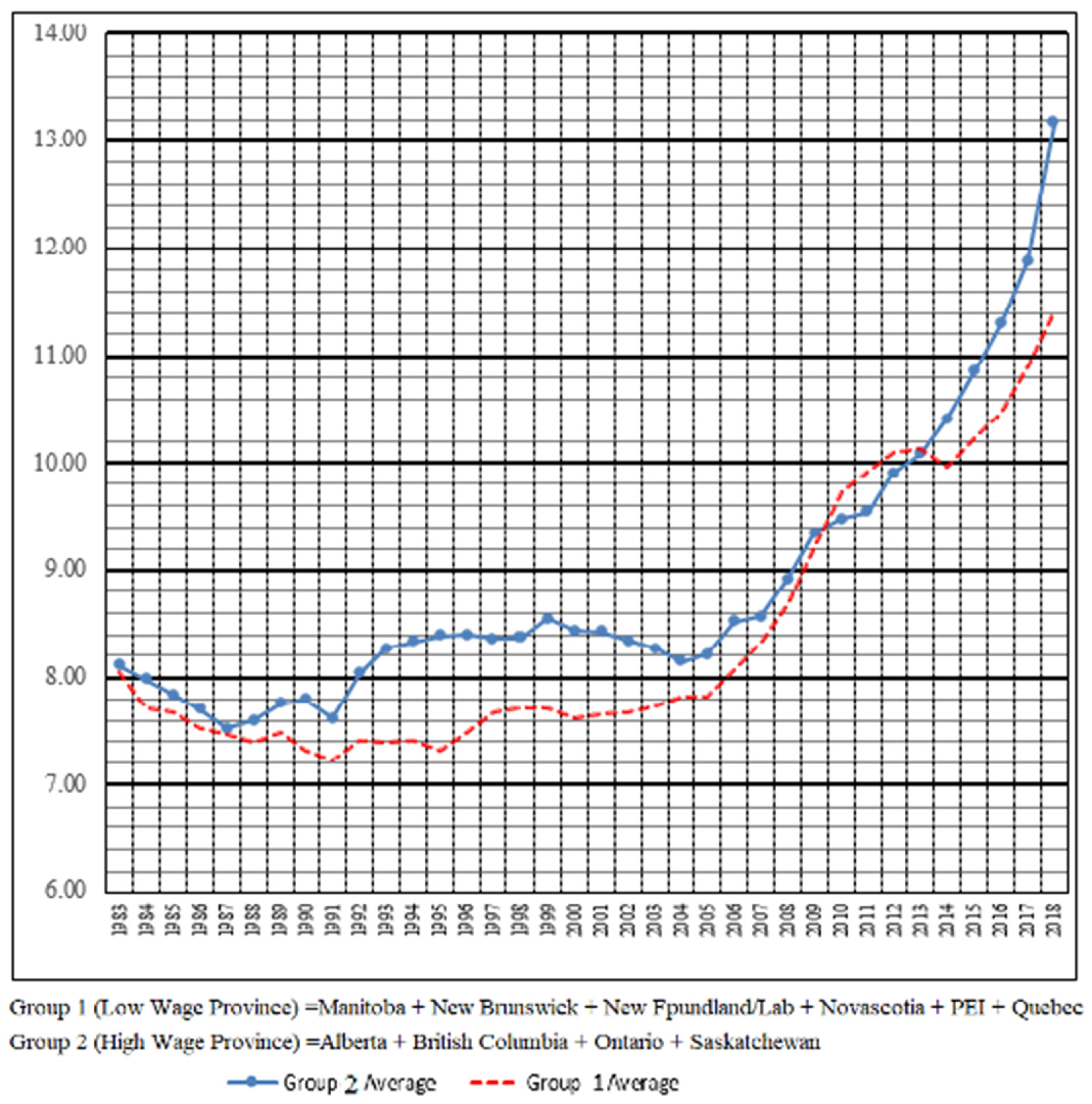
A similar image appears in the comparison of the low-wage provinces (Manitoba, New Brunswick, Newfoundland/Lab, Nova Scotia, Quebec, and Prince Edwards Island) and the high-wage provinces as a group (Alberta, Saskatchewan, Ontario, and British Colombia). Differences in the MW across provinces could also result in varying trends of household consumption, GDP per capita, and interest rates. We explore these potential differences by demarcating provinces as low-wage provinces (Group 1) and high-wage provinces (Group 2) while evaluating the effect of the MW on Canadian household consumption.

Figure 1 shows that both the high- and low-wage provinces had a CAD 8.00 MW in 1983. They have slightly decreased and increased until 2004, but since then, they have shown a sharp upward slope. Of course, the increased slope of Group 2 has been higher, so that in 2018, Group 2 is about 1.6 points higher than Group 1.

In Figure 2, we see that there is a big difference in household consumption between the two groups. Group 1 has increased by only 10% in these 35 years while Group 2 rises about three times more in this period.

In Figure 3, a sharp fluctuation is seen for the interest rates in Group 2, but Group 1 has less fluctuation. Throughout the study period, Group 2 is significantly higher than Group 1. The interesting thing about this chart is that both groups have increased and decreased in the same years, and at the same time, and have a similar pattern in this regard. Both groups had a large increase in GDP.

In Figure 4 until 2014 when they decreased. Of course, until 2014, both groups had ups and downs that had a similar pattern. However, after 2014, the rate of decrease in Group 1 is much higher than in Group 2.

Since these two groups also vary in terms of GDP per capita, household consumption, and interest rates, as shown in the figures, further research is required to determine the interaction between ther MW and household consumption and to decide if a low MW is linked to high household consumption. We would like to unravel the MW–household dynamics because, according to the theory, different results are predicted in two different groups of high- and low-income groups, and therefore it is preferable if they are studied differently to uncover the potential differences, not only in their income level, but also in their consumption and GDP per capita level. Thus, investigating them differently can uncover novel results.

4.2. Methodology

4.2.1. Model

This research aims to use a multivariate panel-based model to investigate the long-term association between household consumption and the minimum wage while controlling for domestic demand, interest–consumer credit, the percentage of individuals in low-income groups, and GDP per capita. The empirical model is defined as below for our analysis:

LHCON_i,t = f(LMW_it, LDEMND_it, LRINT_it, Low_INCME_it, LGDPC_it)

(1)

The above equation has a linear relationship and can be used to model consumption (total provinces, low-wage provinces, and high-wage provinces) in relation to the effect of minimum wage when controlling for other explanatory variables.

Model 1:

$${\mathrm{TLHCON}}_{\mathrm{i},\mathrm{t}}={\beta }_0+ {\beta }_1\mathrm{L}{\mathrm{MW}}_{\mathrm{i},\mathrm{t}},+ {\beta }_2{\mathrm{LDEMND}}_{\mathrm{it}}+ {\beta }_3{\mathrm{LRINT}}_{\mathrm{i},\mathrm{t}}+ {\beta }_4\mathrm{Low}\_{\mathrm{INCME}}_{\mathrm{it}}+ {\beta }_5{\mathrm{LGDPC}}_{\mathrm{i},\mathrm{t}}{}_{+}{\epsilon }_{i,t}$$

(2)

Model 2:

$${\mathrm{LLHCON}}_{\mathrm{i},\mathrm{t}}={\beta }_0 + {\beta }_1\mathrm{L}{\mathrm{MW}}_{\mathrm{i},\mathrm{t}}, + {\beta }_2{\mathrm{LDEMND}}_{\mathrm{it}} + {\beta }_3{\mathrm{LRINT}}_{\mathrm{i},\mathrm{t}} + {\beta }_4\mathrm{Low}\_{\mathrm{INCME}}_{\mathrm{it}} + {\beta }_5{\mathrm{LGDPC}}_{\mathrm{i},\mathrm{t}}{}_{+}{\epsilon }_{i,t}$$

(3)

Model 3:

$${\mathrm{HLHCON}}_{\mathrm{i},\mathrm{t}}={\beta }_0 + {\beta }_1\mathrm{L}{\mathrm{MW}}_{\mathrm{i},\mathrm{t}}, + {\beta }_2{\mathrm{LDEMND}}_{\mathrm{it}} + {\beta }_3{\mathrm{LRINT}}_{\mathrm{i},\mathrm{t}} + {\beta }_4\mathrm{Low}\_{\mathrm{INCME}}_{\mathrm{it}} + {\beta }_5{\mathrm{LGDPC}}_{\mathrm{i},\mathrm{t}}{}_{+}{\epsilon }_{i,t}$$

(4)

The estimations are based on the logarithmic forms of the variables; Models 1, 2, and 3 reflect total, low-wage, and high-wage provinces in Canada, respectively. The estimated regressor coefficients are given by ${\beta }_k$(k = 0, 1, ≠, 5), and the error term is given by ${\epsilon }_{i,t}$.

4.2.2. Cross-Sectional Dependence (CD) Test

When doing a panel data study, one of the most relevant diagnostic tests that researchers can employ is the cross-sectional dependence test that tests for the use of first-generation estimations over the second-generation estimations [20,21]. The CD tests used in this analysis had the following general equations, and the results are shown in

Table 2. Cross-section dependence test.

Test	Constant		Trend
	Statistic	p-Value	Statistic	p-Value
LM	150.1	0.0000	188.9	0.0000
LMadj *	32.08	0.0000	42.44	0.0000
LMCD *	6.825	0.0000	10.59	0.0000

* Two-sided test.

.

$$C{D}_{LM}=T{{\displaystyle \sum }}_{i=1}^{N-1}{{\displaystyle \sum }}_{j=i+1}^N{\widehat{p}}_{ij}^2$$

(5)

$$C{D}_P=\sqrt{\frac{2T}{N\left(N-1\right)}} \left({{\displaystyle \sum }}_{i=1}^{N-1}{{\displaystyle \sum }}_{j=i+1}^N{\widehat{p}}_{ij}\right)$$

(6)

$$C{D}_{LMad}=\sqrt{\frac{2}{N\left(N-1\right)}}{{\displaystyle \sum }}_{i=1}^{N-1}{{\displaystyle \sum }}_{j=i+1}^N\frac{{\widehat{p}}_{ij}^2-{\mu }_{Tij}}{v_{tij}}$$

(7)

4.2.3. Panel Unit Root Tests

We use [22] second-generation panel unit root tests to check if the variables are sensitive to cross-sectional dependence (i.e., Cross-sectional Augmented test, [23] test (CIPS), and cross-sectional augmented Dickey–Fuller (CADF) [22]. The presence of the cross-sectional dependency and/or slope heterogeneity could bias the results. The CADF and CIPS tests have the following general equation forms. The results are shown in

Table 3. Results of the CADF and CIPS unit root tests.

Variables	CIPS	CADF
Levels
HCON	−1.128	−1.9893
MWAGE	−1.745	1.1071
RGDPC	−1.919	−1.8023
DEMND	−1.671	−2.3707 ***
LOW-INCME	−2.901 ***	−2.7973 ***
RINT	−2.360 **	−1.9804 **
First difference
HCON	−4.702 ***	−6.6344 ***
MWAGE	−5.307 ***	−5.5049 ***
RGDPC	−5.737 ***	−5.8451 ***
DEMND	−4.438 ***	−6.1834 ***
LOW-INCME	−6.159 ***	−8.2233 ***
RINT	−4.984 ***	−4.3959 ***

Notes: stationary *** at the 1% level; ** at the 5% level.

.

$$\mathrm{CADF}={\mathrm{t}}_{\mathrm{i}}(\mathrm{N},\mathrm{T})= \frac{∆y_i^t{\overline{M}}_{\omega }{y}_{i,-1}}{{\widehat{\sigma }}_i{(y_{i,-1}^t{\overline{M}}_{\omega }{y}_{i,-1})}^{1/2}}$$

(8)

$$\mathrm{CIPS}=\mathrm{t}\text{-}\mathrm{bar}= \frac{1}{N}{{\displaystyle \sum }}_{i=1}^N t_i \left(N,T\right)$$

(9)

4.2.4. Homogeneity

Given that the provinces in Canada apply different minimum wage regimes and different consumption patterns, as found under Figure 1, the need to apply a model that captures these heterogeneous characteristics is warranted. This study also uses [24] test to check whether the slope is homogeneous. The Mean Group Method (MG) estimators are consistent when the slops are heterogeneous. The MG method controls for both short-term and long-term heterogeneity; the Dynamic Fixed-Effect (DFE) method restricts homogeneity in both the short- and long-terms; and the Pooled Mean Group (PMG) method controls for short-term heterogeneity whereas assuming homogeneity in the long-term [25,26]. Data analyzed in

Table 4. Results of homogeneity, heteroskedasticity and autocorrelation Tests.

	Test	Statistics	Probability
Homogeneity	Swamy (1970)	chi2 (5) = 590.41	Prob > chi2 = 0.0000
Heteroskedasticity	Breusch–Pagan/Cook–Weisberg	chi2 (20) = 199.607	Prob > chi2 = 0.0000
Autocorrelation	Wooldridge	F (5385) = 31,623.47	Prob > F = 0.0000

shows that the slope parameters are heterogeneous. As a consequence, it is preferable to use the second generation panel approach, and the results of the Hausman tests indicate that the PMG and MG estimators are more efficient than DFE.

4.2.5. Panel Cointegration Test

This research utilized the [27] cointegration test. The [27] test has an advantage over other cointegration tests because it is based on structural dynamics rather than residuals. The error correction model is used to test the null hypothesis of no cointegration, which is based on the principle that the error correction term is equal to zero in a conditional panel framework. In the model, four different hypotheses are evaluated. The first two statistics, the panel statistics ($P_{\tau }$, $P_{\alpha }$), check that the main interpretation panel as a whole has been cointegrated, while the group means statistics $(G_{\tau }$, $G_{\alpha }$) evaluate the alternate explanation that at least one individual is cointegrated. The panel error correction model for the test is specified as follows:

$$∆{\mathit{y}}_{\mathit{i}\mathit{t}}={\widehat{\mathit{\delta }}}_{\mathit{i}}^{\prime }{\mathit{d}}_{\mathit{t}}+{\widehat{\mathit{\alpha }}}_{\mathit{i}}{\mathit{y}}_{\mathit{i}\mathit{t}-1}+{\widehat{\mathit{\lambda }}}_{\mathit{i}}^{\prime }{\mathit{x}}_{\mathit{i}\mathit{t}}+{\displaystyle \sum }_{\mathit{j}=1}^{{\mathit{p}}_{\mathit{i}}}{\widehat{\mathit{\alpha }}}_{\mathit{i}\mathit{j}}∆{\mathit{y}}_{\mathit{i}\mathit{t}-\mathit{j}}+{\displaystyle \sum }_{\mathit{j}=0}^{{\mathit{p}}_{\mathit{i}}}{\widehat{\mathit{\gamma }}}_{\mathit{i}\mathit{j}}∆{\mathit{x}}_{\mathit{i}\mathit{t}-\mathit{j}}+{\mathit{\epsilon }}_{\mathit{i}\mathit{t}}$$

(10)

The panel statistics ($P_{\tau }$, $P_{\alpha }$) and the group mean statistics ($G_{\tau }$, $G_{\alpha }$) are calculated as follows:

$$P_{\tau }=\frac{\widehat{\alpha }}{SE\left(\widehat{\alpha }\right)},P_{\alpha }=T\widehat{\alpha },$$

(11)

$$G_{\tau }=\frac{1}{N}{\displaystyle \sum }_{i=1}^N\frac{{\widehat{\alpha }}_i}{SE\left({\widehat{\alpha }}_i\right)}$$

(12)

$$G_a=\frac{1}{N}{\displaystyle \sum }_{i=1}^N\frac{T{\widehat{\alpha }}_i}{{\widehat{\alpha }}_i}$$

(13)

The results of the tests are presented in

Table 5. The results of cointegration test.

	Statistic	p-Value
Gt	−2.982	0.006
Ga	−3.71	0.999
Pt	−2.417	0.095
Pa	8.761	0.265

.

4.2.6. Error Correction-Based Panel Estimations

We were able to estimate the long-term parameters of the panel ARDL method developed by [26]. The ARDL model has been defined with an Error Correction Model (ECM) for the specified prediction, and the equation for the model is presented as below:

$$∆LHCO{N}_{i,t}={\delta }_i(LHCO{N}_{i,t-1} -{\theta }_i{T}_{i,t})+{{\displaystyle \sum }}_{j=1}^{ p-1} {\gamma }_{iJ}∆LHCO{N}_{i,t-j} + {{\displaystyle \sum }}_{j=0}^{q-1} {\theta }_{iJ}∆T_{i,t-j}+{\epsilon }_{i,t}$$

(14)

where:

$${\delta }_i=-(1-{{\displaystyle \sum }}_{j=1}^p {\gamma }_{iJ})=\mathrm{speed}\mathrm{of}\mathrm{adjustment}$$

(15)

$${\theta }_i=-\frac{{{\displaystyle \sum }}_{j=0}^p {\theta }_{iJ}}{(1-{{\displaystyle \sum }}_{j=1}^p {\gamma }_{iJ})}=-\frac{{{\displaystyle \sum }}_j^q {\theta }_{iJ}}{{\delta }_i}$$

(16)

$${\gamma }_{iJ}=-{{\displaystyle \sum }}_{d=j+1}^{ p} {\gamma }_{i,d}$$

(17)

$${\theta }_{iJ}=-{{\displaystyle \sum }}_{d=j+1}^q{\theta }_{id}$$

(18)

The coefficient of adjustment of consumption against deviation from the equilibrium path is given by the first section of Equation (14) = ${\delta }_{i}LHCO{N}_{i,t-1}$ − ${\theta }_i{T}_{i,t}$, which describes the long-term dynamic relationship between household consumption with the independent variables. The vector ${\theta }_i$ is the parameter used to denote the long-term coefficient while ${\mathit{\delta }}_{\mathit{i}}$ is the adjustment speed for the error correction expression. If ${\delta }_i$ < 0, then a long-term causality exists between LHCON_it and the regressors employed in the model. ${{\displaystyle \sum }}_{j=1}^{ p-1} {\gamma }_{iJ}∆LHCO{N}_{i,t-j}$ and ${{\displaystyle \sum }}_{j=0}^{q-1} {\theta }_{iJ}∆T_{i,t-j}$ are the short-term parameters in the model in Equation (14).

This model based on Equation (14) should therefore be defined for the three panels:

$$\begin{gathered} LHCO{N}_{i,t}={{\displaystyle \sum }}_{j=1}^{ p} {\gamma }_{iJ}LHCO{N}_{i,t-j}+{{\displaystyle \sum }}_{j=0}^q {\theta }_{iJ}LM{W}_{i,t-j}+{{\displaystyle \sum }}_{j=0}^q {\theta }_{iJ}{\mathrm{LDEMND}}_{i,t-j}+{{\displaystyle \sum }}_{j=0}^q {\theta }_{iJ}{\mathrm{LRINT}}_{i,t-j}+ \\ {{\displaystyle \sum }}_{j=0}^q {\theta }_{iJ}\mathrm{Low}\_{\mathrm{INCME}}_{i,t-j}+{{\displaystyle \sum }}_{j=0}^q {\theta }_{iJ}{\mathrm{LGDPC}}_{i,t-j}+{\mu }_i+{\epsilon }_{i,t} \end{gathered}$$

(19)

Equation (19), which follows the framework of non-stationary heterogeneous panel data models, employs the following methods: the Dynamic Fixed Effect (DFE), the Mean Group Method (MG), and the Pooled Mean Group (PMG) PMG Method. Except for the intercept term, the DFE estimator assumes homogeneity in the short-term and long-term coefficients across the cross-sections, while the MG estimator simulates the assumption of heterogeneity as proposed by [28]. The PMG estimator allows for short-term heterogeneity by allowing the slope coefficients to differ cross-sectionally, however, the long-term coefficients are constrained to be homogenous [26].

If the slope heterogeneity assumption holds, the PMG estimator becomes inconsistent. Moreover, according to [29], the PMG estimator becomes more efficient relative to the MG estimator once the homogeneity assumption is validated [30].

Therefore, as indicated in

Table 6. Long-term and short-term MG, PMG, and DFE ARDL (1,0,1,0,0,1) results for total Canadian provinces.

	(1)	(2)	(3)
Variables	MG All Provinces	PMG All Provinces	DFE All Provinces
ECT	−0.439 ***	−0.226 ***	−0.164 ***
	(0.059)	(0.059)	(0.029)
Short-term
D.lmwage	−0.016 **	−0.009	0.020 *
	(0.008)	(0.008)	(0.011)
D.ldemnd	0.664 ***	0.686 ***	0.579 ***
	(0.051)	(0.058)	(0.025)
D.lrint	0.015 ***	0.011 **	0.015 ***
	(0.004)	(0.005)	(0.005)
D.Low_INCME	−0.000	0.000	−0.000
	(0.000)	(0.000)	(0.000)
D.lrgdpc	−0.001 ***	−0.001 ***	−0.001 ***
	(0.000)	(0.000)	(0.000)
Long-term
lmwage	0.152 ***	0.233 ***	0.307 ***
	(0.025)	(0.019)	(0.051)
L.ldemnd	0.898 ***	0.724 ***	0.699 ***
	(0.168)	(0.030)	(0.060)
lrint	−0.062	−0.030 **	−0.023
	(0.041)	(0.013)	(0.024)
Low_INCME	0.002 **	−0.000	0.002 *
	(0.001)	(0.001)	(0.001)
L.lrgdpc	0.003	0.002 **	0.006 **
	(0.003)	(0.001)	(0.002)
Constant	0.347 **	0.190 ***	0.149 ***
	(0.147)	(0.047)	(0.043)
Observations	380	380	338
Hausman test	MG vs. PMG
Chi2   17.06   Prob > chi2   0.0044

Standard errors in parentheses *** p < 0.01, ** p < 0.05, * p < 0.1.

and

Table 7. Long-term and short-term MG, PMG ARDL (1,0,1,0,0,1) results for the low-wage and high-wage panel of Canadian provinces.

Variables	Low-Wage Provinces		High-Wage Provinces
	MG	PMG	MG	PMG
ECT	−0.512 ***	−0.309 ***	−0.328 ***	−0.155 ***
	(0.067)	(0.079)	(0.090)	(0.041)
		Short-term estimates
D.lmwage	−0.022 *	−0.001	−0.008 ***	−0.011 ***
	(0.012)	(0.009)	(0.002)	(0.004)
D.ldemnd	0.695 ***	0.650 ***	0.618 ***	0.635 ***
	(0.053)	(0.073)	(0.106)	(0.088)
D.lrint	0.013 ***	0.015 *	0.019 ***	0.009 **
	(0.005)	(0.008)	(0.006)	(0.004)
D.Low_INCME	−0.001 ***	−0.000	0.000	0.000
	(0.000)	(0.000)	(0.001)	(0.000)
D.lrgdpc	−0.000	0.000	−0.001	−0.000 *
	(0.001)	(0.001)	(0.000)	(0.000)
		Long-term estimates
lmwage	0.169 ***	0.244 ***	0.127 ***	0.272 ***
	(0.033)	(0.022)	(0.041)	(0.046)
L.ldemnd	0.706 ***	0.482 ***	1.186 ***	0.940 ***
	(0.087)	(0.046)	(0.383)	(0.080)
lrint	−0.010	−0.020	−0.140	−0.055
	(0.023)	(0.014)	(0.087)	(0.035)
Low_INCME	0.003 ***	0.001 **	0.001	0.004 ***
	(0.001)	(0.001)	(0.002)	(0.001)
L.lrgdpc	0.001	0.003 ***	0.007	0.004
	(0.001)	(0.001)	(0.008)	(0.003)
Constant	0.507 ***	0.547 ***	0.106	−0.018 **
	(0.187)	(0.135)	(0.208)	(0.008)
Observations	228	228	152	152
Hausman test		MG vs. PMG (Low wage)	MG vs. PMG (high wage)
Chi2		0.58	0.21
Prob > chi2		0.9888	0.9990

Standard errors in parentheses *** p < 0.01, ** p < 0.05, * p < 0.1.

, the Hausman specification test is the acceptable and appropriate method to use when deciding between the PMG and MG estimators for the total, high-wage, and low-wage provincial groups.

Table 8. Summary of the long-term and short-term PMG ARDL (1,0,1,0,0,1) results for the low-wage and high-wage panel of Canadian provinces.

Variables	Low-Wage Provinces	High-Wage Provinces
	PMG	PMG
ECT	−0.309 ***	−0.155 ***
	(0.079)	(0.041)
	Short-term estimates
D.lmwage	−0.001	−0.011 ***
	(0.009)	(0.004)
D.ldemnd	0.650 ***	0.635 ***
	(0.073)	(0.088)
D.lrint	0.015 *	0.009 **
	(0.008)	(0.004)
D.Low_INCME	−0.000	0.000
	(0.000)	(0.000)
D.lrgdpc	0.000	−0.000 *
	(0.001)	(0.000)
	Long-term estimates
lmwage	0.244 ***	0.272 ***
	(0.022)	(0.046)
L.ldemnd	0.482 ***	0.940 ***
	(0.046)	(0.080)
lrint	−0.020	−0.055
	(0.014)	(0.035)
Low_INCME	0.001 **	0.004 ***
	(0.001)	(0.001)
L.lrgdpc	0.003 ***	0.004
	(0.001)	(0.003)
Constant	0.547 ***	−0.018 **
	(0.135)	(0.008)
Observations	228	152

Standard errors in parentheses *** p < 0.01, ** p < 0.05, * p < 0.1.

displays the summary results of the PMG estimations separately for a direct comparison between the high- and low-wage provinces, as well as for the investigation of MWs and consumption relationships on a household basis in the low- and high-wage provinces.

4.2.7. Panel Granger Causality Test

The Granger causality test for heterogeneous non-causality was suggested by [31] and was employed in this study. This technique is acceptable for N < T panels with the existence of a cross-sectional dependence. The test is valid since it is based on the autoregressive vector model. The linear model is described by Equation (20) as shown below:

$$X_{i,t}={\alpha }_i+{{\displaystyle \sum }}_{j=1}^J{\lambda }_i^J{X}_{i,t-j} +{{\displaystyle \sum }}_{J=1}^J{\beta }_i^J{T}_{i,t-j}+{\epsilon }_{i,t}$$

(20)

From Equation (20) above, X denotes household consumption while T denotes the vector capturing the independent variables (i.e., LMW_it, LDEMND_it, LGDPC_it). The Granger panel causality analysis indicates that heterogeneity can be taken into account and spread naturally.

To examine the causal relationship between the variables in the panel model, a homogenous non-causality (HNC) proposal is required. For the HNC hypothesis, the null and alternative tests are defined:

• $H_0$: ${\gamma }_i=0$ for all i = 1, …, N
• $H_0$: ${\gamma }_i=0$ for all i = 1, …, $N_1$
• ${\gamma }_i\ne 0$ for all i = $N_1+1$, $N_2+2,$ …, N

In which N₁ denotes the unknown parameter required to fulfill the conditions for 0 ≤ N₁/Nb₁. However, if N₁ = 0, this is an indication that there is a Granger causality relationship inside the cross-sections.

Table 9. Panel Granger causality tests.

			W-Statistics	p-Value	Granger Causality
HCON	>>	MW	12.2101 ***	0.0000	yes
MW	>>	HCON	1.8656 **	0.0529	yes	Bidirectional
HCON	>>	GDPC	9.7765 ***	0.0000
GDPC	>>	HCON	1.9938 **	0.0263	yes
HCON	>>	DEMND	7.5353 ***	0.0000	yes
DEMND	>>	HCON	6.2724 ***	0.0000	yes	Bidirectional
HCON	>>	RINT	2.3717 ***	0.0022	yes
RINT	>>	HCON	3.2885 ***	0.0000	yes	Bidirectional
HCON	>>	Low_INCME	6.5738 ***	0.0000	yes
Low_INCME	>>	HCON	5.2313 ***	0.0000	yes	Bidirectional

Notes: *** Significant at the 1% level; ** Significant at the 5% level.

explains the findings of the Granger Causality Panel.

5. Results and Discussion

The results of the cross-sectional dependence analysis are stated in Table 2. The null hypothesis of all three tests has no cross-section dependency among the variables. The CD tests revealed a cross-sectional dependency at a 1% significance level. The findings were provided in support of rejecting the null hypothesis of no cross-sectional dependence at p < 0.1 significance level for all the three tests. As the result of the existence of a cross-sectional dependence, the first-generation methods are inappropriate for this analysis [32].

Following the cross-sectional dependency test, the CADF and CIPS stationary tests were employed to define the order of integration. Accordingly, the results indicated that for all the variables except Low_INCME and RINT in, both tests are insignificant at level (I (0)). However, the variables are stationary after taking the first differences (I (1)) at a 1% significance level. Based on the CADF and CIPS tests, the results are shown in Table 3.

The [24] test results demonstrate the heterogeneous slope parameters, with the null hypothesis of slope homogeneity being rejected at a 1% level of significance. The results of the heteroskedasticity and autocorrelation tests are also included in Table 4. As a result of the diagnostic tests, we can strongly suggest that the slope parameters are heterogeneous and using second-generation panel methods provides accurate and reliable estimates [33].

After checking the order of integration, the cointegration concept among all variables was tested using [27] tests. The results outlined in Table 5 show the presence of both the group-specific and panel-based cointegrations for the model. This is indicated by the statistical significance of the test statistics (G_t and P_t statistics). Therefore, it can be concluded that there is a long-term relationship among the variables considered in this study.

Table 6 shows the effects of the ARDL model for total provinces using the PMG, MG, and DFE methods to analyze the relationship between the variables. However, because of the panel’s heterogeneity, we only consider the PMG and MG estimates. The DFE estimate is only included to provide a comprehensive panel ARDL model [33]. The Hausman test is used to compare the MG and PMG. Thus, the null hypothesis of homogeneity is rejected (chi2 = 17.06; Prob > chi2 = 0.0044), indicating that the MG estimate is superior to the PMG estimation. Consequently, the discussion of results will be based on the MG estimator for the total Canadian provinces’ household consumption. The estimates of the long-term and short-term relationships between independent variables and household consumption are reported in Table 6 for all provinces.

Table 6 summarizes the estimation results for all provinces. Throughout all three of the observed speeds of adjustment estimates, the p-values obtained in these estimations are below 0.01. The results indicate that the MW has a long-term effect on household consumption. According to the MG’s estimation, a 1 percent rise in MW induces a 0.152 percent increase in THCON at a significance level of p < 0.01 in the long-term. In the short-term, the MW and household consumption have a negative relationship. Household consumption falls by 0.016 percent as a result of a percentage rise in MW in the short-term.

The MG estimation results indicate that DMND has a positive and significant effect on THCON in terms of the control variables. Both the short- and long-term RINT, on the other hand, have a short-term positive and meaningful effect on HCON in all provinces, but a long-term negative insignificant impact. RGDP has a negative and significant impact on THCON in the long-term. In general, the MW’s long-term effects outweigh its short-term effects and are significant at p < 0.5 or stronger. Our analysis is a kind of follow-up study on the impact of the MW on consumption after Jung et al.’s research. They investigate the impact of minimum wage on adult retail consumption. This study investigates the impact of MWs on household consumption. Our finding on the long-term relationship between MWs and consumption is in line with the finding of Jung et al.’s research. Thus, we can say that MWs have a significant positive relationship with consumption at the individual and household level.

For the short-term, our findings suggest a negative relationship between MWs and household consumption as the life-cycle hypothesis suggests. The effect of MWs on consumption at the household level is negative in the short-term since an individual’s consumption profile depends more on the expectations of income over the whole life-cycle than on current income [13]. The life cycle hypothesis postulates that individuals are more likely to save when their income increase, thus, an increase in the minimum wage may induce savings and reduce consumption. In addition, looking at the Canadian case, a minimum wage increase may more likely lead to the laying off of a portion of the labor force, such as individuals with relatively less skill. This may induce a sort of “saving hysteria” on other members of the labor force who may feel compelled to save for fear of potential layoffs. The total effect of all these is the reduction of aggregate demand in the short-term and increase in aggregate demand in the long-term when the shock from the minimum wage increments dissipates.

The following section examines the relationship between the minimum wage and household consumption in low- and high-wage provinces separately. This is to have a clear understanding of the nature of income heterogeneity while analyzing the impact of minimum wages on households with differences in the level of their macroeconomic variables; income per capita, interest rate, domestic demand level, and the percentage of individuals in the low-income group.

In Table 7, due to the panel’s heterogeneity, we consider only the PMG and MG estimations [33]. The results in the Hausman test (chi2 = 0.58; Prob > chi2 0.9888) for the low-wage provinces and (chi2 = 0.21; Prob > chi2 = 0.9990) for the high-wage provinces imply that for both groups, the PMG estimate is preferable to the MG estimate. Thus, we consider the results of PMG for both the low- and high-wage province groups.

In Table 8, The negative and important adjustment coefficients (−0.309 *** and −0.155 ***) for low- and high-wage provinces, respectively, continue to support a long-term relationship between the variables.

The model estimates a significant and positive long-term relationship between MWs and consumption at the household level both for the low- and high-wage provinces, despite the differences in the households’ macroeconomic determinants. According to the PMG estimates, per each percentage increase in the MW, household consumption increases by 0.244 percent for low-wage and 0.272 percent for high-wage provinces in the long-term. Moreover, in the short-term, the estimates show a negative relationship between MW and household consumption in high-wage provinces, with a significance level of p < 0.1, but an insignificant level in low-wage provinces. According to the PMG estimates, a one percent shift in the MW has a 0.011 and 0.001 percent change in HCON in the high-wage and low-wage provinces, accordingly. The implication of this finding is that increasing the minimum wage in the high-wage provinces would induce higher short-term costs on employers who already accrue higher labor costs. This would induce more layoffs in such provinces with an attendant negative effect on aggregate demand and household consumption. However, this effect would not be felt in the low-wage provinces because employers in these provinces accrue relatively lower labor costs.

The findings show substantially that the MW in both the high- and low-wage provinces has a more favorable and higher effect on long-term household consumption than the short-term. Thus, a one percent increase in provincial MW will lead to a 0.244 and 0.272 percentage increase in annual household consumption across the low- and high-wage provinces, respectively. Assuming a sticky-price scenario, the MW rises may therefore possibly raise effective demand, which further induces consumption-driven economic growth [6,34,35]. According to [14,36] in the long-term, the effect of MWs on economic aggregates is greater than in the short-term. Ref. [37] hold that the long-term impact of raising MWs will foster on-the-job learning for jobs with a low income, which increases labor productivity and consumption. To sum up, the influence of the MW on overall household consumption is different between the two groups. Indeed, in the high-wage provincial group, MW has a stronger effect on consumption relative to low-wage.

Additionally, the panel Granger causality shows statistical significance amongst the variables as represented in Table 9. There is a bidirectional Granger causality between household consumption and independent variables (i.e., minimum wage, GDP per capita, total domestic demand, interest rate, and percentage of low-income people). Thus, these Granger causality results confirm the earlier panel ARDL findings that the dependent variables have a significant relationship with household consumption.

6. Conclusions

The world has seen the critical significance of household consumption during the global COVID-19 pandemic. Income is a major factor in household consumption and wage policies pushing the economy ahead. The 2007–2008 financial crises have caused a large number of post-Keynesian studies to claim that more focus needs to be placed on consumption-led growth. The literature focusing on household consumption has increased in the recession period due to the greater significance of expenditures. In addition, apart from a very recent study by [6], no other paper has attempted to analyze the relationship between the MW and consumption. Their analysis is the only paper in Canada to study consumption and the MW relationship, however, they do not address provincial heterogeneity in the MW context. Therefore, empirical research discussing the effect of MWs on household consumption in various provinces is almost non-existent. This research filled this gap by addressing provincial heterogeneity in the minimum wage and household consumption relationship in Canada.

The results of this research give rise to the following findings and recommendations: The first argument is that the two groups of provincial economies are not only distinguished by their minimum wage (MW) but are also differentiated by their GDP per capita, household consumption, and interest rates. The MW in the low-wage and high-wage provinces has a positive impact on household consumption in the long-term. This supports the idea of current literature that MW hikes in low-wage provinces significantly raises poor households’ incomes, stimulating consumption and aggregate demand. This outcome is similar to other studies (see [4,6,14]). It shows that rising wages in low-wage regions contribute to rising household consumption.

Second, the results significantly indicate that the MW has a more beneficial and higher impact on long-term household consumption than short-term consumption in both high- and low-wage provinces. However, in the short-term, the relationship between the MW and consumption varies between the low- and high-wage provinces. The findings show a negative relationship in the short-term for both the low- and high-wage provinces, but for the low-wage provinces, the relationship is not significant. In general, for all three analyses (total, low-wage, and high-wage provinces), the long-term influence of the MW is significantly stronger than the short-term effects. Our findings, therefore, defend the heterodox approach of economists, in which MW hikes would enable household consumption to improve and thus raise demand for the economy. (See [14,36,37]) Given that the price scenario is stable, MW increases will also theoretically increase effective demand, which further causes expenditure growth in the economy [6,34,35]. Policymakers should pay attention to these issues because, through successful political–economic decisions, the MW rises to build an effective financial system to boost demand and development in low-wage countries.

Since MW increases aggregate demand and are beneficial for the economy and welfare, they can be a powerful tool for promoting economic and social welfare. When implementing MW laws, policymakers and legislators are best advised to pay consideration to the effects of the adjustment. MW laws should take into consideration the differences in regional wage levels to mitigate the effects of short-term shocks occasioned from MW increments. It is a common notion that adjusting the minimum wage too high can have negative employment effects. Thus, the key recommendations of this paper would be that policymakers should follow an evidence-based approach when setting MW levels. MW levels should take into consideration the needs of families within a particular region as well as the economic realities unique to that region as this would help foster in a more sustainable wage level. In addition, there is a need to access how a new MW bill could affect the total wage bill. It should be the case that when setting up MW levels, only workers at the lowest end of the wage distribution should be targeted as this would have minimal effects on the total wage bill. This would ensure the entrenchment of sustainable wage levels and onward progress of the sustainable development goals.

Wage differences across all provinces may indicate differences in consumption levels and sustained standards of living. Thus, a more concise view of the minimum wage’s influence on households with different income levels is critical for contributing to SDGs 10 and 8 on reducing inequality between and within nations and driving economic development through wage-led fiscal policies. SDG 10 calls for enabling everyone to succeed, plus reducing inequalities of outcome, such as through the elimination of laws and policies that discriminate.

The recovery of the financial system will pave the way for fiscal and financial stimuli to serve those who need it most, lead to stronger regional and international responses, foster lasting development, and preserve trust by engaging citizens in social dialogue and politics. Currently, tremendous counter-cyclical fiscal and financial effort is required in the face of the unprecedented global crisis of COVID-19.

In addition to financial policy, fiscal approaches that shift the balance of incentives in favor of more sustainable behaviors and choices made during the recovery process can be adopted. Another chance to make needed policy and institutional investments has arisen due to the COVID-19 pandemic crisis. All that has to be done now is to grab hold of a moment when policies and social norms are more manageable than during normal times and use it to move the globe in the direction of the Sustainable Development Goals.

Despite the significant contribution to the literature, this research is limited to the use of macroeconomic data to empirically test and answer policy relevant questions on minimum wage and household consumption differences across the Canadian provinces. It is therefore pertinent that future studies using microeconomic survey datasets should be advanced. This could further inform policy makers on the short-term dynamics of minimum wage and household consumption patterns, unemployment outcomes, and inequality across the Canadian provinces.