deaR-Shiny: An Interactive Web App for Data Envelopment Analysis
Abstract
1. Introduction
2. DEA Software: A Brief Review
- Commercial software:
- DEA Solver Pro (http://www.saitech-inc.com/Products/Prod-DSP.asp (accessed on 12 June 2021)). A student free version of this software is included in Cooper, Seiford and Tone (2007) [50].
- Frontier Analyst (https://banxia.com/frontier/ (accessed on 12 June 2021)). It is possible to download a restricted version of the software which allows analyzing up to 12 DMUs.
- OnFront from Economic Measurement and Quality Corporation.
- Warwick DEA (It is currently known as PIM-DEA) (http://www.deasoftware.co.uk (accessed on 12 June 2021)).
- Non-commercial software:
- DEA Excel Solver (https://www.deafrontier.net/deafree.html (accessed on 12 June 2021)). It is an Add-In for Microsoft Excel. There is a DEA Frontier free trial version but the maximum number of DMUs allowed is 20 DMUs and the DEA models are also limited.
- DEAP (https://economics.uq.edu.au/cepa/software (accessed on 12 June 2021)).
- EMS (http://www.holger-scheel.de/ems/ (accessed on 12 June 2021)).
- PIONEER. A DEA software developed by Thomas McLoud and Richard Barr.
- Commercial online software:
- DEAOS (https://www.deaos.com (accessed on 12 June 2021)). The DEA models available in DEAOS are: basic radial models (envelopment and multiplier forms), scale efficiency measurement, radial super-efficiency models, radial models with value judgments, Free Disposal Hull (FDH), basic additive models, range directional measurement, variant of radial measure (VRM), cost efficiency models, SBM models and modified SBM models.
- There is a free version (lite version) limited to a maximum of 15 DMUs and 4 indexes (inputs/outputs) in a maximum of 2 projects.
- DEA online (http://www.onlineoutput.com/dea-software/ (accessed on 12 June 2021)). The company offers a demo version with a limited number of inputs/outputs and number of DMUs.
- Non-commercial online software:
- WebDEA (https://sites.google.com/site/dsslabunipi/home (accessed on 12 June 2021)). This application, which currently is not working, includes DEA models under constant and variable returns to scale assumptions as well as their oriented and non-oriented variants. Additionally, weight restrictions can be incorporated into the aforementioned models and post-DEA analysis can be carried out based on cross-efficiency analysis (aggressive and benevolent versions).
- DEA Solver Online (http://www.dea.fernuni-hagen.de (accessed on 12 June 2021)). It is necessary to register on the platform and accept the terms of use. This software (the last update is from 2013) can solve the following models: CCR, BCC, FDH (under VRS), additive (under CRS), Range Adjusted Measure (RAM, under VRS) and Russell measure (under CRS). It is possible to select non-discretionary variables and calculate the radial super-efficiency.
- DEAShiny (https://deaumh.shinyapps.io/DEASHINY/ (accessed on 12 June 2021)) [62]. All the DEA models in this shiny app are based on the “loss distance function” proposed by Pastor, Lovell and Aparicio [63], providing a unified method for computing the scores of a wide family of DEA models. DEAShiny covers the basic models of DEA and extensions including CCR, BCC, Russell measures, Enhanced Russell Graph (or, equivalently, SBM), Directional Distance Functions, Weighted Additive Models, and more, under different returns to scale: variable (VRS), constant (CRS), non-increasing (NIRS) and non-decreasing (NDRS).
3. deaR-Shiny: A Web App for Data Envelopment Analysis
- the UI contains the R code that controls the design and appearance of the application. That is, what the application will look like: sidebar panels, main or body panels, tabs, colors, etc. For example, as Figure 1 shows, the deaR-shiny’s user interface consists of 5 sidebars: Data, DEA Models, Results, Plots, and About.
- By default, the application displays the Data body panel, which consists of two main horizontal boxes. The first box is related to the selection of data and has two tabs: Data Import and Data Table. The second box is related to the variable selection: DMUs and inputs/outputs. We will discuss this in more detail in the next section
- the server section contains the necessary instructions to build the application. The relationships between the inputs that are introduced in the UI and the outputs that will be obtained are defined in the server. Thus, in this section we will find the R code for loading data, transforming data, running models or creating plots.
3.1. Case Study 1. Carlucci, Cirà and Coccorese (2018)
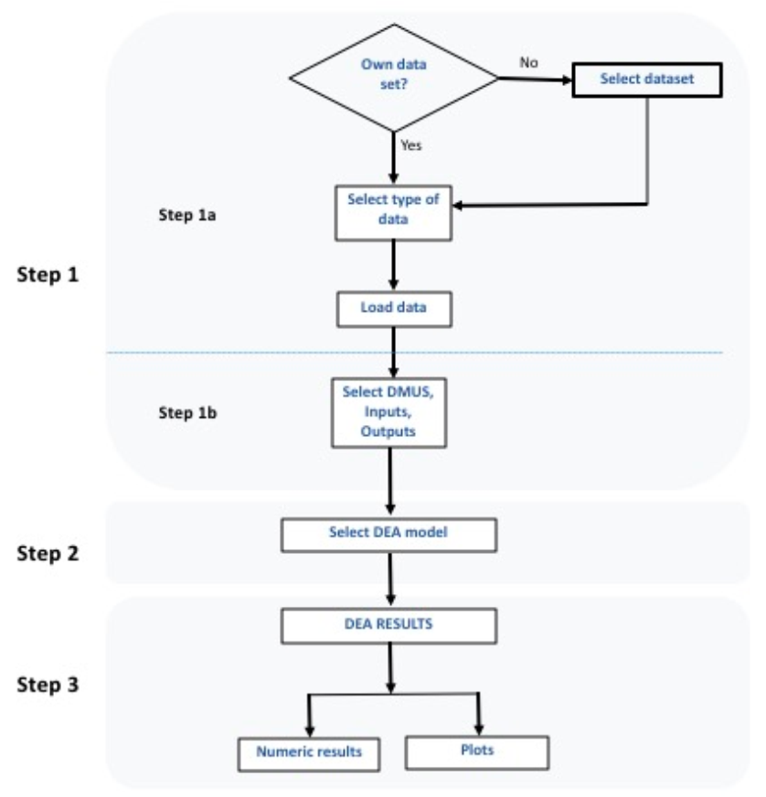
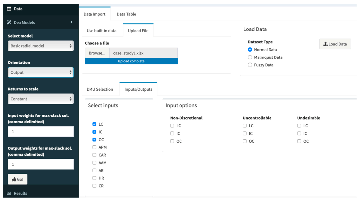
- Step 1 a: Loading data. Firstly, we can upload our own dataset (the app identifies the most common file extensions: txt, csv, tsv, xls, xlsx, sav, dta, xpt, etc.) or load a built-in dataset (deaR-shiny is not only oriented to research but also to teaching, so the application provides 24 built-in datasets from published articles). Once the data file is selected, we have to indicate the type of data we will work with, which depends on the analysis model to be applied. Thus, we will select the Normal Data option if a conventional DEA model is going to be executed, the Malmquist Data option to perform the Malmquist productivity index, or the Fuzzy Data option to run an FDEA model with uncertain data.To reproduce the results given in [76], we need to click on the Upload file tab and then on the button Browse to select the Excel file (case_study1.xlsx). As the option Normal Data is selected by default, we only have to click on the button Load Data to load the dataset. We should see something similar as Figure 3.To take a quick glimpse at the uploaded data, we click on the Data table Table In doing this, we can see that Comiso Airport has three missing values.
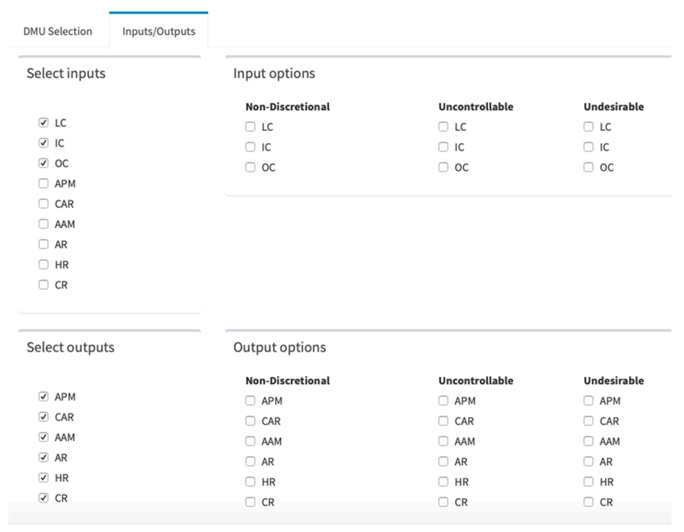
- Step 1 b: Selecting variables. Once the dataset is loaded, deaR-shiny automatically reads it and identifies the names of the header as the names of the variables. By default, the application considers that the DMUs are in the first column (if it is not, we can select the correct DMU column by pulling down the menu) and the rest of the columns are the inputs/outputs.At this point, all the DMUs are selected for evaluation. Alternatively, we can select the DMUs that will constitute the evaluation reference set (DMU ref) and the DMUs to be evaluated (DMU eval). As Comiso Airport has missing values and we do not know how [76] treated them, we will omit this DMU. Therefore, we deselect Comiso from both DMU eval and DMU ref.In addition, as Figure 4 shows, we also must identify which variables are inputs and which are outputs. This is done in the tab Inputs/Outputs. To measure the efficiency of regional Italian airports, [76] use three inputs (LC, IC, and OC) and six outputs (APM, CAR, AAM, AR, HR, and CR). To select them, we click on the corresponding check box. Note that we could also indicate whether there are uncontrollable, non-discretionary or undesirable inputs/outputs.
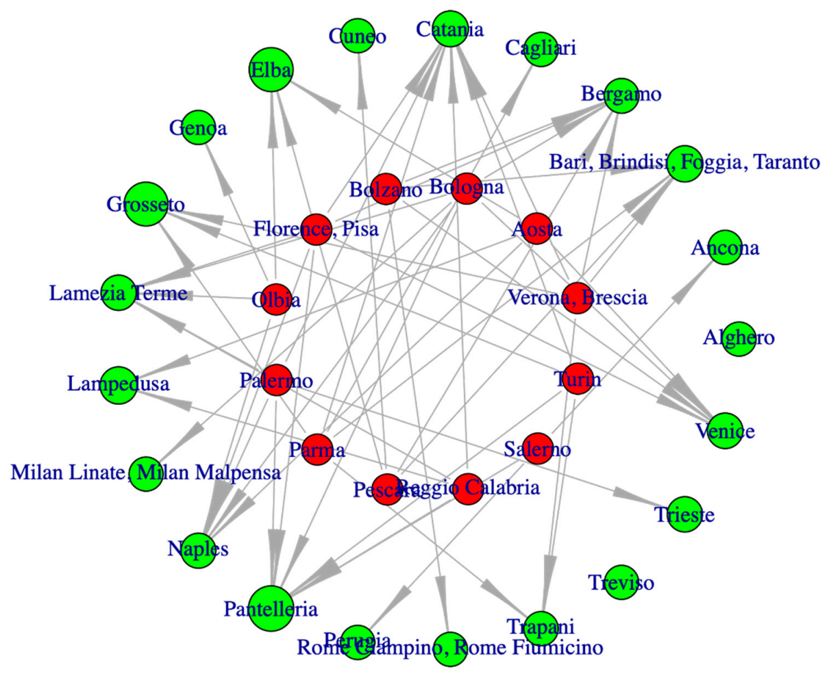
- In the left panel, the different types of results, organized in tabs, are shown in a table. In general, the numeric results offered by deaR-shiny refer to efficiency scores, slacks, target values, intensities (lambdas) or multipliers, and the reference set for inefficient DMUs. However, the results shown depend on the model executed. For example, if we run the Malmquist index, the results provided by deaR-shiny will be related to total factor productivity change, technical efficiency change (under CRS), pure technical efficiency change (under VRS), scale efficiency change, and technological change.Three action buttons are also provided in the left panel: Copy, Print and Download (to download the results in csv, pdf or excel format).
- In the right panel are some options for saving the results. Thus, we can select the results to be exported as well as give a name and extension format to the file. deaR-shiny gives the name ResultsDEAyear-month-day_hour:minute:second.xlsx by default. To save the results, we click on the button Create Excel file and then on Download excel file.
3.2. Case Study 2. Kao and Liu (2000, 2003)
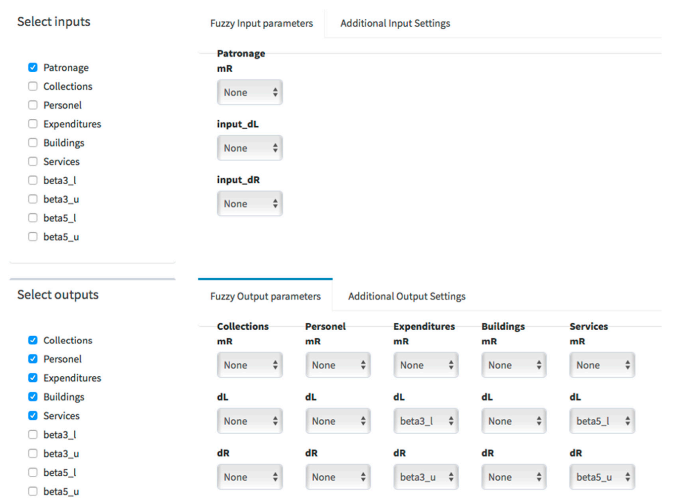
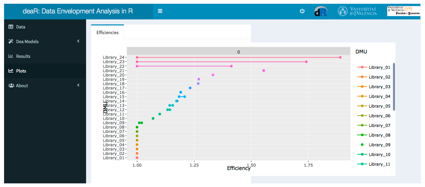
- Patronage: It is a weighted sum of the standardized scores of faculty, graduate students, undergraduate students, and extension students.
- Collections: Books, serials, microforms, audiovisual works, and database.
- Personnel: Classified staff, unclassified staff, and student assistants.
- Expenditures: Capital expenditure, operating expenditure, and special expenditure.
- Buildings: Area and seats.
- Services: Operating hours, attendance, circulation, communication channels, range of services, amount of services, etc.
4. Conclusions
Supplementary Materials
Author Contributions
Funding
Institutional Review Board Statement
Informed Consent Statement
Data Availability Statement
Conflicts of Interest
References
- Seiford, L.M. A bibliography for Data Envelopment Analysis (1978–1996). Ann. Oper. Res. 1997, 73, 393–438. [Google Scholar] [CrossRef]
- Tavares, G. A Bibliography of Data Envelopment Analysis (1978–2001); RUTCOR; Rutgers University: New Brunswick, NJ, USA, 2002. [Google Scholar]
- Emrouznejad, A.; Parker, B.R.; Tavares, G. Evaluation of research in efficiency and productivity: A survey and analysis of the first 30 years of scholarly literature in DEA. Socioecon. Plann. Sci. 2008, 42, 151–157. [Google Scholar] [CrossRef]
- Cook, W.D.; Seiford, L.M. Data envelopment analysis (DEA)—Thirty years on. Eur. J. Oper. Res. 2009, 192, 1–17. [Google Scholar] [CrossRef]
- Emrouznejad, A.; Yang, G. A survey and analysis of the first 40 years of scholarly literature in DEA: 1978–2016. Socioecon. Plann. Sci. 2018, 61, 4–8. [Google Scholar] [CrossRef]
- Zhou, H.; Yang, Y.; Chen, Y.; Zhu, J. Data envelopment analysis application in sustainability: The origins, development and future directions. Eur. J. Oper. Res. 2018, 264, 1–16. [Google Scholar] [CrossRef]
- Charnes, A.; Cooper, W.W.; Rhodes, E. Measuring the efficiency of decision making units. Eur. J. Oper. Res. 1978, 2, 429–444. [Google Scholar] [CrossRef]
- Banker, R.D.; Charnes, A.; Cooper, W.W. Some Models for Estimating Technical and Scale Inefficiencies in Data Envelopment Analysis. Manage. Sci. 1984, 30, 1078–1092. [Google Scholar] [CrossRef]
- Banker, R.D.; Morey, R.C. Efficiency Analysis for Exogenously Fixed Inputs and Outputs. Oper. Res. 1986, 34, 513–521. [Google Scholar] [CrossRef]
- Banker, R.D.; Morey, R.C. The Use of Categorical Variables in Data Envelopment Analysis. Manag. Sci. 1986, 32, 1613–1627. [Google Scholar] [CrossRef]
- Cook, W.D.; Kress, M.; Seiford, L.M. On the Use of Ordinal Data in Data Envelopment Analysis. J. Oper. Res. Soc. 1993, 44, 133–140. [Google Scholar] [CrossRef]
- Thompson, R.G.; Singleton, F.D.; Thrall, R.M.; Smith, B.A. Comparative Site Evaluations for Locating a High-Energy Physics Lab in Texas. Interfaces 1986, 16, 35–49. [Google Scholar] [CrossRef]
- Thompson, R.G.; Langemeier, L.N.; Lee, C.T.; Lee, E.; Thrall, R.M. The role of multiplier bounds in efficiency analysis with application to Kansas farming. J. Econom. 1990, 46, 93–108. [Google Scholar] [CrossRef]
- Charnes, A.; Cooper, W.W.; Wei, Q.L.; Huang, Z.M. Cone ratio data envelopment analysis and multi-objective programming. Int. J. Syst. Sci. 1989, 20, 1099–1118. [Google Scholar] [CrossRef]
- Charnes, A.; Cooper, W.W.; Huang, Z.M.; Sun, D.B. Polyhedral Cone-Ratio DEA Models with an illustrative application to large commercial banks. J. Econom. 1990, 46, 73–91. [Google Scholar] [CrossRef]
- Dyson, R.G.; Thanassoulis, E. Reducing Weight Flexibility in Data Envelopment Analysis. J. Oper. Res. Soc. 1988, 39, 563–576. [Google Scholar] [CrossRef]
- Seiford, L.M.; Zhu, J. Modeling undesirable factors in efficiency evaluation. Eur. J. Oper. Res. 2002, 142, 16–20. [Google Scholar] [CrossRef]
- Färe, R.; Grosskopf, S.; Lovell, C.A.K.; Pasurka, C. Multilateral Productivity Comparisons When Some Outputs are Undesirable: A Nonparametric Approach. Rev. Econ. Stat. 1989, 71, 90–98. [Google Scholar] [CrossRef]
- Charnes, A.; Cooper, W.W.; Golany, B.; Seiford, L.; Stutz, J. Foundations of data envelopment analysis for Pareto-Koopmans efficient empirical production functions. J. Econom. 1985, 30, 91–107. [Google Scholar] [CrossRef]
- Thanassoulis, E.; Portela, M.C.S.; Despić, O. DEA—The Mathematical Programming Approach to Efficiency Analysis. In The Measurement of Productive Efficiency and Productivity Change; Fried, H.O., Knox Lovell, C.A., Schmidt, S.D., Eds.; Oxford Scholarship: Oxford, UK, 2008; pp. 1–161. ISBN 9780195183528. [Google Scholar]
- Tone, K. A slacks-based measure of efficiency in data envelopment analysis. Eur. J. Oper. Res. 2001, 130, 498–509. [Google Scholar] [CrossRef]
- Fare, R.; Lovell, C. Measuring the technical efficiency of production. J. Econ. Theory 1978, 19, 150–162. [Google Scholar] [CrossRef]
- Färe, R.; Grosskopf, S.; Knox Lovell, C.A. The Measurement of Efficiency and Production; Kluwer-Nijhoff: Boston, MA, USA, 1985; ISBN 9789048158133. [Google Scholar]
- Pastor, J.T.; Ruiz, J.L.; Sirvent, I. An enhanced DEA Russell graph efficiency measure. Eur. J. Oper. Res. 1999, 115, 596–607. [Google Scholar] [CrossRef]
- Zhu, J. Data envelopment analysis with preference structure. J. Oper. Res. Soc. 1996, 47, 136–150. [Google Scholar] [CrossRef]
- Cooper, W.W.; Park, K.S.; Pastor, J.T. RAM: A Range Adjusted Measure of Inefficiency for Use with Additive Models, and Relations to Other Models and Measures in DEA. J. Product. Anal. 1999, 11, 5–42. [Google Scholar] [CrossRef]
- Adler, N.; Friedman, L.; Sinuany-Stern, Z. Review of ranking methods in the data envelopment analysis context. Eur. J. Oper. Res. 2002, 140, 249–265. [Google Scholar] [CrossRef]
- Andersen, P.; Petersen, N.C. A Procedure for Ranking Efficient Units in Data Envelopment Analysis. Manage. Sci. 1993, 39, 1261–1264. [Google Scholar] [CrossRef]
- Tone, K. A slacks-based measure of super-efficiency in data envelopment analysis. Eur. J. Oper. Res. 2002, 143, 32–41. [Google Scholar] [CrossRef]
- Du, J.; Liang, L.; Zhu, J. A slacks-based measure of super-efficiency in data envelopment analysis: A comment. Eur. J. Oper. Res. 2010, 204, 694–697. [Google Scholar] [CrossRef]
- Sexton, T.R.; Silkman, R.H.; Hogan, A.J. Data envelopment analysis: Critique and extensions. New Dir. Progr. Eval. 1986, 1986, 73–105. [Google Scholar] [CrossRef]
- Doyle, J.; Green, R. Efficiency and Cross-efficiency in DEA: Derivations, Meanings and Uses. J. Oper. Res. Soc. 1994, 45, 567–578. [Google Scholar] [CrossRef]
- Caves, D.W.; Christensen, L.R.; Diewert, W. The Economic Theory of Index Numbers and the Measurement of Input, Output, and Productivity. Econometrica 1982, 50, 1393–1414. [Google Scholar] [CrossRef]
- Fare, R.; Grosskopf, S.; Norris, M.; Zhang, Z. Productivity Growth, Technical Progress, and Efficiency Change in Industrialized Countries. Am. Econ. Rev. 1994, 84, 66–83. [Google Scholar]
- Ray, S.C.; Desli, E. Productivity Growth, Technical Progress, and Efficiency Change in Industrialized Countries: Comment. Am. Econ. Rev. 1997, 87, 1033–1039. [Google Scholar]
- Grifell-Tatjé, E.; Lovell, C.A.K. A generalized Malmquist productivity index. Top 1999, 7, 81–101. [Google Scholar] [CrossRef]
- Shestalova, V. Sequential Malmquist Indices of Productivity Growth: An Application to OECD Industrial Activities. J. Product. Anal. 2003, 19, 211–226. [Google Scholar] [CrossRef]
- Pastor, J.T.; Lovell, C.A.K. A global Malmquist productivity index. Econ. Lett. 2005, 88, 266–271. [Google Scholar] [CrossRef]
- Charnes, A.; Clark, C.T.; Cooper, W.W.; Golany, B. A developmental study of data envelopment analysis in measuring the efficiency of maintenance units in the U.S. air forces. Ann. Oper. Res. 1984, 2, 95–112. [Google Scholar] [CrossRef]
- Simar, L.; Wilson, P.W. Sensitivity analysis of efficiency scores: How to bootstrap in nonparametric frontier models. Manage. Sci. 1998, 44, 49–61. [Google Scholar] [CrossRef]
- Löthgren, M. How to Bootstrap DEA Estimators: A Monte Carlo Comparison; SSE/EFI Working Paper Series in Economics and Finance; Stockholm School of Economics: Stockholm, Sweden, 1998. [Google Scholar]
- Löthgren, M.; Tambour, M. Bootstrapping the data envelopment analysis Malmquist productivity index. Appl. Econ. 1999, 31, 417–425. [Google Scholar] [CrossRef]
- Simar, L.; Wilson, P.W. Statistical Inference in Nonparametric Frontier Models: The State of the Art. J. Product. Anal. 2000, 13, 49–78. [Google Scholar] [CrossRef]
- Cooper, W.W.; Deng, H.; Huang, Z.; Li, S.X. Chance constrained programming approaches to technical efficiencies and inefficiencies in stochastic data envelopment analysis. J. Oper. Res. Soc. 2002, 53, 1347–1356. [Google Scholar] [CrossRef]
- Ray, S.C. Data Envelopment Analysis. Theory and Techniques for Economics and Operations Research; Cambridge University Press: New York, NY, USA, 2004. [Google Scholar]
- Olesen, O.B.; Petersen, N.C. Stochastic data envelopment analysis—A review. Eur. J. Oper. Res. 2016, 251, 2–21. [Google Scholar] [CrossRef]
- Hatami-Marbini, A.; Emrouznejad, A.; Tavana, M. A taxonomy and review of the fuzzy data envelopment analysis literature: Two decades in the making. Eur. J. Oper. Res. 2011, 214, 457–472. [Google Scholar] [CrossRef]
- Zhou, W.; Xu, Z. An Overview of the Fuzzy Data Envelopment Analysis Research and Its Successful Applications. Int. J. Fuzzy Syst. 2020, 22, 1037–1055. [Google Scholar] [CrossRef]
- Barr, R.S. DEA software tools and technology. A State-of-the-Art Survey. In Handbook on Data Envelopment Analysis; Cooper, W.W., Seiford, L.M., Zhu, J., Eds.; Springer: Boston, MA, USA, 2004; pp. 539–566. [Google Scholar]
- Cooper, W.W.; Seiford, L.M.; Tone, K. Data Envelopment Analysis: A Comprehensive Text with Models, Applications, References and DEA-Solver Software, 2nd ed.; Springer: Boston, MA, USA, 2007. [Google Scholar]
- Daraio, C.; Kerstens, K.H.J.; Nepomuceno, T.C.C.; Sickles, R. Productivity and Efficiency Analysis Software: An Exploratory Bibliographical Survey of the Options. J. Econ. Surv. 2019, 33, 85–100. [Google Scholar] [CrossRef]
- Ji, Y.; Lee, C. Data envelopment analysis. Stata J. 2010, 10, 267–280. [Google Scholar] [CrossRef]
- Álvarez, I.C.; Barbero, J.; Zofío, J.L. A Data Envelopment Analysis Toolbox for MATLAB. J. Stat. Softw. 2020, 95, 1–49. [Google Scholar] [CrossRef]
- R Core Team. R: A Language and Environment for Statistical Computing; R Foundation for Statistical Computing: Vienna, Austria, 2021; Available online: https://www.R-project.org/ (accessed on 14 June 2021).
- Wilson, P.W. FEAR: A software package for frontier efficiency analysis with R. Socioecon. Plann. Sci. 2008, 42, 247–254. [Google Scholar] [CrossRef]
- Bogetoft, P.; Otto, L. Benchmarking with DEA, SFA, and R; Springer: New York, NY, USA, 2011; ISBN 978-1-4419-7960-5. [Google Scholar]
- Oh, D.; Suh, D. nonparaeff: Nonparametric Methods for Measuring Efficiency and Productivity. R package version 0.5-5. 2013. Available online: https://CRAN.R-project.org/package=nonparaeff (accessed on 14 June 2021).
- Simm, J.; Besstremyannaya, G. rDEA: Robust Data Envelopment Analysis (DEA) for R. R package version 1.2-6. 2020. Available online: https://CRAN.R-project.org/package=rDEA (accessed on 14 June 2021).
- Lim, D. DJL: Distance Measure Based Judgment and Learning. R package version 3.7. 2020. Available online: https://CRAN.R-project.org/package=DJL (accessed on 14 June 2021).
- Coll-Serrano, V.; Bolós, V.; Benítez Suárez, R. deaR: Conventional and Fuzzy Data Envelopment Analysis. R package version 1.2.3. 2021. Available online: https://CRAN.R-project.org/package=deaR (accessed on 14 June 2021).
- Coll-Serrano, V.; Benítez, R.; Bolós, V. Data Envelopment Analysis with deaR. 2018, pp. 1–48. Available online: https://www.uv.es/deaRshiny/deaR.html (accessed on 14 June 2021).
- Aparicio, J.; Ortiz, L.; Pastor, J.T. Design and implementation of a shiny interactive web application by rstudio for estimating Data Envelopment Analysis efficiency measures. Bol. Estad. e Investig. Oper. 2018, 34, 25–50. [Google Scholar]
- Pastor, J.T.; Lovell, C.A.K.; Aparicio, J. Families of linear efficiency programs based on Debreu’s loss function. J. Product. Anal. 2012, 38, 109–120. [Google Scholar] [CrossRef]
- Chang, W.; Cheng, J.; Allaire, J.; Xie, Y.; MacPherson, J. Shiny: Web Application Framework for R. R package version 1.6.0. 2021. Available online: https://CRAN.R-project.org/package=shiny (accessed on 14 June 2021).
- Chang, W.; Borges Ribeiro, B. shinydashboard: Create Dashboards with “Shiny”. R package version 0.7.1. 2018. Available online: https://CRAN.R-project.org/package=shinydashboard (accessed on 14 June 2021).
- Chambers, R.G.; Chung, Y.; Färe, R. Benefit and Distance Functions. J. Econ. Theory 1996, 70, 407–419. [Google Scholar] [CrossRef]
- Chambers, R.G.; Chung, Y.; Färe, R. Profit, Directional Distance Functions, and Nerlovian Efficiency. J. Optim. Theory Appl. 1998, 98, 351–364. [Google Scholar] [CrossRef]
- Kao, C.; Liu, S.T. Fuzzy efficiency measures in data envelopment analysis. Fuzzy Sets Syst. 2000, 113, 427–437. [Google Scholar] [CrossRef]
- Guo, P.; Tanaka, H. Fuzzy DEA: A perceptual evaluation method. Fuzzy Sets Syst. 2001, 119, 149–160. [Google Scholar] [CrossRef]
- León, T.; Liern, V.; Ruiz, J.L.; Sirvent, I. A fuzzy mathematical programming approach to the assessment of efficiency with DEA models. Fuzzy Sets Syst. 2003, 139, 407–419. [Google Scholar] [CrossRef]
- Sirvent, I.; León, T. Cross-Efficiency in Fuzzy Data Envelopment Analysis (FDEA): Some Proposals. In Performance Measurement with Fuzzy Data Envelopment Analysis. Studies in Fuzziness and Soft Computing; Emrouznejad, A., Tavana, M., Eds.; Springer: Berlin/Heidelberg, Germany, 2004; ISBN 978-3-642-41371-1. [Google Scholar]
- Coelli, T.J.; Prasada Rao, D.S.; Battesse, G.E. An Introduction to Efficiency and Productivity Analysis; Kluwer Academic Publishers: Boston, MA, USA, 1998. [Google Scholar]
- Deprins, D.; Simar, L.; Tulkens, H. Measuring Labor-Efficiency in Post Offices; CORE Discussion Papers RP; Université catholique de Louvain, Center for Operations Research and Econometrics (CORE): Louvain, Belgium, 1984. [Google Scholar]
- Thrall, R.M. What Is the Economic Meaning of FDH? J. Product. Anal. 1999, 11, 243–250. [Google Scholar] [CrossRef]
- Portela, M.C.A.S.; Thanassoulis, E.; Simpson, G. Negative data in DEA: A directional distance approach applied to bank branches. J. Oper. Res. Soc. 2004, 55, 1111–1121. [Google Scholar] [CrossRef]
- Carlucci, F.; Cirà, A.; Coccorese, P. Measuring and explaining airport efficiency and sustainability: Evidence from Italy. Sustainability 2018, 10, 400. [Google Scholar] [CrossRef]
- Kao, C.; Liu, S.T. A mathematical programming approach to fuzzy efficiency ranking. Int. J. Prod. Econ. 2003, 86, 145–154. [Google Scholar] [CrossRef]
- Kao, C.; Liu, S.-T. Data Envelopment Analysis with Missing Data: An Application to University Libraries in Taiwan. J. Oper. Res. Soc. 2000, 51, 897–905. [Google Scholar] [CrossRef]




| Model | deaR Function Name | References |
|---|---|---|
| Basic radial models | ||
| CCR | model_basic | [7] |
| BCC | model_basic | [8] |
| Multiplier | model_multiplier | [7] |
| Directional function | model_basic | [66,67] |
| Non-radial models | ||
| Additive | model_additive | [19,26] |
| Non-radial | model_nonradial | [22,23,24] |
| Preference structure | model_deaps | [25] |
| SBM efficiency | model_sbmeff | [21] |
| Super-efficiency models | ||
| Radial super-efficiency | model_supereff | [28] |
| SBM super-efficiency | model_sbmsupereff | [29] |
| Additive super-efficiency | model_addsupereff | [30] |
| Fuzzy models | ||
| Kao–Liu models | modelfuzzy_kaoliu | [68] |
| Guo–Tanaka model | modelfuzzy_guotanaka | [69] |
| Possibilistic model | modelfuzzy_possibilistic | [70] |
| Fuzzy cross-efficiency | cross_efficiency_fuzzy | [71] |
| Other models | ||
| Profit model | model_profit | [72] |
| Free disposal hull | model_fdh | [73,74] |
| Cross-efficiency | cross_efficiency | [31,32] |
| Malmquist index | malmquist_index | [33,34,35,36,37,38] |
| DMUs | 2 Inputs–2 Outputs | 3 Inputs–3 Outputs | 4 Inputs–4 Outputs | 5 Inputs–5 Outputs |
|---|---|---|---|---|
| 100 | 0.27 | 0.29 | 0.30 | 0.33 |
| 500 | 1.74 | 2.03 | 2.26 | 2.65 |
| 1000 | 5.06 | 6.20 | 7.10 | 8.55 |
| 2000 | 21.14 | 26.62 | 28.89 | 29.11 |
| 5000 | 91.8 | 153 | 178.2 | 224.4 |
| No. | Airports | LC | IC | OC | APM | CAR | AAM | AR | HR | CR |
|---|---|---|---|---|---|---|---|---|---|---|
| 1 | Alghero | 8,025,864 | 36,052,732 | 13,677,810 | 1,443,013 | 2226 | 12,866 | 9,613,708 | 6,409,138 | 6,473,765 |
| 2 | Ancona | 4,049,976 | 39,608,618 | 10554594 | 495,208 | 6331 | 11,719 | 2,567,103 | 1,711,402 | 6,530,518 |
| 3 | Aosta | 1,094,952 | 9,722,395 | 2056300 | 1863 | 0 | 147 | 1,160,011 | 77,334 | 282,409 |
| 4 | Bari, Brindisi, Foggia, Taranto | 16,420,571 | 321,136,731 | 54,919,104 | 4,952,786 | 5835 | 47,428 | 31,928,605 | 21,285,736 | 28,181,155 |
| 5 | Bergamo | 20,855,345 | 168,863,971 | 63,098,381 | 7,498,016 | 118,846 | 66,881 | 59,666,133 | 39,777,422 | 5,950,929 |
| 6 | Bologna | 19,155,505 | 204,834,129 | 40,858,309 | 5,580,005 | 28,973 | 61,337 | 45,083,791 | 30,055,861 | 1,640,828 |
| 7 | Bolzano | 1,294,115 | 24,026,015 | 3,912,906 | 4719 | 0 | 2193 | 2,768,064 | 1,845,375 | 1,085,631 |
| 8 | Cagliari | 5,698,746 | 131,131,392 | 27,463,390 | 3,334,477 | 3729 | 31,878 | 5,641,924 | 3,761,282 | 113,338 |
| 9 | Catania | 12,842,151 | 127,452,805 | 33,661,739 | 6,449,803 | 7721 | 56,603 | 34,367,013 | 22,911,342 | 2,465,137 |
| 10 | Comiso | 63,154 | 19,381,025 | 2,038,015 | 304,144 | 1 | 2176 | |||
| 11 | Cuneo | 1,208,104 | 8,462,489 | 4,727,013 | 16,668 | 686 | 1871 | 2,772,736 | 1,848,490 | 815,392 |
| 12 | Elba | 352,581 | 3,355,756 | 597,399 | 12,211 | 0 | 764 | 349,462 | 232,975 | 569,368 |
| 13 | Florence, Pisa | 23,920,438 | 130,935,629 | 41,453,079 | 6,197,995 | 7929 | 67,199 | 41,476,200 | 27,650,800 | 1,444,333 |
| 14 | Genoa | 11,375,395 | 20,766,869 | 11,843,283 | 1,242,709 | 849 | 16,227 | 13,367,713 | 8,911,809 | 1,832,522 |
| 15 | Grosseto | 153,468 | 3,697,845 | 343,922 | 3975 | 0 | 1764 | 320,292 | 213,528 | 38,459 |
| 16 | Lamezia Terme | 10,501,380 | 28,881,847 | 10,473,308 | 1,976,029 | 1750 | 16,364 | 13,414,410 | 8,942,940 | 1,165,734 |
| 17 | Lampedusa | 1,329,054 | 2,552,140 | 766,069 | 192,356 | 29 | 3548 | 1,400,025 | 93,335 | 59 |
| 18 | Milan Linate, Milan Malpensa | 147,076,237 | 1,492,519,434 | 292,537,314 | 28,453,800 | 467,073 | 28,607 | 345,320,721 | 230,213,814 | 22,333,333 |
| 19 | Naples | 17,286,071 | 111,631,557 | 37,211,266 | 5,714,451 | 5143 | 54,995 | 44,559,699 | 29,706,466 | 1,732,137 |
| 20 | Olbia | 10,829,469 | 50,440,841 | 15,045,089 | 1,901,930 | 452 | 19,964 | 16,784,081 | 11,189,387 | 3,503,293 |
| 21 | Palermo | 15,828,236 | 101,536,608 | 33,567,418 | 4,590,243 | 2623 | 44,932 | 28,895,596 | 19,263,730 | 3,507,620 |
| 22 | Pantelleria | 883,887 | 1,759,243 | 743,175 | 139,359 | 57 | 3965 | 941,855 | 627,903 | 3982 |
| 23 | Parma | 1,270,366 | 24,531,039 | 5,367,039 | 205,617 | 158 | 3732 | 1,067,534 | 711,689 | 349,086 |
| 24 | Perugia | 1,774,005 | 7,130,874 | 2,550,339 | 16,483 | 10 | 3148 | 1,261,548 | 841,032 | 1,618,795 |
| 25 | Pescara | 2,418,650 | 25,141,532 | 7,798,159 | 482,548 | 1566 | 6265 | 4,610,930 | 3,073,953 | 2,257,978 |
| 26 | Reggio Calabria | 2,889,940 | 24,331,288 | 4,280,518 | 515,081 | 135 | 5995 | 2,239,858 | 1,493,238 | 143,177 |
| 27 | Rome, Ciampino, Rome, Fiumicino | 97,201,545 | 2,730,020,455 | 429,363,545 | 41,019,736 | 16,927 | 363,707 | 400,779,800 | 267,186,533 | 19,479,666 |
| 28 | Salerno | 1,189,313 | 3,190,573 | 1,606,269 | 7713 | 0 | 978 | 177,558 | 118,372 | 38,413 |
| 29 | Turin | 12,315,576 | 134,879,749 | 37,571,120 | 3,475,463 | 1639 | 42,486 | 6,447,551 | 4,298,367 | 1,999,882 |
| 30 | Trapani | 3,301,846 | 31,779,539 | 8,419,712 | 1,245,434 | 325 | 14,853 | 5,787,979 | 3,858,653 | 2,819,165 |
| 31 | Treviso | 5,106,233 | 37,278,326 | 14,540,126 | 1,926,415 | 5797 | 14,792 | 12,140,877 | 8,093,918 | 737,758 |
| 32 | Trieste | 5,587,525 | 14,749,260 | 9,569,079 | 761,813 | 198 | 11,259 | 7,929,407 | 5,286,271 | 3,020,194 |
| 33 | Venice | 22,076,250 | 418,140,375 | 53,564,125 | 7,747,417 | 28,738 | 78,398 | 65,964,400 | 43,976,266 | 62,933,33 |
| 34 | Verona, Brescia | 10,517,572 | 120,563,482 | 35,169,083 | 3,103,782 | 18,732 | 33,646 | 21,392,893 | 14,261,928 | 3,807,184 |
| No. | Airports | Output-Oriented CRS | Output-Oriented VRS |
|---|---|---|---|
| 1 | Alghero | 1.00 | 1.00 |
| 2 | Ancona | 1.00 | 1.00 |
| 3 | Aosta | 1.94 | 1.93 |
| 4 | Bari, Brindisi, Foggia, Taranto | 1.00 | 1.00 |
| 5 | Bergamo | 1.00 | 1.00 |
| 6 | Bologna | 1.05 | 1.00 |
| 7 | Bolzano | 1.17 | 1.17 |
| 8 | Cagliari | 1.00 | 1.00 |
| 9 | Catania | 1.00 | 1.00 |
| 10 | Comiso 1 | ||
| 11 | Cuneo | 1.00 | 1.00 |
| 12 | Elba | 1.00 | 1.00 |
| 13 | Florence, Pisa | 1.15 | 1.00 |
| 14 | Genoa | 1.00 | 1.00 |
| 15 | Grosseto | 1.00 | 1.00 |
| 16 | Lamezia Terme | 1.00 | 1.00 |
| 17 | Lampedusa | 1.00 | 1.00 |
| 18 | Milan Linate, Milan Malpensa | 1.00 | 1.00 |
| 19 | Naples | 1.00 | 1.00 |
| 20 | Olbia | 1.01 | 1.00 |
| 21 | Palermo | 1.15 | 1.04 |
| 22 | Pantelleria | 1.00 | 1.00 |
| 23 | Parma | 2.12 | 1.86 |
| 24 | Perugia | 1.00 | 1.00 |
| 25 | Pescara | 1.07 | 1.05 |
| 26 | Reggio Calabria | 1.68 | 1.60 |
| 27 | Rome, Ciampino, Rome, Fiumicino | 1.00 | 1.00 |
| 28 | Salerno | 5.17 | 4.75 |
| 29 | Turin | 1.50 | 1.28 |
| 30 | Trapani | 1.00 | 1.00 |
| 31 | Treviso | 1.00 | 1.00 |
| 32 | Trieste | 1.00 | 1.00 |
| 33 | Venice | 1.00 | 1.00 |
| 34 | Verona, Brescia | 1.28 | 1.23 |
| Inefficient Airport | ||||||||||||
|---|---|---|---|---|---|---|---|---|---|---|---|---|
| Efficient Airport | Aosta | Bologna | Bolzano | Florence Pisa | Olbia | Palermo | Parma | Pescara | Reggio Calabria | Salerno | Turin | Verona Brescia |
| Ancona | 0.023 | |||||||||||
| Bari Brindisi Foggia Taranto | 0.039 | 0.000 | 0.017 | 0.023 | 0.096 | |||||||
| Bergamo | 0.165 | 0.006 | 0.021 | 0.055 | 0.223 | |||||||
| Cagliari | 0.062 | |||||||||||
| Catania | 0.389 | 0.562 | 0.012 | 0.098 | 0.725 | 0.283 | ||||||
| Cuneo | 0.021 | |||||||||||
| Elba | 0.778 | 4.626 | 2.489 | |||||||||
| Grosseto | 0.138 | 2.121 | 8.448 | 4.395 | ||||||||
| Lamezia Terme | 0.539 | 0.000 | 0.194 | |||||||||
| Lampedusa | 0.110 | 1.562 | 0.559 | 3.356 | 1.129 | |||||||
| Naples | 0.028 | 0.269 | 0.476 | 0.210 | 0.111 | |||||||
| Pantelleria | 1.826 | 4.363 | 0.591 | 0.144 | 1.186 | 0.771 | ||||||
| Perugia | 0.027 | |||||||||||
| Rome Ciampino Rome Fiumicino | 0.001 | |||||||||||
| Trapani | 0.047 | 0.312 | 0.001 | |||||||||
| Trieste | 0.199 | 0.740 | ||||||||||
| Venice | 0.009 | 0.333 | 0.021 | |||||||||
Publisher’s Note: MDPI stays neutral with regard to jurisdictional claims in published maps and institutional affiliations. |
© 2021 by the authors. Licensee MDPI, Basel, Switzerland. This article is an open access article distributed under the terms and conditions of the Creative Commons Attribution (CC BY) license (https://creativecommons.org/licenses/by/4.0/).
Share and Cite
Benítez, R.; Coll-Serrano, V.; Bolós, V.J. deaR-Shiny: An Interactive Web App for Data Envelopment Analysis. Sustainability 2021, 13, 6774. https://doi.org/10.3390/su13126774
Benítez R, Coll-Serrano V, Bolós VJ. deaR-Shiny: An Interactive Web App for Data Envelopment Analysis. Sustainability. 2021; 13(12):6774. https://doi.org/10.3390/su13126774
Chicago/Turabian StyleBenítez, Rafael, Vicente Coll-Serrano, and Vicente J. Bolós. 2021. "deaR-Shiny: An Interactive Web App for Data Envelopment Analysis" Sustainability 13, no. 12: 6774. https://doi.org/10.3390/su13126774
APA StyleBenítez, R., Coll-Serrano, V., & Bolós, V. J. (2021). deaR-Shiny: An Interactive Web App for Data Envelopment Analysis. Sustainability, 13(12), 6774. https://doi.org/10.3390/su13126774


