Selecting Suitable, Green Port Crane Equipment for International Commercial Ports

Abstract

Responding to the increasing global need for environmental protection, a green port balances economic vibrancy with environmental protection. However, because exhaust emissions (e.g., CO₂ or sulfide) are difficult to monitor around ports, data on such emissions are often incomplete, which hinders research on this topic. The present study aimed to fill this gap in this topic. To remedy this problem, this study formulated a new data envelopment analysis (DEA) method for collecting CO₂ emissions data at their source. This method was applied to collect real-world operating data from a large container-handling company in Taiwan. Specifically, we provide a real example using a novel green energy index to account for undesirable outputs. Our main objective was to formulate two methods that combine: (1) data envelopment analysis based on a modified slack-based measure, and (2) a multi-choice goal programming approach. The contributions of this paper included the finding that rubber-tired gantry cranes are the greenest and should be used in ports. Finally, our findings aid port managers in selecting port equipment that provides the best balance between environmental protection and profitability.

1. Introduction

Environmental degradation and resource overconsumption are serious global problems, whereas sustainable development benefits both a country and its economy. Human activity is responsible for both environmental protection and environmentally damaging economic growth. Correspondingly, although a country’s natural resources (e.g., air, water, soil, and minerals) enable its development, their overexploitation is bound to backfire eventually, leaving future generations with environmental problems, such as wildlife extinction and natural resource depletion.

Human overreliance on fossil fuels has resulted in climate change, which is disruptive at best and destructive at worst. Climate change has and will destroy marine ecosystems, melt glaciers, decimate the Amazon rainforest, and trigger large-scale human migration and conflict [1]. Sea levels will also rise due to climate change, and eroded coastal conditions, the release of inundated land, and the threat of submersion will be disastrous for island nations and low-lying coastal areas. This threat is especially serious given that half of the global population lives within 100 km of a coast [2] and that coastal regions tend to be wealthy.

In response, many coastal governments have begun formulating strategies for sustainable development. Ports are a crucial driver of economic growth, but they are also energy intensive and a source of pollution. To remedy this problem and to ensure sustainable development, the concept of a green port was formulated. The move toward green ports has made considerable progress in many developed countries, as reflected in the San Pedro Bay Clean Air Action Plan (jointly implemented by the Port of Los Angeles, California, and the Port of Long Beach, New York and New Jersey), the Clean Air Initiatives and Harbor Air Management Plan (jointly implemented by port authorities in New York and New Jersey), the Rijnmond Regional Air Quality Action Program (implemented by the Port of Rotterdam, The Netherlands), and the Green Port Guidelines (implemented by the Port of Sydney, Australia).

In the context of these developments, more scholarly attention has been paid to the rational utilization of port resources [3,4,5,6,7,8]. Studies have aimed to assist port managers in formulating feasible policies from a macroscopic perspective that accounts for scaling effects and the balance between economic vibrancy and environmental protection. However, these studies have not considered the sources of environmental damage in and around ports (e.g., sources of CO₂ emissions). In response to this gap in the literature, this study focused on the container-handling system, which is closely related to daily port operations. Even though CO₂ emissions are an important consideration among port authority and terminal operators, the literature on this topic is limited. In general, few studies have focused on evaluating the environmental performance of green ports, likely because port emissions data (pertaining to, for example, CO₂ or sulfide) are difficult to collect. The present study aimed to fill this gap.

Specifically, this real-world example study combined data envelopment analysis (DEA) and multi-choice goal programming (MCGP) to evaluate the green performance of four types of cranes that are commonly used in ports. The findings will aid port managers in making their port greener. The contributions of this paper include: (1) the modified super slack-based measure (SBM-DEA) model, which is presented to evaluate the overall crane equipment efficiency, (2) the MCGP model’s use in choosing crane equipment, and (3) the application of the proposed approaches to port operation in Taiwan, alongside the provision of some valuable suggestions.

The remaining parts of the paper are organized as follows: Section 2 reviews the literature on green ports. Section 3 introduces this study’s combination of DEA, based on the modified SBM, and the MCGP method that accounts for undesirable outputs. A real-world case example in Taiwan is presented in Section 4. Finally, Section 5 concludes the paper and discusses the managerial implications.

2. Literature Review

2.1. Green Ports

In general, green port construction involves aspects such as improving water quality, supervising air quality, ensuring noise control, managing waste and hazardous cargo, conducting environmental education and training, and maintaining biodiversity in the port area. Scholars have researched these aspects.

In analyzing the water circulation patterns in the port of Ensenada (one of Mexico’s most important ports), Espino et al. [9] suggested the use of a wave energy pumping system to gradually dilute the concentration of pollutants in the port area. Otene and Nnadi [10] focused on water quality indices and water quality conditions in the Port of Harcourt, Nigeria. Their study collected water samples from four key locations in the port and analyzed the water quality parameters using standard methods. Their findings indicated the poor state of environmental monitoring, thus aiding the port’s managers. Lee et al. [11] analyzed a comprehensive 2010–2011 data set on marine environmental trends, including those of water quality, along the coast of Busan New Port. Their findings aided port managers in monitoring the impact of projects on the offshore marine environment around the port. Bolognese et al. [12] noted that, in contrast to the many studies that have investigated the management of noise from transportation, few studies have investigated the management of noise from port operations. The authors investigated the North Tyrrhenian Sea Port by collecting data from monitoring systems, noise measurements, and citizen complaints. Their findings indicated a neglect of noise levels by port managers. Reviewing the regulations and literature on environmental issues in port management systems, Vaio et al. [13] conducted semi-structured interviews with users of an Italian port to explore how port management control systems assist port authorities in the decision-making process. To help port managers improve management efficiency during ship mooring, their study also assessed the efficiency of port waste management.

Focusing on official regulations, Prati et al. [14] investigated the air quality in the Port of Naples through two experiments. Measurements were made at 15 points within the port. In addition, a laboratory was established within the port area to take continuous measurements of pollutant concentrations, ambient parameters, particulate matter (PM) levels, and wind direction and intensity. Their findings indicated that ship emissions contributed the most to SO₂ concentrations as compared to the concentrations of other pollutants. Kontos et al. [15] focused on the impact of gas emissions from cruise ships and passenger vessels on air quality and human health risks in the area around the Port of Thessaloniki. They estimated the surface concentration of pollutants caused by passenger ship traffic using the CALPUFF dispersion models for 2013, and their study also forecast trends for future environmental conditions within the port area. Casazza et al. [16] used 3D modeling to achieve the effective regulation of air quality within a port area. Their study not only enabled air pollution monitoring in ports, but also provided a new methodology in support of local environmental management systems. Progiou et al. [17] demonstrated that navigation emissions from ships are an important component of the total emissions, whether of a port, port city, or country. Their study used atmospheric models to simulate the dispersion of air pollutants, and their findings indicated a significant increase in activity in the Port of Piraeus over the last decade, especially from merchant ships.

As evident in the preceding literature review, studies have typically monitored the environment around port areas through monitoring stations, thus gaining a macro-level understanding [18,19,20,21,22,23]. In this study, we classified research topics on green performance evaluation methods, and several representative publications are listed in

Table 1. Variables selection of the recent studies for the green performance evaluation.

References	Research Topics	Method	Inputs				Outputs
			Types of Crane Equipment	Working Times	Energy Cost	Energy Consumption	Working Capacity	CO2 Emission
Casazza et al. [16]	Sustainable urban port	3D monitoring		√	√			√
Dong et al. [24]	Green port	DEA	√		√		√	√
Aisha et al. [25]	Sustainable terminals	ε-constraint		√	√	√	√	√
Li et al. [26]	Sustainable electric vehicle	Genetic algorithm			√	√		√
Progiou et al. [17]	Port emissions	Simulation			√	√		√
Budiyanto et al. [23]	Container terminal	Case study	√			√		√
Current study	Green port crane	Modified SBM-DEA		√	√	√	√	√

.

Few studies have monitored greenhouse gas emissions at their source. The cranes in a port are one such source, as they emit greenhouse gases when continually loading and unloading cargo. Therefore, the construction of an effective evaluation approach for selecting environmentally friendly cranes is a research problem of practical importance, and it is this problem (and gap in the literature) that this study aimed to address.

2.2. DEA Applied in Green Ports

Among the many existing methods for evaluating performance, DEA is well known by many managers and researchers alike because of its unique advantages in processing multiple inputs and outputs. The conventional DEA model was first proposed by Charnes et al. [27] in 1978. It was based on linear programming, which is a quantitative method of evaluating the relative effectiveness of comparable units of the same type. As DEA became methodologically more sophisticated with time, it has developed into a new field that integrates operations research, management science, and mathematical economics. Subsequently, Banker et al. [28] extended the DEA model to cover variable returns to scale (VRS). Since then, DEA models have been extended to other practical domains in the form of super-efficiency models [29,30,31], cross-efficiency models [32,33], SBM models [34,35], super-SBM models [36,37], and network DEA models [38,39,40].

Although DEA methods have often been used to evaluate performance with respect to CO₂ emissions [41,42,43,44,45,46], few have applied DEA to green ports specifically. Using an inseparable input–output SBM-DEA model, Na et al. [35] analyzed how environmentally friendly eight major container ports in China were by using 2005–2014 environmental monitoring data. Their results indicated that the eight ports significantly differed in their CO₂ emission levels and that their pure technical environmental efficiency was low. Li et al. [45] noted that the rapid development of China’s port industry has led to serious problems with CO₂ emissions. Specifically, the authors analyzed 2013–2018 data on 16 Chinese port companies; the ports were segmented by size and complexity criteria in the analysis. Using an improved non-radial directional distance function, they determined the performance of these ports with respect to CO₂ emissions. Wang et al. [46] constructed three DEA models to evaluate the environmental efficiency gained by cooperation between ports under the conditions of environmental control, non-environmental control, and PM emissions. They collected and analyzed data from 11 major Chinese ports and found that ports in the eastern region of China performed the best with respect to environmental friendliness.

3. Methodology

In the present study, a two method data envelopment analysis, based on a modified slack-based measure and a multi-choice goal programming approach, was used to evaluate the performance of green port crane equipment.

3.1. Modified SBM-DEA Model

The modified SBM-DEA model is described via the sets of indices, variables, and parameters presented in

Table 2. Nomenclature.

Index	$j=1,\dots ,n$	DMU (port crane equipment)
	$i=1,\dots ,m$	Inputs
	$r=1,\dots ,s$	Good outputs
	$h=1,\dots ,g$	Undesirable outputs
Variables	${\lambda }_j$	Weights of peers (DMU- j)
	$x_{ij}$	Input i of DMU- j
	$y_{rj}$	Output r of DMU- j
	$u_{hj}$	Undesirable output h of DMU- j
	$w_i^{-}$	Under achievement of input target i
	$w_r^{+}$	Over achievement of output target r
	$w_h^{-}$	Under achievement of undesirable output target h
	$s_i^{+}$	Extra slacks of input target i
	$s_r^{-}$	Extra slacks of output target r
	$s_h^{+}$	Extra slacks of undesirable output target h
Parameters	${\varphi }_j^{*}$	Super-efficiency of DMU- j
	$E_{\max }$	Maximum value of ${\varphi }_j$
	GIj	Green energy index of DMU- j

.

Suppose that n, decision-making units (DMUs), have m inputs and s outputs to be evaluated. Let $x_{ij}(i=1,\dots ,m)$, and $y_{rj}(r=1,\dots ,s)$ denote the ith input and rth output, respectively, of the jth DMU$(j=1,\dots ,n)$. The production possible set (PPS) given by the DMUs is as follows:

$$T=\left\{(x_1,\dots ,x_i,\dots ,x_m,y_1,\dots ,y_r,\dots ,y_s)|{\displaystyle \sum _{i=1}^m{v}_i{x}_{ij}}\le x_{ik},i=1,\dots ,m;{\displaystyle \sum _{i=1}^m{u}_r{y}_{rj}}\ge y_{rk},r=1,\dots ,s\right\}$$

where $v_i$ and $u_r$ are nonnegative intensity vectors, indicating that the preceding definition corresponds to a situation of constant returns to scale (CRS). The original DEA-CCR model proposed by Charnes et al. [27] is a nonlinear programming model, which traditionally analyzes all positive data. Through the Charnes–Cooper transformation [47], the efficiency of DMU-k can be formulated as follows:

$$\begin{array}{ll}\max & {\displaystyle \sum _{r=1}^s{u}_r{y}_{rk}}\\ s.t.& {\displaystyle \sum _{i=1}^m{v}_i{x}_{ik}}=1;\\ & \frac{{\displaystyle \sum _{r=1}^s{u}_r{y}_{rj}}}{{\displaystyle \sum _{i=1}^m{v}_i{x}_{ij}}}\le 1;j=1,\dots ,n;\\ & v_i\ge 0,i=1,\dots ,m;\\ & u_r\ge 0,r=1,\dots ,s.\end{array}$$

(1)

Equation (1) is the basic DEA-CCR model in multiplier form. The dual model presented in the envelopment form is as follows:

$$\begin{array}{ll}\max & {\displaystyle \sum _{r=1}^s{u}_r{y}_{rk}}\\ s.t.& {\displaystyle \sum _{i=1}^m{v}_i{x}_{ik}}=1;\\ & \frac{{\displaystyle \sum _{r=1}^s{u}_r{y}_{rj}}}{{\displaystyle \sum _{i=1}^m{v}_i{x}_{ij}}}\le 1;j=1,\dots ,n;\\ & v_i\ge 0,i=1,\dots ,m;\\ & u_r\ge 0,r=1,\dots ,s.\end{array}$$

(2)

Subsequently, Banker et al. [28] extended Equation (2) to cover VRS. However, the two radial approaches may be limited by some of the inefficient components not reflected in the measurement results (such as the mix inefficiencies). To address this problem, Tone [34] proposed the following SBM model:

$$\begin{array}{ll}\max & {\displaystyle \sum _{r=1}^s{u}_r{y}_{rk}}\\ s.t.& {\displaystyle \sum _{i=1}^m{v}_i{x}_{ik}}=1;\\ & \frac{{\displaystyle \sum _{r=1}^s{u}_r{y}_{rj}}}{{\displaystyle \sum _{i=1}^m{v}_i{x}_{ij}}}\le 1;j=1,\dots ,n;\\ & v_i\ge 0,i=1,\dots ,m;\\ & u_r\ge 0,r=1,\dots ,s.\end{array}$$

(3)

where $s_i^{-},s_r^{+}$ denote the inefficient components. In Equation (3), Tone [34] defined the evaluated DMU to be efficient if, and only if, the optimal solution of $s_i^{-*}=s_r^{+*}=0$ for all $i$ and $r$ (or equivalently, the efficiency ${\rho }^{*}=1$). To further enhance the discrimination of all efficient units, Tone [48] constructed a new super-SBM model to identify the super-efficiency as follows:

$$\begin{array}{ll}\max & {\displaystyle \sum _{r=1}^s{u}_r{y}_{rk}}\\ s.t.& {\displaystyle \sum _{i=1}^m{v}_i{x}_{ik}}=1;\\ & \frac{{\displaystyle \sum _{r=1}^s{u}_r{y}_{rj}}}{{\displaystyle \sum _{i=1}^m{v}_i{x}_{ij}}}\le 1;j=1,\dots ,n;\\ & v_i\ge 0,i=1,\dots ,m;\\ & u_r\ge 0,r=1,\dots ,s.\end{array}$$

(4)

In Equation (4), the new PPS can be defined as:

$$PPS=\left\{(\tilde{\mathrm{x}},\tilde{\mathrm{y}})|\tilde{\mathrm{x}}\ge {\displaystyle \sum _{j=1}^n{\lambda }_j{\mathrm{x}}_j,\tilde{\mathrm{y}}\le {\displaystyle \sum _{j=1}^n{\lambda }_j{\mathrm{y}}_j,\tilde{\mathrm{y}}\ge 0,{\lambda }_j\ge 0,j=1,\dots ,n}}\right\}.$$

Note that for the inefficient DMUs, the efficiency evaluated by Model (4) is necessarily one. That is, Model (4) is only effective for distinguishing between efficient DMUs. Thus, applications typically use Model (3) and Model (4) in combination.

Fang et al. [49] noted that Model (4) does not incorporate slacks explicitly, and they suggested adding two slack variables ($w_i^{-},w_r^{+}$) to account for the incorporated slacks of the first two constraints of Model (4). Furthermore, because our variable of CO₂ emissions was considered an undesirable output in this study, referencing Fang et al. [49], we supposed that n DMUs obtain m inputs, s outputs, and g undesirable outputs. Let three vectors $x_i\in R^m,y_r\in R^s{\mathrm{and}\mathrm{u}}_{\mathrm{h}}\in R^g(h=1,\dots ,g)$ denote m, s, and g, respectively. Correspondingly, we can obtain the matrices $X,Y\mathrm{and}U$ as follows:

$$X=[x_{1,\dots ,}{x}_m]\in R^{m\times n},Y=[y_{1,\dots ,}{y}_s]\in R^{s\times n},\mathrm{and}U=[u_{1,\dots ,}{u}_g]\in R^{g\times n}.$$

Note that, because all the research data are nonnegative, we obtained $X>0,Y>0\mathrm{and}U>0$. The new PPS can be defined as follows:

$$\begin{array}{ll}\max & {\displaystyle \sum _{r=1}^s{u}_r{y}_{rk}}\\ s.t.& {\displaystyle \sum _{i=1}^m{v}_i{x}_{ik}}=1;\\ & \frac{{\displaystyle \sum _{r=1}^s{u}_r{y}_{rj}}}{{\displaystyle \sum _{i=1}^m{v}_i{x}_{ij}}}\le 1;j=1,\dots ,n;\\ & v_i\ge 0,i=1,\dots ,m;\\ & u_r\ge 0,r=1,\dots ,s.\end{array}$$

(5)

where the intensity vector $\lambda \in R^n$, and the preceding definition of PPS, corresponds to the CRS in envelopment form.

In fact, the original SBM-DEA model involved calculating the ratio of the average input reduction to the average output growth when evaluating the efficiency. In other words, the purpose of the objective function of the SBM-DEA model is to determine the most appropriate extent of improvement between inputs and outputs. Thus, the SBM-DEA model can be referred to as a non-radial model or non-oriented model. One advantage of this model is that it allows the analyst to evaluate the efficiency by analyzing the maximum adjustable quantity of each vector instead of only analyzing the improvement of one dimension (inputs or outputs) alone. In this study, we aimed to minimize both the inputs and undesired outputs. Therefore, we propose the following model to evaluate the super-efficiency:

$$\begin{array}{ll}\max & {\displaystyle \sum _{r=1}^s{u}_r{y}_{rk}}\\ s.t.& {\displaystyle \sum _{i=1}^m{v}_i{x}_{ik}}=1;\\ & \frac{{\displaystyle \sum _{r=1}^s{u}_r{y}_{rj}}}{{\displaystyle \sum _{i=1}^m{v}_i{x}_{ij}}}\le 1;j=1,\dots ,n;\\ & v_i\ge 0,i=1,\dots ,m;\\ & u_r\ge 0,r=1,\dots ,s.\end{array}$$

(6)

where $w_i^{-},w_r^{+},and{w}_h^{-}$ denote the incorporated slacks (or super-efficient components) of inputs, good outputs, and undesirable outputs, respectively. In Equation (6), the constraints $w_r^{+}\le y_{rk}(r=1,\dots ,s)$ and $w_h^{-}\le u_{hk}(h=1,\dots ,g)$ ensure that the computed super-efficiency value is always nonnegative.

Similar to Equation (4), Equation (6) is such that when DMU-k is located outside of the new PPS (5), the efficiency value of DMU-k is greater than 1; this DMU is then evaluated as an efficient unit. In other words, Equation (6) can determine the minimum distance ($w_i^{-},w_r^{+},and{w}_h^{-}$) between the efficient frontier and the evaluated DMU. However, for any evaluated DMU-k that falls within the region of the new PPS (5), the minimum distance ($w_i^{-},w_r^{+},and{w}_h^{-}$) is necessarily zero; that is, Equation (6) cannot determine the gap between the evaluated DMU and its target. Thus, in this study, we propose the following model to calculate the efficiency of inefficient DMUs:

$$\begin{array}{ll}\max & {\displaystyle \sum _{r=1}^s{u}_r{y}_{rk}}\\ s.t.& {\displaystyle \sum _{i=1}^m{v}_i{x}_{ik}}=1;\\ & \frac{{\displaystyle \sum _{r=1}^s{u}_r{y}_{rj}}}{{\displaystyle \sum _{i=1}^m{v}_i{x}_{ij}}}\le 1;j=1,\dots ,n;\\ & v_i\ge 0,i=1,\dots ,m;\\ & u_r\ge 0,r=1,\dots ,s.\end{array}$$

(7)

where $w_i^{-*},w_r^{+*},and{w}_h^{-*}$ are the optimal solutions that are calculated using Equation (6), and the optimal solution of the new variables $s_i^{+*},s_r^{-*},and{s}_h^{+*}$ denote the inefficient components of the evaluated DMU. Therefore, we formulate efficiency as follows:

$$\begin{array}{ll}\max & {\displaystyle \sum _{r=1}^s{u}_r{y}_{rk}}\\ s.t.& {\displaystyle \sum _{i=1}^m{v}_i{x}_{ik}}=1;\\ & \frac{{\displaystyle \sum _{r=1}^s{u}_r{y}_{rj}}}{{\displaystyle \sum _{i=1}^m{v}_i{x}_{ij}}}\le 1;j=1,\dots ,n;\\ & v_i\ge 0,i=1,\dots ,m;\\ & u_r\ge 0,r=1,\dots ,s.\end{array}$$

(8)

In this study, to determine the optimal loading tool that has satisfactory green performance, we further define a new green energy index (GI_j), which is obtained by first calculating the super-efficiency value, DMU-j$(j=1,\dots ,n)$, before calculating the maximum value, $E_{\max }=\underset{j=1}{\overset{n}{\max }}\left\{{\varphi }_j^{*}\right\}$. Finally, the green energy index GI_j can be calculated as follows:

$$\begin{array}{ll}\max & {\displaystyle \sum _{r=1}^s{u}_r{y}_{rk}}\\ s.t.& {\displaystyle \sum _{i=1}^m{v}_i{x}_{ik}}=1;\\ & \frac{{\displaystyle \sum _{r=1}^s{u}_r{y}_{rj}}}{{\displaystyle \sum _{i=1}^m{v}_i{x}_{ij}}}\le 1;j=1,\dots ,n;\\ & v_i\ge 0,i=1,\dots ,m;\\ & u_r\ge 0,r=1,\dots ,s.\end{array}$$

(9)

In order to ensure the possibility of the proposed approach, this study provides an unambiguous flow chart in Figure 1. The flow chart for this DEA application is as follows:

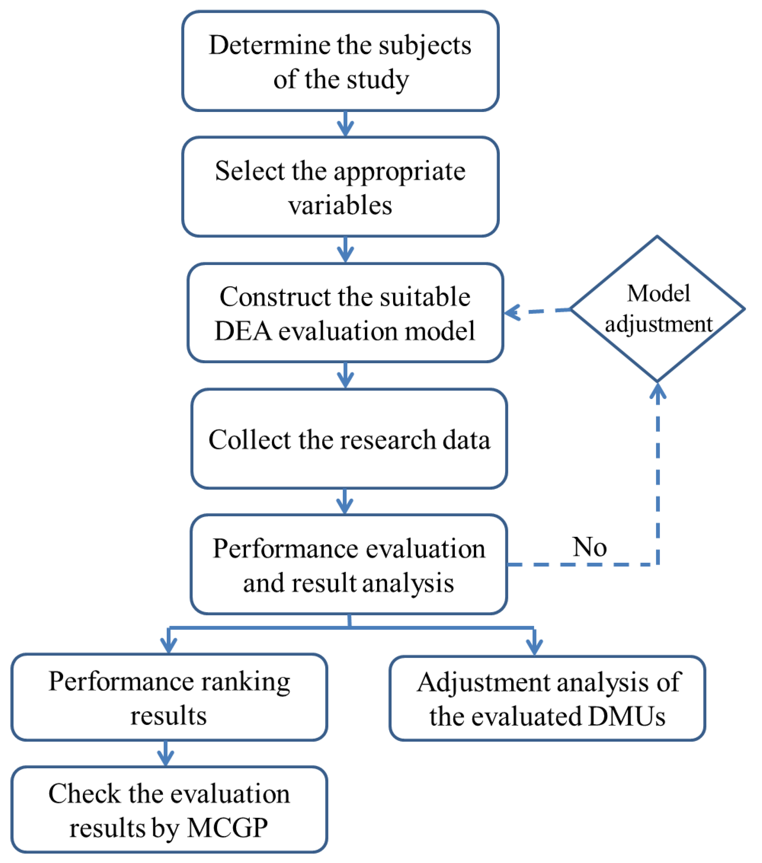
3.2. Modified SBM-DEA Model for Evaluating Green Energy Index Process

• Step 1: First, determine the research subjects of the study;
• Step 2: Select appropriate variables (green energy index) through the literature review;
• Step 3: Construct the suitable modified SBM-DEA model for the performance evaluation;
• Step 4: Based on the research results of previous steps, this study should interview some relevant enterprises to investigate the practical operational data of the selected variables;
• Step 5: Use the new proposed model (such as the new Equations (6) and (7) in this study) to conduct performance evaluation processing on the collected data. If some infeasibility problem occurs, it is necessary to go back to Step 3 and make appropriate adjustments to the constructed modified SBM-DEA model. After doing so, repeat Step 5;
• Step 6: Each evaluated DMU can obtain its super-efficiency ${{\displaystyle \varphi }}_j^{*}(j=1,\dots ,n)$ with Formulation (8);
• Step 7: Then, determine the maximum value $E_{\max }=\underset{j=1}{\overset{n}{\max }}\left\{{\varphi }_j^{*}\right\}$ to calculate the green energy index $G{I}_j(j=1,\dots ,n)$ for each evaluated DMU via Formulation (9). Based on the results of the green energy index, obtain performance ranking results and screen out the efficient benchmarking DMUs;
• Step 8: Conduct an in-depth analysis of the most suitable adjustment for the each DMU;
• Step 9: Finally, check the modified SBM-DEA model evaluation results through the MCGP method (Equations (10)–(14)).

3.3. MCGP Model for Choosing Suitable Crane Equipment

The MCGP approach encompasses the many modified GP methods in the literature. Chang (2008) developed a multi-choice aspiration level model for solving multi-objective decision-making problems [50]. A typical MCGP problem has the following structure.

In the real-world decision-making problem of choosing crane equipment, the goals are often related. This problem is represented in the following MCGP equations:

Minimize

$${\displaystyle \sum _{i=1}^n\left[({{\displaystyle d}}_i^{+}+{{\displaystyle d}}_i^{-})+({{\displaystyle e}}_i^{+}+{{\displaystyle e}}_i^{-})\right]}$$

(10)

subject to

$${{\displaystyle f}}_i(X){{\displaystyle b}}_i-{{\displaystyle d}}_i^{+}+{{\displaystyle d}}_i^{-}={{\displaystyle b}}_i{{\displaystyle y}}_{i}i=1,2,\dots ,n,$$

(11)

$${{\displaystyle y}}_i-{{\displaystyle e}}_i^{+}+{{\displaystyle e}}_i^{-}={{\displaystyle g}}_{i,\min }i=1,2,\dots ,n,$$

(12)

$${{\displaystyle g}}_{i,\min }\le {{\displaystyle y}}_i\le {{\displaystyle g}}_{i,\max }i=1,2,\dots ,,$$

(13)

$${{\displaystyle d}}_i^{+},{{\displaystyle d}}_i^{-},{{\displaystyle e}}_i^{+},{{\displaystyle e}}_i^{-}\ge 0,i=1,2,\dots ,,$$

(14)

As illustrated in Equations (11)–(13), selection restrictions are absent for any single goal, but some goals are dependent on another. For example, we can add the auxiliary constraint $b_i\le b_{i+1}+b_{i+2}$ to the MCGP model, where $b_i$, $b_{i+1}$ and $b_{i+2}$ are binary variables. Thus, $b_{i+1}$ or $b_{i+2}$ must be equal to 1 if b_i = 1. This means that if goal one was achieved, then either goal two or goal three was also achieved.

4. Empirical Research for a Real Case Example

4.1. Data Collection and Evaluating Green Performance of Various Cranes

This real-world case study aimed to evaluate the green performance of various cranes used to load and unload cargo in port operations. The four most common types of cranes used in international commercial ports, both in general and by the prominent container-handling company in Taiwan in particular, are as follows: gantry cranes (GCs), rail-mounted gantry (RMG) cranes, rubber-tired gantry (RTG) cranes, and empty container handlers (ECHs). This study collected and analyzed the 2018–2020 data on these cranes (

Table 3. Collected data and evaluation results for 2018.

DMU	Input			Output		Evaluation Results
	Working Time (Hours)	Energy Consumption (kwh)	Total Energy Cost (TWD)	Working Capacity (Moves)	CO2 Emission Volume (kg)	Efficiency	GIj *	Rank
GC	4487	534,344	1,528,224	134,595	278,928	1.07794	0.99983	2
RMG	3556	174,728	499,706	74,670	91,205	0.92779	0.86056	4
RTG	4983	235,677	674,063	109,617	123,029	1.07813	1.00000	1
ECH	4464	418,122	1,241,924	102,671	112,548	1.01733	0.94361	3

,

Table 4. Collected data and evaluation results for 2019.

DMU	Input			Output		Evaluation Results
	Working Time (Hours)	Energy Consumption (kwh)	Total Energy Cost (TWD)	Working Capacity (Moves)	CO2 Emission Volume (kg)	Efficiency	GIj *	Rank
GC	3323	445,287	1,280,598	106,811	223,893	1.09938	0.95843	2
RMG	3726	168,256	552,876	78,236	96,662	0.88134	0.76834	4
RTG	3397	117,838	485,277	74,737	84,842	1.14707	1.00000	1
ECH	3478	312,197	629,643	79,997	87,692	1.02027	0.88946	3

and

Table 5. Collected data and evaluation results for 2020.

DMU	Input			Output		Evaluation Results
	Working Time (Hours)	Energy Consumption (kwh)	Total Energy Cost (TWD)	Working Capacity (Moves)	CO2 Emission Volume (kg)	Efficiency	GIj *	Rank
GC	3712	442,106	1,388,211	63,635	123,968	1.01786	0.94071	2
RMG	3235	158,952	499,118	49,402	54,047	1.01518	0.93824	3
RTG	3313	149,582	469,690	53,008	61,514	1.08201	1.00000	1
ECH	3047	259,434	812,980	48,752	60,026	0.75103	0.69410	4

).

4.2. Modified SBM-DEA Model Analysis Result

In general, the selection of input and output variables is critical in the application of DEA. This is because the evaluation results become highly variable when the set of research variables change. The Taiwanese company investigated in this study was large and operated many cranes (including nine RMG cranes). The data for all cranes of each type also differed little. Thus, the data used in this study were the average values for each crane type.

In Table 3, Table 4 and Table 5, the basic information on each crane is presented from the second to sixth columns from the left, and the performance values, as computed using Equations (6) and (7) jointly, are presented in the seventh column from the left. The penultimate and final columns present the value of the green energy index (GI_j) and the ranking for all four crane types, respectively.

The results indicated that the green performance ranking among the cranes differed little from 2018 to 2019, and that the efficiency value of three crane types (RTG, GCs, and ECHs) exceeded 1. Thus, these three crane types operated efficiently throughout the years, with RTG cranes having the best green performance and being the most efficient. In 2020 (Table 4), in contrast to previous years, RMGs and ECHs switched rankings and the green performance of ECHs was determined to be inefficient. RTG cranes still had the best, and thus most stable, green performance and were found to be optimal for use in global commercial ports.

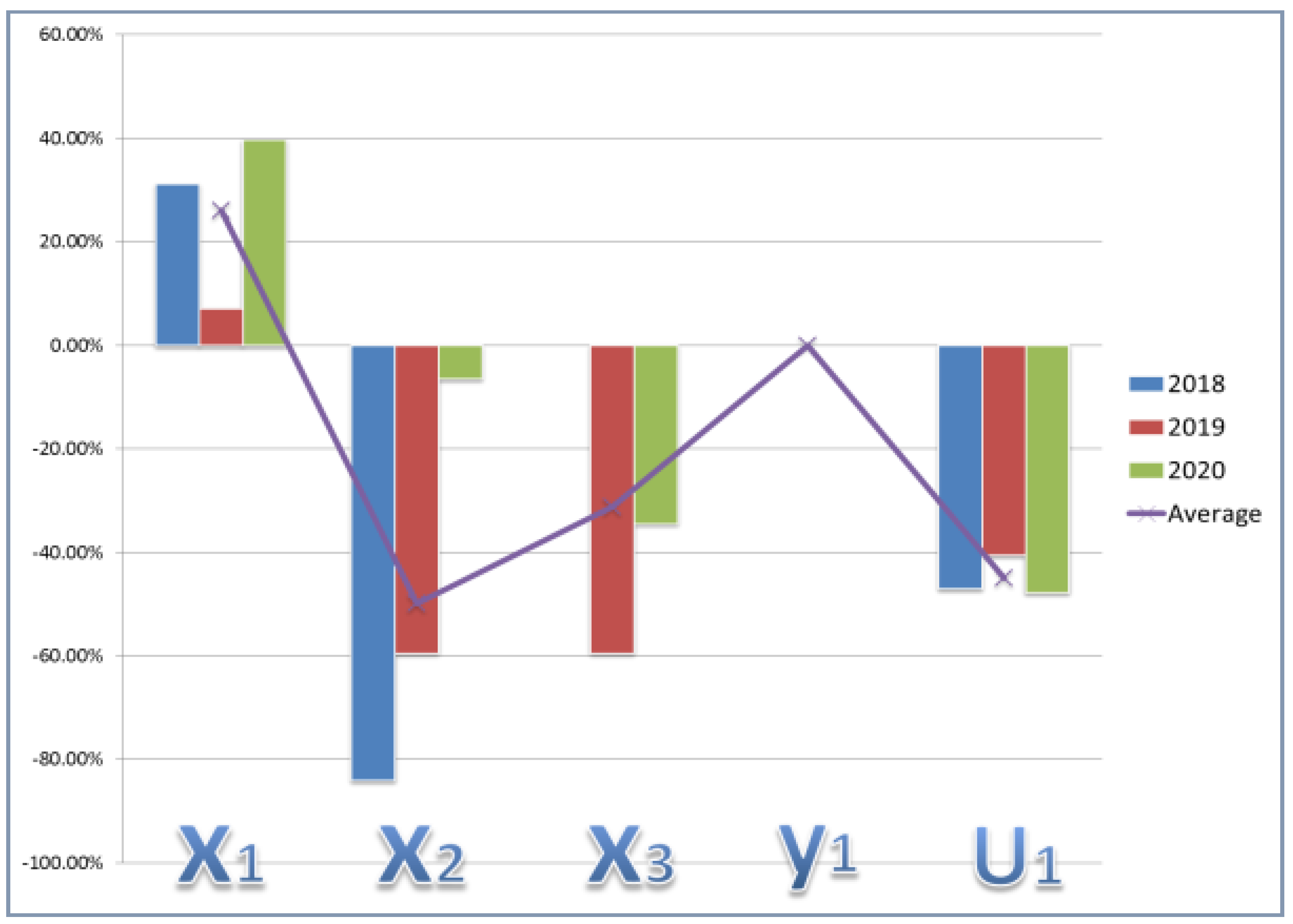
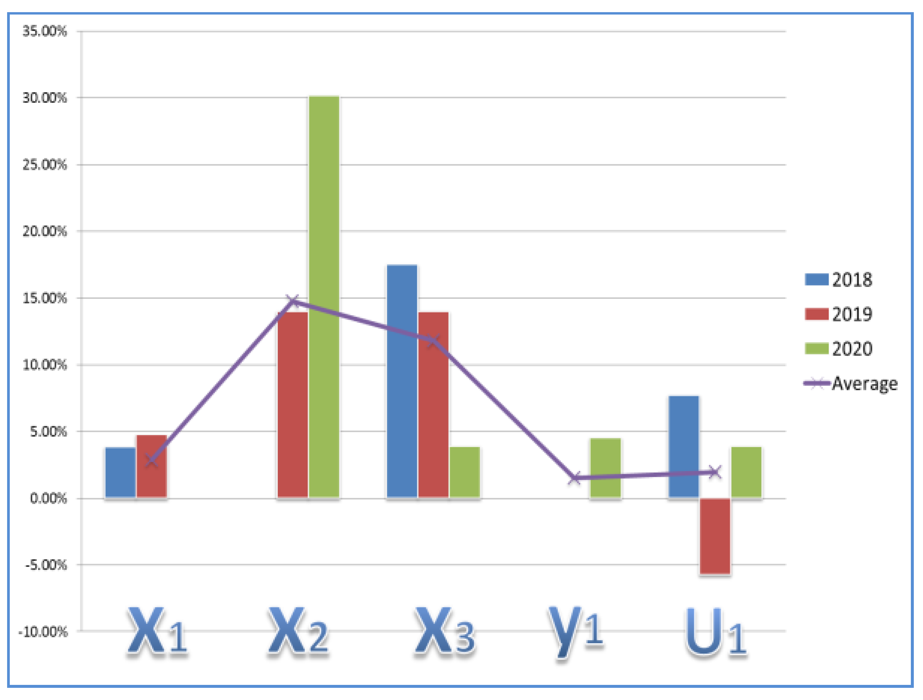
4.3. Suitable Adjustment for Each Variable Analysis

Simply providing port managers with the green performance of the four types of evaluated cranes can judge whether their operations are efficient or not, but it fails to inform them of the quantitative analysis of the advantages and disadvantages for each evaluated crane. In order to explore the advantages of efficient cranes and the disadvantages of inefficient ones, this study conducted an in-depth analysis of the most suitable adjustment for the four evaluated cranes. Then, port managers can effectively address or improve operational weaknesses, which can highlight the practical management significance and value of this study. The corresponding analysis results are presented in

Table 6. Suitable adjustment for each variable.

DMU		X1: Working Time (Hours)		X2: Energy Consumption (kWh)		X3: Total Energy Cost (TWD)		Y1: Working Capacity (Moves)		U1: CO2 Emission (kg)
		Benchmark	Change Rate *	Benchmark	Change Rate *	Benchmark	Change Rate *	Benchmark	Change Rate *	Benchmark	Change Rate *
GC	2018	5885	31.18%	85,583	−83.98%	1,528,224	0.00%	134,595	0.00%	147,983	−46.95%
	2019	3977	7.14%	179,571	−59.38%	563,853	−59.38%	63,635	0.00%	73,847	−40.43%
	2020	4644	39.75%	416,843	−6.39%	840,692	−34.35%	106,811	0.00%	117,085	−47.70%
	Ave	4835	26.02%	227,332	−49.92%	977,590	−31.24%	101,681	0.00%	112,972	−45.03%
RMG	2018	3556	0.00%	168,173	−3.75%	480,994	−3.74%	78,220	−4.75%	87,790	−3.74%
	2019	3088	−4.55%	139,407	−12.30%	437,739	−12.30%	49,402	0.00%	57,330	6.07%
	2020	3726	0.00%	129,227	−23.20%	532,175	−3.74%	81,959	−4.76%	93,042	−3.74%
	Ave	3456	−1.52%	145,602	−13.08%	483,636	−6.60%	69,861	−3.17%	79,387	−0.47%
RTG	2018	5175	3.85%	235,677	0.00%	792,201	17.53%	109,617	0.00%	132,532	7.72%
	2019	3471	4.76%	170,554	14.02%	535,548	14.02%	53,008	0.00%	57,992	−5.73%
	2020	3397	0.00%	153,429	30.20%	504,154	3.89%	71,341	4.54%	88,143	3.89%
	Ave	4014	2.87%	186,553	14.74%	610,634	11.81%	77,989	1.51%	92,889	1.96%
ECH	2018	4667	4.55%	220,741	−47.21%	631,346	−49.16%	102,671	0.00%	115,232	2.38%
	2019	3047	0.00%	137,571	−46.97%	431,974	−46.87%	48,752	0.00%	56,575	−5.75%
	2020	3636	4.55%	126,132	−59.60%	519,432	−17.50%	79,997	0.00%	90,814	3.56%
	Ave	3783	3.03%	161,482	−51.26%	527,584	−37.84%	77,140	0.00%	87,540	0.07%
Total AVE		4022	7.60%	180,242	−24.88%	649,861	−15.97%	81,667	−0.41%	93,197	−10.87%

* = positive values denote the advantage of each input and undesirable output, and negative values denote the disadvantage.

. In this table, the positive values of the change rate denote the advantage of each variable, while the negative values denote the disadvantage. For example, GCs produced an average of 278,928 kg of CO₂ emissions in 2019, but its relative benchmark value should have been 147,983 kg for that year and, as such, the decrease change rate was −46.95%. In other words, the poor performance of the GC was due to the large waste of resources in terms of carbon dioxide emissions, which is also an important reason for its relative inefficient performance. Therefore, managers should strengthen the scientific supervision at this level in future operations.

Table 6 presents the quantitative results for the tradeoff among the variables for each crane type. The results indicated the target that should be learned for each variable in a given year and the extent of adjustment (expressed in terms of an adjustment ratio) for each variable in the optimal tradeoff. For the input and undesired outputs, the adjustment ratio was calculated by subtracting the original resource value from the target value, and then dividing this difference by the original values. A positive adjustment ratio represented the performance of the learning benchmark in that direction as being not yet as good as that of the evaluated unit. In other words, a positive adjustment ratio can be interpreted as representing the advantage for a given crane type.

Conversely, if the value of the adjustment ratio for an item is negative, it represents a disadvantage for a given crane type. For good output variables, this study used reverse processing, in which the original data value was subtracted from the target value and this difference was divided by the target value. This was done to allow positive numbers to also represent advantages.

Table 6 presents the adjustment ratios for all crane types. The RTG was the best crane type with respect to all variables, especially in energy consumption and total energy cost, with average three-year advantages of 14.74% and 11.81%, respectively. The GC was the second-best crane type, and it was superior primarily in operational duration. Thus, the GC is especially advantageous when used to load and unload the same type of containers. Finally, RMG cranes and ECHs were disadvantageous due to their high energy consumption and high total energy cost. Between the two, ECHs emitted less CO₂ and had a better operational duration. These results are visualized in Figure 2, Figure 3, Figure 4 and Figure 5.

In Figure 2, Figure 3, Figure 4 and Figure 5, which each present the adjustment ratios for a given crane type for all variables, the solid line segment indicates the average value of the adjustment ratio for each year. As mentioned previously, positive and negative values indicate advantages and disadvantages, respectively. The characteristic patterns presented in these four figures remain largely consistent with those highlighted by the average evaluation results. From Figure 2, Figure 3, Figure 4 and Figure 5, the most obvious advantages and disadvantages of each evaluated DMU are clear. For example, the biggest advantages of RTG cranes are shown in the X2 and X3 levels, while the other three evaluated cranes expose the potential problem of resource waste in these two investments. Meanwhile, only RTG cranes and ECHs had certain advantages for U1 (CO₂ emission volume (kg)).

4.4. Using MCGP to Solve the Case Example of Choosing Between Crane Equipment

To solve the crane equipment selection problem of choosing between crane types, the analyst must define the MCGP model according to the following goals. In this case, suppose that the decision maker had the following set of priorities derived from the DMU results for RTG cranes in Table 5′s collected data and evaluation results for 2020 and Table 6‘s suitable adjustment for each variable RTG crane value.

To solve the problem of choosing between crane equipment problems, it is necessary to define the MCGP model according to the following goals:

• The first goal is Y1: the working capacity is the RTG benchmark. The DMU of the RTG was 71,341 and 77,989 in the Table 6 RTG 2020 results; 71,341 was the benchmark value and 77,989 was the AVE value;
• The second goal is U1: the emission volume is the RTG benchmark. The DMU of the RTG was 88,143 and 92,889 in the Table 6 RTG 2020 results;
• The third goal is X1: the operational duration is the DMU of the RTG crane’s input. The DMU of the RTG was 3397 and 4014 in the Table 6 RTG 2020 results;
• The fourth goal is X2: the energy consumption is the DMU of the RTG crane’s input. The DMU of the RTG was 153,429 and 186,553 in the Table 6 RTG 2020 results;
• The fifth goal is X3: the total energy cost is the DMU of the RTG crane’s input. The DMU of RTG was 504,154 and 610,634 in the Table 6 RTG 2020 results.

Table 7. Coefficient and goal values for MCGP model.

					Choice
	S1	S2	S3	S4	Choice Value	Goal
U1	123,968	54,047	61,514	60,026	(71,341, 77,989)	CO2 Emission volume benchmark value
Y1	63,635	49,402	53,008	48,752	(88,143, 92,889)	Working capacity benchmark value
X1	−3712	3235	3313	3047	(3397, 4014)	Energy consumption benchmark value
X2	442,106	158,952	149,582	259,434	(153,429, 186,553)	Energy consumption benchmark value
X3	1,388,211	499,118	469,690	812,980	(504,154, 610,634)	Total Energy cost benchmark value

provides the coefficient and goal values for solving the MCGP crane equipment selection problem.

The MCGP model notation is introduced as follows:

• Indices:

i 1,2,…, n index of crane equipment type;

j 1,2,…, j index of deviation corresponding to the goals.

• Parameters:

U1_j is the CO₂ emission volume of crane equipment type j, where j =1, 2, 3, 4;

Y1_j is the working capacity of crane equipment type j, where j =1, 2, 3, 4;

X1_j is the energy consumption of crane equipment type j, where j =1, 2, 3, 4;

X2_j is the energy consumption of crane equipment type j, where j =1, 2, 3, 4;

X3_j is the total energy cost of crane equipment type j, where j =1, 2, 3, 4;

$d_j^{+}$, $d_j^{-}$ are the maximum and minimum deviation of goal j;

$e_t^{+}$, $e_t^{-}$ are the maximum and minimum deviation of $\left|y_t-g_{i,\max /\min }\right|$.

• Decision variables:

X_i is the order quantity of vendor i;

y_i is the binary integer $\{\begin{array}{cc}1& if\begin{array}{l}\hfill \end{array}the\begin{array}{l}\hfill \end{array}order\begin{array}{l}\hfill \end{array}is\begin{array}{c}\end{array}offered\begin{array}{c}\end{array}by\begin{array}{c}\end{array}crane\begin{array}{c}euipment\end{array}i\\ 0& otherwise\end{array}$

We provide the following MCGP model programming in

Table 8. MCGP model solution programming for the crane equipment section.

MCGP Model Solution Programming	MCGP Model Goal
Min z=	Objection function
dp1 + dn1 + ep1 + en1)	Satisfy the first goal
+(dp2 + dn2 + ep2 + en2)	Satisfy the second goal
+(dp3 + dn3 + ep3 + en3)	Satisfy the third goal
+dp4 + dn4 + ep4 + en4)	Satisfy the fourth goal
+(dp5 + dn5 + ep5 + en5)	Satisfy the fifth goal
s.t	(63,635s1 + 49,402s2 + 53,008s3 + 48,752s4) + dn1 − dp1 = y1b1 For the first goal, the less the better
y1 − ep1 + en1 = 71,341	For $\left|y_1-g_{1,\min }\right|$
y1 71,341 y1 ≤ 77,989	For bound of the y1
12,3968s1 + 54,047s2 + 61,514s3 + 60,026s4 + dn2 − dp2 = y2b2 For the second goal, the less the better y2 − ep2 + en2 = 88,143	For $\left|y_2-g_{2,\min }\right|$
y2 $\ge$ 88,143 y2 92,889	For bound of the y2
3712s1 + 3235s2 + 3313s3 + 3047s4 = y3b3	For the third goal, the less the better
y3 − ep3 + en3 = 3397	For $\left|y_3-g_{3,\min }\right|$
y3 $\ge$ 3397 y3 4014	For bound of the y3
44,2106s1 + 158,952s2 + 149,582s3 + 259,434s4 = y4b4	For the fourth goal, the less the better
y4 − ep4 + en4 = 153,429	For $\left|y_4-g_{4,\min }\right|$
y4 $\ge$ 153429 y4 186553	For bound of the y4
1,388,211s1 + 499,118s2 + 469,690s3 + 12,980s4 = y5b5	For the fifth goal, the less the better
y5 − ep5 + en5 = 504,154	For $\left|y_5-g_{5,\min }\right|$
y5 $\ge$ 504,154 y5 610,634	For bound of the y5
s1 + s2 +s3 + s4 = 1	To selection crane equipment
b1 = b2 + b3 + b4	For ensuring the goals, and zero should be achieved
b2 + b3 + b4 = 1	Added auxiliary constraints can force the goals (such that the lower-bound goal is achieved)
si >= 0, i = 1, 2, 3,4, $d_i^{+}$, $d_i^{-}$, $e_i^{+}$, $e_i^{-}$ $\ge 0$, i = 1, 2, … 5.

:

min ${{\displaystyle d}}_1^{+}+{{\displaystyle d}}_1^{-}+{{\displaystyle d}}_2^{+}+{{\displaystyle d}}_2^{-}+{{\displaystyle d}}_3^{+}+{{\displaystyle d}}_3^{-}+{{\displaystyle d}}_4^{-}+{{\displaystyle d}}_5^{-}+{{\displaystyle e}}_1^{+}+{{\displaystyle e}}_1^{-}+{{\displaystyle e}}_2^{+}+{{\displaystyle e}}_2^{-}+{{\displaystyle e}}_3^{+}+{{\displaystyle e}}_3^{-}+{{\displaystyle e}}_4^{+}+{{\displaystyle e}}_4^{-}+{{\displaystyle e}}_5^{+}+{{\displaystyle e}}_5^{-}$y1 − ${{\displaystyle e}}_1^{+}$ + ${{\displaystyle e}}_1^{-}$ = 71,341; y1 ≥ 71,341; y1 ≤ 77,989

123,968s1 + 54,047s2 + 61,514s3 + 60,026s4 + ${{\displaystyle d}}_1^{-}$ − ${{\displaystyle d}}_1^{+}$ = y2b2

y2 − ${{\displaystyle e}}_2^{+}$ + ${{\displaystyle e}}_2^{-}$ = 88,143; y2$\ge$88,143; y2 <= 92,889

3712s1 + 3235s2 + 3313 s3 + 3047s4 $\le$ y3b3

y3 − ${{\displaystyle e}}_3^{+}$ + ${{\displaystyle e}}_3^{-}$ = 3397; y3 ≥ 3397; y3 $\le$ 4014;

442,106s1 + 158,952s2 + 149,582s3 + 259,434s4 = y4b4

y4 − ${{\displaystyle e}}_4^{+}$ + ${{\displaystyle e}}_4^{-}$ = 153,429; y4 $\ge$ 153,429; y4 $\le$ 186,553;

1,388,211s1 + 499,118s2 + 469,690 s3 + 12,980s4 = y5b5;

y5 − ${{\displaystyle e}}_5^{+}$ + ${{\displaystyle e}}_5^{-}$ = 504,154; y5 ≥ 5 $\ge$ 04,154; y5 $\le$ 610,634;

s1 + s2 + s3 + s4 = 1;

b1 = b2 + b3 + b4;

b2 + b3 + b4 = 1;

s_i >= 0, i = 1, 2, 3, 4

${{\displaystyle d}}_i^{+}$, ${{\displaystyle d}}_i^{-}$, ${{\displaystyle e}}_i^{+}$, ${{\displaystyle e}}_i^{-}$ $\ge 0$, i = 1, 2, … 5.

Using Lingo software [51], we obtained the following solution: s1 = 0, s2 = 0, s3 = 1, and s4 = 0; y1 = 71,341, y2 = 88,143, y3 = 4014, y4 = 186,553, and y5 = 504,154. This means that the RTG crane is a suitable crane [52].

5. Conclusions and Implications

5.1. Conclusions

Green ports are becoming increasingly prominent with the increased need for environmental protection globally. However, few studies have monitored exhaust or PM emissions (such as CO₂ or sulfide) around ports due to the difficulty of doing so, and the data obtained are incomplete.

To fill this gap in the literature, this study measured CO₂ emissions at their source, specifically container-handling cranes (which are indispensable to port operations). Five key variables, including CO₂ emissions, were identified based on consultations with experts. Subsequently, (1) we applied a method that combined a modified SBM-DEA model with the MCGP method to account for undesirable outputs, and (2) we defined a novel green energy index to evaluate green performance. Our findings determined (1) the crane type with the best green performance, and (2) how advantages and disadvantages are balanced in the use of each crane type. These findings can help port managers select the best crane equipment that makes their port greener, smarter, and more profitable.

5.2. Managerial Implications

We present the following managerial prescriptions based on our findings. First, we recommend RTG cranes because they are the most environmentally friendly when used in international commercial ports and strike the best tradeoff between environmental protection and profitability. Second, RMG cranes and ECHs consume considerable energy, which constitutes a point of concern that port managers must pay attention to. Third, to mitigate environmental harm and commercial loss, port managers should replace outdated equipment or, if they are unable to do so, supervise outdated equipment more intensely. Fourth, port managers can invest more in researching and developing smarter port equipment, which incorporates, for example, big data or Internet of Things technology. Smart port equipment minimizes operational waste and, thus, mitigates their environmental impact and enhances profitability.

5.3. Limitations

(i)

To mitigate the disadvantages of the DEA method, we used the MCGP method to verify the DEA results. To better cope with uncertainty, decision makers can use the novel MCGP method in conjunction with the multi-criteria decision-making approach;

(ii)

Our study, a real-world case example, used data collected in Taiwan.

5.4. Future Directions

Future studies can use other new DEA methods to solve crane equipment selection problems. Additionally, other mathematical models, such as new MCGP models, can be combined with our study’s model.

References

1. Carey, M. In The Shadow of Melting Glaciers: Climate Change and Andean Society; Oxford University Press: New York, NY, USA, 2010. [Google Scholar]
2. Barragán, J.M.; de Andrés, M. Analysis and trends of the world’s coastal cities and agglomerations. Ocean Coast. Manag. 2015, 114, 11–20. [Google Scholar] [CrossRef]
3. Chang, C.-C.; Wang, C.-M. Evaluating the effects of green port policy: Case study of Kaohsiung harbor in Taiwan. Transp. Res. Part D Transp. Environ. 2012, 17, 185–189. [Google Scholar] [CrossRef]
4. Wan, C.; Zhang, D.; Yan, X.; Yang, Z. A novel model for the quantitative evaluation of green port development—A case study of major ports in China. Transp. Res. Part D Transp. Environ. 2018, 61, 431–443. [Google Scholar] [CrossRef]
5. Barnes-Dabban, H.; Van Tatenhove, J.P.M.; Van Koppen, K.C.S.A.; Termeer, K.J.A.M. Institutionalizing environmental re-form with sense-making: West and central Africa ports and the ‘green port’ phenomenon. Mar. Policy 2017, 86, 111–120. [Google Scholar] [CrossRef]
6. Meng, B.; Kuang, H.; Niu, E.; Li, J.; Li, Z. Research on the Transformation Path of the Green Intelligent Port: Outlining the Perspective of the Evolutionary Game “Government–Port–Third-Party Organization”. Sustainability 2020, 12, 8072. [Google Scholar] [CrossRef]
7. Twrdy, E.; Zanne, M. Improvement of the sustainability of ports logistics by the development of innovative green infra-structure solutions. Transp. Res. Procedia 2020, 45, 539–546. [Google Scholar] [CrossRef]
8. Liu, P.; Wang, C.; Xie, J.; Mu, D.; Lim, M.K. Towards green port-hinterland transportation: Coordinating railway and roadin-frastructure in Shandong Province, China. Transp. Res. D Transp. Environ. 2021, 94, 102806. [Google Scholar] [CrossRef]
9. Espino, G.D.L.L.; Rodríguez, I.P.; Czitrom, S.P. Water quality of a port in NW Mexico and its rehabilitation with swell energy. Mar. Pollut. Bull. 2010, 60, 123–130. [Google Scholar] [CrossRef]
10. Otene, B.B.; Nnadi, P. Water Quality Index and Status of Minichinda Stream, Port Harcourt, Nigeria. IIARD Int. J. Geogr. Environ. Manag. 2019, 5, 1–9. [Google Scholar]
11. Lee, S.; Lee, E.; Yoo, H.S.; Lee, M.J. Analysis of trends in marine water quality using environmental impact as-sessment monitoring data: A case study of Busan new port. J. Coast. Res. 2020, 102, 39–46. [Google Scholar] [CrossRef]
12. Bolognese, M.; Fidecaro, F.; Palazzuoli, D.; Licitra, G. Port Noise and Complaints in the North Tyrrhenian Sea and Frame Work for Remediation. Environments 2020, 7, 17. [Google Scholar] [CrossRef] [Green Version]
13. Di Vaio, A.; Varriale, L.; Trujillo, L. Management Control Systems in port waste management: Evidence from Italy. Util. Policy 2019, 56, 127–135. [Google Scholar] [CrossRef]
14. Prati, M.V.; Costagliola, M.A.; Quaranta, F.; Murena, F. Assessment of ambient air quality in the port of Naples. J. Air Waste Manag. Assoc. 2015, 65, 970–979. [Google Scholar] [CrossRef] [PubMed] [Green Version]
15. Kontos, S.; Liora, N.; Poupkou, A.; Giannaros, C.; Garane, K.; Melas, D. Air-Quality Impact of Cruise and Passenger Ship Emissions in the Port of Thessaloniki. Springer Atmos. Sci. 2017, 1129–1134. [Google Scholar] [CrossRef]
16. Casazza, M.; Lega, M.; Jannelli, E.; Minutillo, M.; Jaffe, D.; Severino, V.; Ulgiati, S. 3D monitoring and modelling of air quality for sustainable urban port planning: Review and perspectives. J. Clean. Prod. 2019, 231, 1342–1352. [Google Scholar] [CrossRef]
17. Progiou, A.G.; Bakeas, E.; Evangelidou, E.; Kontogiorgi, C.; Lagkadinou, D.; Sebos, I. Air pollutant emissions from Pi-raeusport: External costs and air quality levels. Transp. Res. D Transp. Environ. 2021, 91, 102586. [Google Scholar] [CrossRef]
18. Gobbi, G.P.; Di Liberto, L.; Barnaba, F. Impact of port emissions on EU-regulated and non-regulated air quality indicators: The case of Civitavecchia (Italy). Sci. Total. Environ. 2020, 719, 134984. [Google Scholar] [CrossRef]
19. Ee, J.Y.C.; Chan, J.Y.; Kang, G.L. Carbon reduction analysis of Malaysian green port operation. Prog. Energy Environ. 2021, 15, 1–7. [Google Scholar]
20. Fabregat, A.; Vázquez, L.; Vernet, A. Using Machine Learning to estimate the impact of ports and cruise ship traffic on urbanair quality: The case of Barcelona. Environ. Model. Softw. 2021, 139, 104995. [Google Scholar] [CrossRef]
21. Li, J.; Hu, Z.; Shi, V.; Wang, Q. The benefit of manufacturer encroachment considering consumer’s environmental awarenessand product competition. Ann. Oper. Res. 2021, in press. [Google Scholar]
22. Li, J.; Hu, Z.; Shi, V.; Wang, Q. Manufacturer’s encroachment strategy with substitutable green products. Int. J. Prod. Econ. 2021, 235, 108102. [Google Scholar] [CrossRef]
23. Budiyanto, M.A.; Huzaifi, M.H.; Sirait, S.J.; Prayoga, P.H.N. Evaluation of CO2 emissions and energy use with different container terminal layouts. Sci. Rep. 2021, 11, 1–14. [Google Scholar] [CrossRef]
24. Dong, G.; Zhu, J.; Li, J.; Wang, H.; Gajpal, Y. Evaluating the Environmental Performance and Operational Efficiency of Container Ports: An Application to the Maritime Silk Road. Int. J. Environ. Res. Public Health 2019, 16, 2226. [Google Scholar] [CrossRef] [PubMed] [Green Version]
25. Abu Aisha, T.; Ouhimmou, M.; Paquet, M. Optimization of Container Terminal Layouts in the Seaport—Case of Port of Montreal. Sustainability 2020, 12, 1165. [Google Scholar] [CrossRef] [Green Version]
26. Li, J.; Wang, F.; He, Y. Electric Vehicle Routing Problem with Battery Swapping Considering Energy Consumption and Carbon Emissions. Sustainability 2020, 12, 10537. [Google Scholar] [CrossRef]
27. Charnes, A.; Cooper, W.W.; Rhodes, E. Measuring the efficiency of decision making units. Eur. J. Oper. Res. 1978, 2, 429–444. [Google Scholar] [CrossRef]
28. Banker, R.D.; Charnes, A.; Cooper, W.W. Some models for estimating technical and scale inefficiencies in data envel-opment analysis. Manag. Sci. 1984, 30, 1078–1092. [Google Scholar] [CrossRef] [Green Version]
29. Andersen, P.; Petersen, N.C. A Procedure for Ranking Efficient Units in Data Envelopment Analysis. Manag. Sci. 1993, 39, 1261–1264. [Google Scholar] [CrossRef]
30. Zhu, J. Super-efficiency and DEA sensitivity analysis. Eur. J. Oper. Res. 2001, 129, 443–455. [Google Scholar] [CrossRef]
31. Lee, H.S.; Chou, M.T.; Kuo, S.G. Evaluating port efficiency in Asia Pacific region with recursive data envelopment analysis. J. East. Asia Soc. Transp. Stud. 2005, 6, 544–559. [Google Scholar]
32. Tovar, B.; Wall, A. Environmental efficiency for a cross-section of Spanish port authorities. Transp. Res. Part D Transp. Environ. 2019, 75, 170–178. [Google Scholar] [CrossRef]
33. Wang, L.; Zhou, Z.; Yang, Y.; Wu, J. Green efficiency evaluation and improvement of Chinese ports: A cross-efficiency model. Transp. Res. Part D Transp. Environ. 2020, 88, 102590. [Google Scholar] [CrossRef]
34. Tone, K. A slacks-based measure of efficiency in data envelopment analysis. Eur. J. Oper. Res. 2001, 130, 498–509. [Google Scholar] [CrossRef] [Green Version]
35. Na, J.-H.; Choi, A.-Y.; Ji, J.; Zhang, D. Environmental efficiency analysis of Chinese container ports with CO2 emissions: An inseparable input-output SBM model. J. Transp. Geogr. 2017, 65, 13–24. [Google Scholar] [CrossRef]
36. Wang, C.-N.; Day, J.-D.; Lien, N.T.K.; Chien, L.Q. Integrating the Additive Seasonal Model and Super-SBM Model to Compute the Efficiency of Port Logistics Companies in Vietnam. Sustainability 2018, 10, 2782. [Google Scholar] [CrossRef] [Green Version]
37. Xiao, Y.; Qi, G.; Jin, M.; Yuen, K.F.; Chen, Z.; Li, K.X. Efficiency of Port State Control Inspection Regimes: A Compara-tive Study. Transp. Policy 2021, 106, 165–172. [Google Scholar] [CrossRef]
38. Wanke, P.F. Physical infrastructure and shipment consolidation efficiency drivers in Brazilian ports: A two-stage net-work-DEA approach. Transp. Policy 2013, 29, 145–153. [Google Scholar] [CrossRef]
39. Chao, S.-L.; Yu, M.-M.; Hsieh, W.-F. Evaluating the efficiency of major container shipping companies: A framework of dynamic network DEA with shared inputs. Transp. Res. Part A Policy Pr. 2018, 117, 44–57. [Google Scholar] [CrossRef]
40. Saeedi, H.; Behdani, B.; Wiegmans, B.; Zuidwijk, R. Assessing the technical efficiency of intermodal freight transport chains using a modified network DEA approach. Transp. Res. Part E Logist. Transp. Rev. 2019, 126, 66–86. [Google Scholar] [CrossRef]
41. Kwon, D.S.; Cho, J.H.; Sohn, S.Y. Comparison of technology efficiency for CO2 emissions reduction among European coun-tries based on DEA with decomposed factors. J. Clean. Prod. 2017, 151, 109–120. [Google Scholar] [CrossRef]
42. Cui, Q. Investigating the airlines emission reduction through carbon trading under CNG2020 strategy via a Network Weak Disposability DEA. Energy 2019, 180, 763–771. [Google Scholar] [CrossRef]
43. Yang, M.; Hou, Y.; Ji, Q.; Zhang, D. Assessment and optimization of provincial CO2 emission reduction scheme in China: An improved ZSG-DEA approach. Energy Econ. 2020, 91, 104931. [Google Scholar] [CrossRef]
44. Ren, F.R.; Tian, Z.; Liu, J.; Shen, Y.T. Analysis of CO2 emission reduction contribution and efficiency of China’s solar photo-voltaic industry: Based on input-output perspective. Energy 2020, 199, 117493. [Google Scholar] [CrossRef]
45. Li, Y.; Li, J.; Gong, Y.; Wei, F.; Huang, Q. CO2 emission performance evaluation of Chinese port enterprises: A modified me-ta-frontier non-radial directional distance function approach. Transp. Res. D Transp. Environ. 2020, 89, 102605. [Google Scholar] [CrossRef]
46. Wang, Z.; Wu, X.; Guo, J.; Wei, G.; Dooling, T.A. Efficiency evaluation and PM emission reallocation of China ports based on improved DEA models. Transp. Res. Part D Transp. Environ. 2020, 82, 102317. [Google Scholar] [CrossRef]
47. Charnes, A.; Cooper, W.W. Programming with linear fractional functionals. Nav. Res. Logist. Q. 1963, 10, 273–274. [Google Scholar] [CrossRef]
48. Tone, K. A slacks-based measure of super-efficiency in data envelopment analysis. Eur. J. Oper. Res. 2002, 143, 32–41. [Google Scholar] [CrossRef] [Green Version]
49. Fang, H.-H.; Lee, H.-S.; Hwang, S.-N.; Chung, C.-C. A slacks-based measure of super-efficiency in data envelopment analysis: An alternative approach. Omega 2013, 41, 731–734. [Google Scholar] [CrossRef]
50. Chang, C.-T. Revised multi-choice goal programming. Appl. Math. Model. 2008, 32, 2587–2595. [Google Scholar] [CrossRef]
51. Schrage, L. LINGO Release 8.0; LINGO System Inc.: Chicago, IL, USA, 2002. [Google Scholar]
52. Shen, C.-W.; Peng, Y.-T.; Tu, C.-S. Multi-Criteria Decision-Making Techniques for Solving the Airport Ground Handling Service Equipment Vendor Selection Problem. Sustainability 2019, 11, 3466. [Google Scholar] [CrossRef] [Green Version]
Figure 1. Flow chart for the DEA application.
Sustainability 13 06801 g001
Figure 2. Adjustment ratios for GCs.
Sustainability 13 06801 g002
Figure 3. Adjustment ratios for RMG cranes.
Sustainability 13 06801 g003
Figure 4. Adjustment ratios for RTG cranes.
Sustainability 13 06801 g004
Figure 5. Adjustment ratios for ECHs.
Sustainability 13 06801 g005