Territorial-Based vs. Consumption-Based Carbon Footprint of an Urban District—A Case Study of Berlin-Wedding

Abstract

Cities account for 70% of carbon emissions and are therefore a vital driver for climate change. Thus, a city’s main contributing sectors need to be identified. Territorial-based footprints focus on the final energy consumption, which is derived from the stationary and transport sectors. The consumption-based approach is based on consumption data, which are converted into carbon emissions using an input–output model. If the consumption-based approach is applied to an urban district not only emissions in the investigated area are considered, but also those that occur along the supply chain of consumed products in the urban district. The goal of this study was to apply and evaluate two different approaches to calculate an urban district’s carbon footprint to support climate protection management at the local government level. To achieve this goal, these two different approaches were applied to calculate the carbon emissions of the urban district Wedding in Berlin and were compared regarding criteria such as data availability and relevance. The footprints resulted in 400,947 t CO₂-eq. for the territorial approach and in 401,371 t CO₂-eq. per year for the consumption-based approach, which resulted in 4.61 t CO₂-eq and 4.62 t CO₂-eq per capita and year, respectively. Methodologically, the two approaches differ significantly, but the total results showed a difference of only 0.1%. Thus, this study cannot verify that the consumption-based approach mostly leads to higher emissions per capita in the Global North. This could be due to lower purchasing power and a higher share of multiple-person households in the relatively poor urban district of Wedding, Berlin. The territorial approach is more suitable to derive measures for local climate action, whereas the consumption-based approach highlights the responsibility of consumers for GHG emissions along the supply chain and the importance of the food sector.

1. Introduction

Today, more than half of the global population live in cities. Following a constant increase by the year 2050, even two-third of global citizens will be living in cities. According to the United Nations Development Programme (UNDP), cities “occupy just 3% of the Earth’s land but account for 60 to 80% of energy consumption and at least 70% of carbon emissions” [1]. Looking at cities through the lens of climate change, cities are a crucial factor [1]. To tackle the challenge of climate change, carbon emissions need to be reduced drastically, especially in cities [2,3]. In order to formulate carbon reduction targets, emissions must be calculated first. Different studies propose methods and tools for the carbon accounting of cities [4,5]. The calculation models differ in their approach and methodology of accounting. In the following, the most applied and discussed approaches are introduced. Territorial-based carbon accounting is the approach traced back to the Kyoto Protocol. The beginning of territorial-based accounting is based on the guidelines by the Intergovernmental Panel on Climate Change for the accounting of national greenhouse gas (GHG) emissions [6]. The guidelines explain the approach of carbon accounting as “national inventories include greenhouse gas emissions and removals taking place within national territory and offshore areas over which the country has jurisdiction” [6]. Traditionally, carbon emissions of regions are calculated using the territorial-based approach. Different carbon emissions scopes were defined for emission accounting and associated carbon footprints of organizations [7,8,9]. In 2014, these scope definitions were also extended to cities in a guideline by the World Resource Institute (WRI) proposing a calculation standard for the carbon accounting of cites [5].

The WRI defines the scopes for cities as follows [5]:

• Scope 1: GHG emissions from sources located within the city boundary;
• Scope 2: GHG emissions occurring as a consequence of the use of grid-supplied electricity, heat, steam and/or cooling within the city boundary;
• Scope 3: All other GHG emissions that occur outside the city boundary as a result of activities taking place within the city boundary.

There is no consistent interpretation of these scopes in terms of urban carbon footprint yet. Most studies, e.g., Chen et al. [10], consider at least scope 1 emissions as territorial-based and scope 1 + 2 + 3 emissions as consumption-based [11,12,13]. However, for some years now, the question has been discussed in the scientific community whether the territorial-based approach, that mostly only covers scope 1 and, optionally, scope 2 emissions, may lead to injustices between the Global South, where a large part of products are produced, and the Global North, where these products are consumed [14,15,16,17]. Critique of the territorial approach for national accounting was formulated amongst others by Peter and Hertwich [18] who proposed a consumption-based accounting system. The critique is often connected to the term “carbon leakage.” This term describes the situation where companies move their production facilities to countries with lower climate regulations because of higher costs concerning climate regulations in their original production country [15,17,19]. The territorial-based approach might be fostering this practice, as it enables a shift of responsibility for carbon emissions from countries in the Global North to countries in the Global South [20]. There are already studies comparing the two approaches at the national level [16,21] and also at the city level [12,22], but, to date, there is no study that compared them at the urban district level. The district level is important, as cities often have a high level of greenhouse gas differentiation and necessary action might differ based on different urban forms and different income levels of the population within a city. We suspect that there will not be a one-size-fits-all solution for city center areas and suburbs, and the local governments of big cities such as Berlin can develop district-specific measures. With a city-level focus, such differentiation will be blurred and rendered visible with a smaller scale such as the urban district. Liu et al. [23] proposed that more micro-level research should be carried out on the city- or household-level, and the district level in this study lies in between those and can therefore enable valuable insights. We chose the Wedding district in Berlin, as previously studies on Charlottenburg-Wilmersdorf (a relatively wealthy area in Berlin) have been performed, and we also wanted to evaluate the socio-economic effect of evaluating a relatively poorer urban district with a high unemployment rate. Bakó et al. [24] studied the household energy consumption of different cities and found that unemployment is a key factor that decreases CO₂ emissions from energy consumption; we also wanted to test this assumption.

The goal of this study was to compare the territorial- and consumption-based approaches of carbon accounting or greenhouse gas accounting of cities for an urban district to identify strengths and weaknesses of these approaches and to determine which approach fits best to derive climate action at a district level. It therefore aimed to provide climate protection managers and the local government guidance regarding which approach best suits their purpose, and therefore it assessed the approaches regarding their applicability, the availability of data, and the reproducibility and relevance of the results. In order to reach this goal, these two different approaches were applied in a case study to calculate the carbon emissions of the northern Berlin urban district Wedding in the northwest of Berlin, Germany. There are 86,929 people living in Wedding [25]. The city administration states on their website for Wedding that it belongs to the “socially weaker districts” [26].

Following this introduction, Section 2 provides an insight into the methods and data used to conduct the case study and the comparison of the territorial- and consumption-based approach. The presentation of the results is provided in Section 3 and the results are discussed in Section 4, followed by a brief conclusion.

2. Materials and Methods

In this section, the materials and methods are outlined beginning with the applied territorial- and consumption-based accounting approaches and followed by the goal and scope of the case study. The territorial- and consumption-based approaches were applied separately to allow a comprehensive comparison later on. In the following, the two approaches and the respective calculations are explained, and the conduction of the case study is illustrated. The steps to carry out the case studies and compare the approaches are visualized in Figure 1.

2.1. Territorial-Based Carbon Accounting

Territorial-based emissions are those that occur within the boundary of a territory and therefore consider scope 1. Most studies though also consider scope 2 and even some consider scope 3 emissions to be territorial emissions [7,8]. A variety of definitions are available that have different scopes [8,11,22,27,28,29,30]. In Germany, the Institut für Energie- und Umweltforschung published a territorial-based standard called BISKO that aims to harmonize different approaches and achieve comparability between carbon accounting of German municipalities [28]. Many municipalities in Germany have used the BISKO standard so far, and therefore, we applied it in this study. The calculations of the territorial-based carbon footprint build on the publication from Hertle et al. [28], which describes the method that is used by the BISKO standard. The BISKO standard is defined as a final energy-based territorial carbon accounting. Within a territory, all accruing consumption on the level of final energy is considered and assigned to various sectors, for example, housing or traffic. The carbon emissions are calculated through specific emission factors [31,32,33]. Thus, emissions of scope 1 and scope 2 are considered. With the use of emission factors, CO₂ equivalents and upstream emissions for the stationary and the transport sectors are included into the accounting [28]. The standard does not predefine but proposes consumption sectors and emission factors. Table S1 in the Supplementary Materials displays the emission factors used in this study. Energy consumption of the stationary sector (electricity, natural gas, district heat) were based on the Energy Atlas Berlin [34]. Heating oil, coal, lignite, biomass, and solar thermal energy were neglected because of a statement of the district chimney sweeper, who takes care of those heating systems. As there are almost no single-family houses but apartment buildings, the neglected energy types play a minor role in the heat supply of the district. For the traffic sector, traffic activity data and timetables were used [35,36,37]. The BISKO standard may not be suitable for other countries, because of different energy consumption patterns that are not determined by centralized systems and thus inconsistent emission factors [38]; however, for the German situation, it fits well.

2.2. Consumption-Based Carbon Accounting

The critique of the territorial-based accounting approach led to the development of consumption-based accounting. The principle of consumption-based carbon accounting assigns the responsibility of emissions to the consumers of products and services rather than to the producers [39]. For consumption-based carbon accounting, the definitions are not as various, but the methods applied are even more diverse. Consumption-based carbon footprints calculate emissions that are related to consumption activities within a city. A simplified calculation for consumption-based carbon accounting is displayed in Equation (1) derived from Chen et al. [7].

GHG_consumption = GHG_territorial + GHG_imports − GHG_exports

(1)

To calculate carbon emissions that correspond to the consumption, information on the consumption of people must be available. Although there is no specific consumption information available for the urban district of Wedding, a consumer expenditure survey (CES) for Berlin exists [40]. The expenditure data lists expenses of households in Berlin for food, drinks, tobacco, clothing, living, household furniture, health care, traffic, and entertainment. In order to evaluate consumption activities in Wedding, the expenditure data must be scaled to the population in Wedding. The only specific data available concerning the structure of the population in Wedding was the age distribution of its citizens, the proportion of foreigners, and the share of people that receive a basic income. In the expenditure survey, the consumption data is given per household and not per person. In order to obtain the total expenditure of Wedding, the distribution of households was assumed to be the same as for the whole of Mitte, Berlin (Table S2 in the Supplementary Materials) as no Wedding-specific data was available. Based on these percentages, it was possible to calculate the percentage of people in Wedding living in predefined household sizes and how many households exist in Wedding; this was then multiplied with the expenditure data and scaled up to one year, resulting in the yearly consumption of all citizens in Wedding.

For the consumption-based accounting, the Exiobase data set with input–output matrices was used [41]. The CES data is given in purchaser price, whereas the Exiobase data is in base price, so the CES data was converted into base price. For the conversion of each consumption category in the CES data taxes, margins and subsidies were researched resulting in specific base price/purchaser price ratios (Table S3 in the Supplementary Materials). The consumption categories in the CES data differed from the sectors in the Exiobase data. One consumption category can correspond to one or multiple sectors from the Exiobase data set and vice versa. To transfer the CES data into the Exiobase sectors, the method from Pichler et al. [42] was used. A correspondence matrix C_nxm was set up where n represents the consumption categories of CES data and m the sectors in the Exiobase data. If a consumption category corresponded to a sector, the entry was 1; otherwise, it was 0. Analogously to Pichler et al. [42], the assumption was made that the corresponding ratio between sectors and consumption categories was the same on national and urban levels. Therefore, the correspondence matrix was multiplied per column with the domestic final demand and then normalized first per row (each entry was divided by its row sum) and per column (each entry was divided by its column sum). These calculations resulted in the coefficient correspondence matrix C′. The final demand vector for Wedding (Y′) can be calculated as

$$Y^{\prime }=C^{\prime }\ast x$$

(2)

where x is the CES vector of Wedding.

The final demand vector Y′ of Wedding had 200 rows. For the input–output calculation, it needed to represent the final demand of the 200 sectors in the 49 countries and therefore had to have 9800 rows. To achieve this, based on the German final demand vector from Exiobase, shares were calculated for each sector in each country assuming that Wedding and Germany have the same consumption structure. Afterwards, it was possible to divide the final demand from 200 in 9800 country-specific sectors.

The Exiobase dataset of the year 2011 on product to product levels contained the technology matrix A, a final demand table Y, and environmental extensions table F for different environmental and social pressures.

The first step was to calculate the Leontief inverse. With the Leontief inverse L the total output x can be calculated, which was not given in the Exiobase data.

$$x=Y\ast L$$

(3)

The final demand Y is the sum of the final demand of all countries in Exiobase. The environmental extension table displayed the emissions of different environmental stressors per sector and countries per year. Divided by the total output x, the direct emission factors (B) were calculated. The emission intensities are the product of the matrix multiplication of the Leontief inverse L and the direct emission factors B. In the last step, the matrix of the emission intensities was multiplied with the final demand of Wedding.

Only the greenhouse gases CO₂, CH₄, and N₂O were considered in the calculation, because they are responsible for 98% of the global greenhouse gas emissions on average [43].

2.3. Comparison

In a final step, the results were compared, and advantages and disadvantages of the approaches were outlined based on the criteria applicability, the availability of data, and the reproducibility and relevance of results to be able to derive some guidance for city council staff. The criteria were developed during the case study performance, thus building on user experience and on the literature.

3. Results

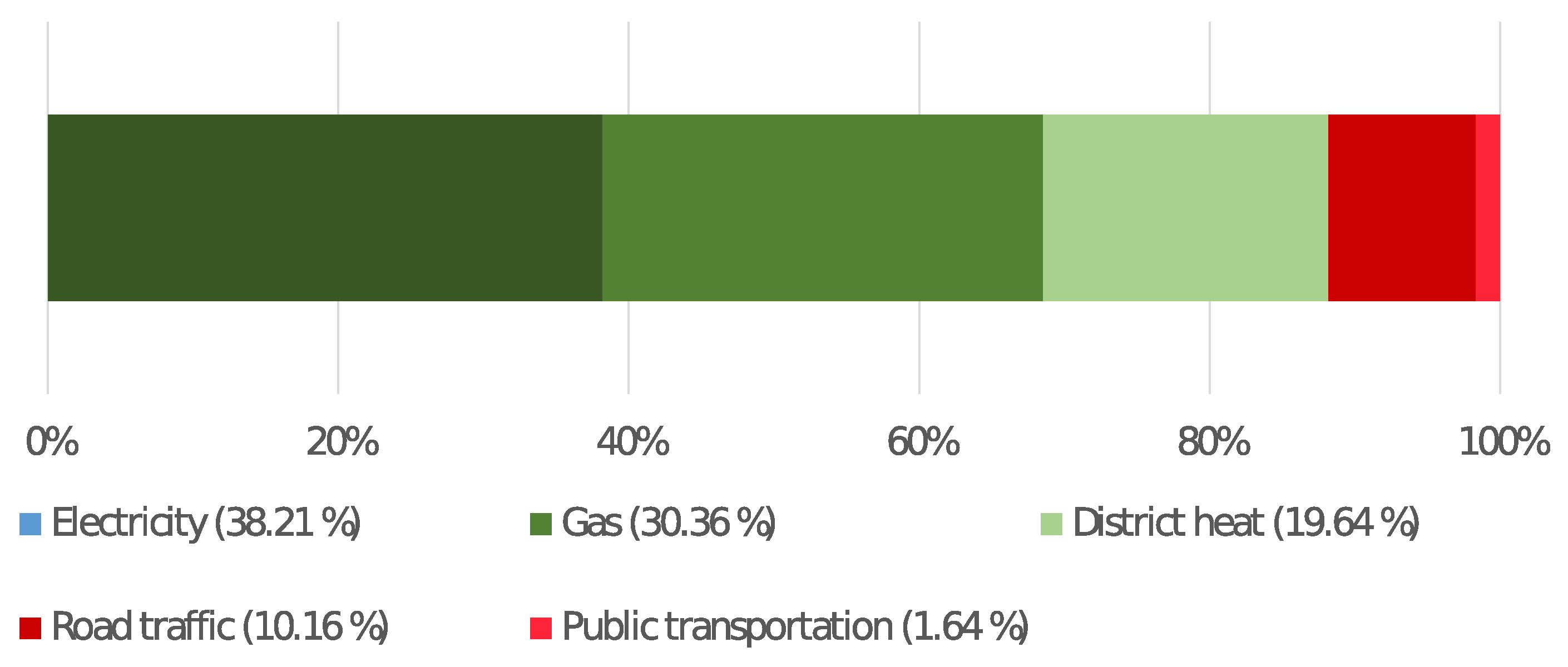
3.1. Territorial-Based Carbon Accounting

The territorial-based carbon emissions were grouped into the stationary and the traffic sectors. First, the results of the stationary sector are shown.

Table 1. Total energy consumption of the stationary sector for different zip codes in Wedding in 2016. Figure S1 in the Supplementary Materials shows a map of Wedding and its zip codes.

Zip Code	Share of Area in Wedding [%]	District Heat Consumption Wedding [GWh]	Natural Gas Consumption Wedding [GWh]	Electricity Consumption Wedding [GWh]
13347	86	83.9	48.4	54.6
13349	100	23.8	49.4	31.1
13351	100	37.5	31.3	21.3
13353	100	148.7	328.2	146.6
13359	2	0.1	2.0	0.8
13405	1.8	4.3	15.2	13.8
13407	6	1.1	16.9	7.7
13409	1	0.1	1.4	0.6
Total		299.4	492.8	276.5

shows the total energy consumption of these different sectors for the zip codes in Wedding in the year 2016. Additionally, the part of energy consumption used in Wedding is displayed. The highest energy consumption in all sectors occurs in zip code area 13,353. The total share of energy consumption was under 8% for the zip codes 13,359, 13,405, 13,407, and 13,409 compared to the total energy consumption of Wedding.

Around ¾ of the energy consumption was related to the heat supply (district heat and gas) and only ¼ could be attributed to electricity. The natural gas consumption contributed more than half to the total energy consumption.

The resulting carbon emissions of the energy consumption are shown in

Table 2. Energy consumption and resulting carbon emissions for the stationary sector.

	District Heat	Natural Gas	Electricity
Energy consumption [GWh]	299.4	492.8	276.5
Emission factor [t CO2-eq/MWh]	0.26	0.25	0.55
CO2-eq. [t]	78,741.1	121,722.3	153,187.3

.

Whereas electricity is responsible for only a quarter of the overall energy consumption, it amounts to almost half of the CO₂-eq emissions. Natural gas, which accounts for almost half of the energy consumption, was, with 35%, the second-largest emitter of CO₂-eq. emissions. Overall, the stationary sector of Wedding was annually responsible for 353,651 t CO₂-eq., which translates to 4.07 t CO₂-eq. per person and year.

In the following, the CO₂-eq. of the transport sector (divided into road transport and local public transport) are outlined. From the last traffic census of Berlin carried out in 2014, daily average traffic volumes for streets in Wedding were exported. Table S4 in the Supplementary Materials shows the main roads in Wedding, their length, and their average traffic intensity. The most frequented roads in Wedding are Müllerstraße and Seestraße. These are also the longest road sections in the urban district.

Table 3. Vehicle kilometers, energy consumption, and carbon emissions of road traffic in Wedding for 2014.

	Vehicle-km per Day (Tkm)	Vehicle-km per Year (Tkm)	Final Energy Consumption (GWh)	CO2-eq. Emissions (t)
Cars	346	126,122	99	30,328
Trucks > 3.5 t	13	4627	13	3908
Delivery vans ≤ 3.5 t	42	15,459	13	3932
Buses	3	1191	5	1646
Coaches	1	422	2	541
Motorcycles	10	3741	1	370
Total	415	151,562	132	40,724

shows the vehicle kilometers per year, the final energy consumption, and the annual CO₂-eq emissions. Both final energy consumption and CO₂-eq. emissions were calculated with emission factors (Table S1 in the Supplementary Materials).

The road traffic was responsible for 40,724 t CO₂-eq/a. The vehicle that contributed most to CO₂-eq. emissions was the car, followed by trucks and delivery vans. The highest vehicle kilometers were also driven with cars, followed by delivery vans and motorcycles; therefore, there is a correlation between driven kilometers and CO₂-eq.

Since the emission factors for local public transport refer to seat kilometers, the traffic volume had to be determined in this unit.

Table 4. Seat kilometers, energy consumption, and carbon emissions of public transport in Wedding.

	Seat Kilometers per Year (Tkm)	Energy Consumption (GWh/a)	CO2-eq (t/a)
Urban Railway	82,047	1.66	998
Metro 6	299,065	6.06	3637
Metro 9	137,014	2.78	1666
Tram M13	14,367	0.29	175
Tram 50	7855	0.16	96
Total	540,348	10.95	6572

shows the means of transport, the annual seat kilometers, and the annual CO₂-eq. emissions of public transport.

Because of the local public transport, 6571 tons of CO₂-eq per year are emitted annually in Wedding. The highest emissions are caused by metro line 6, whereas tramline 50 emits the least CO₂, which also have the highest and lowest seat kilometers per year, respectively.

The results of the territorial-based footprint are summarized in Table S5 in the Supplementary Materials, where the energy consumption and corresponding CO₂-eq. emissions of the stationary and transport sectors are listed. The largest emissions result from the stationary sector. This was followed by road traffic, whereas local public transport had the lowest emissions. Altogether, 400,947 tons of CO₂-eq. emissions are emitted in the district of Wedding per year. This corresponds to 4.61 tons of carbon emissions per person per year. Figure 2 is a visual presentation of the distribution of these CO₂-eq. emissions showing that 88% of the emissions can be attributed to the stationary sector and 10% to road traffic.

Only 2% of the emissions can be assigned to public transport. Heat (district heating and natural gas) accounted for the largest share of emissions (50%), followed by electricity with 38% and traffic with 12% of the total emissions.

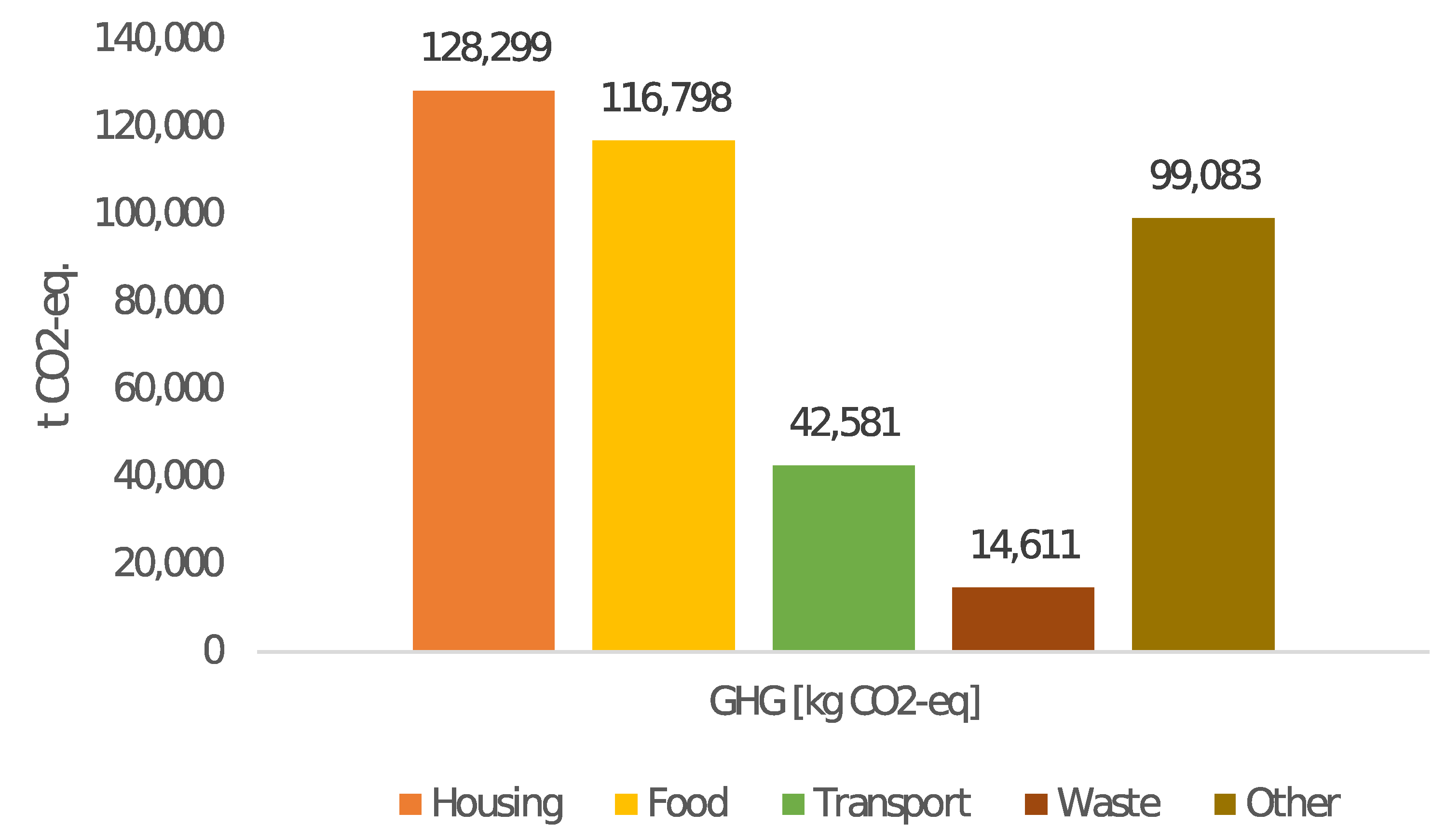
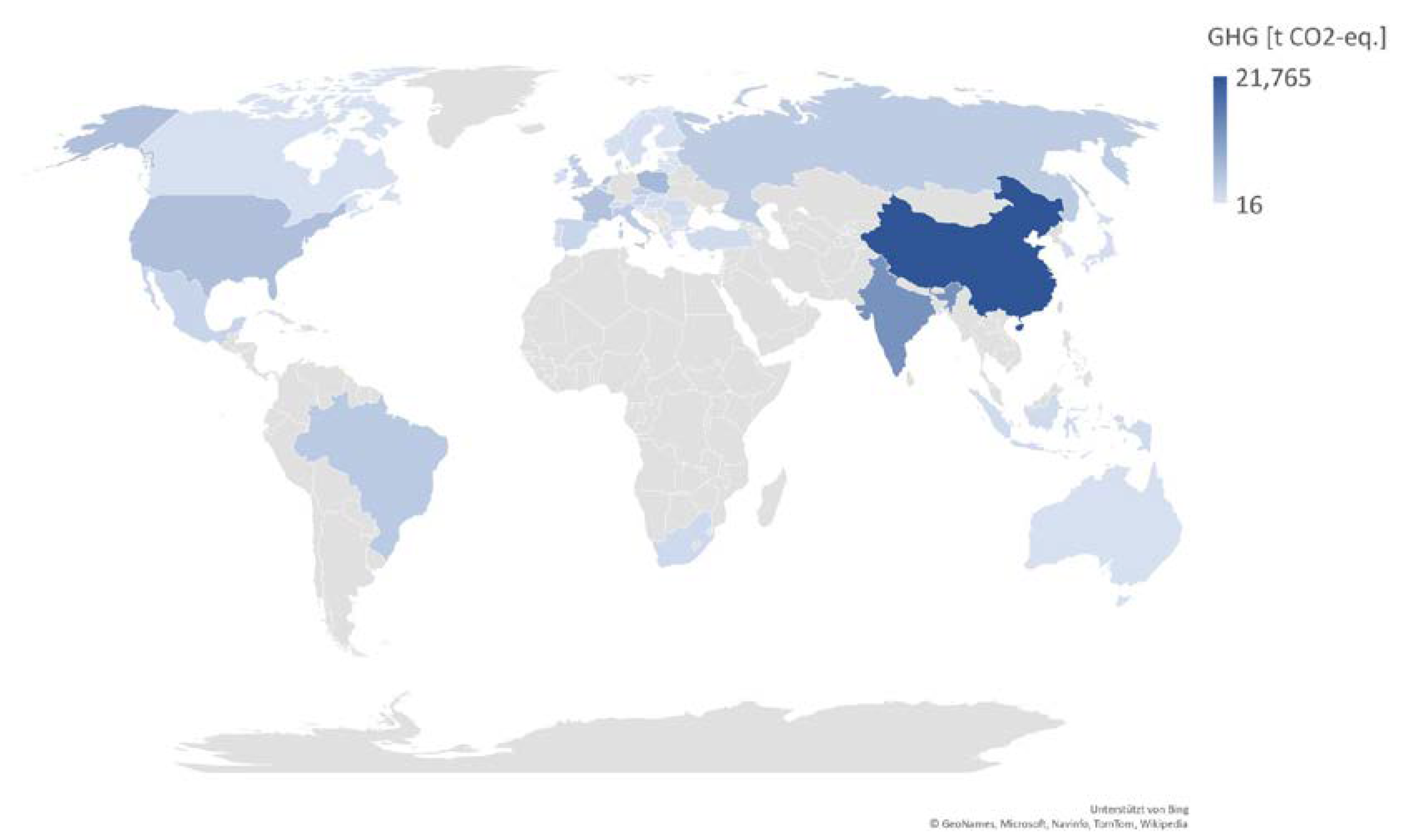
3.2. Consumption-Based Carbon Accounting

In the following section, the results of the input–output calculations for the calculation of the consumption-based carbon emissions of Wedding are presented. In total, the CO₂-eq. emissions due to the consumption of the people living in Wedding is 401,371 t per year.

Table 5. Overview of CO₂-eq. emissions of the ten sectors with the highest emissions.

CO2 (t CO2-eq.)				CH4 (t CO2-eq.)				N2O (t CO2-eq.)
Sector	CO2	Total GHG	Share (%)	Sector	CH4	Total GHG	Share (%)	Sector	N2O	Total GHG	Share (%)
Real estate services	31,583	33,960	93	Animal products	14,723	23,126	64	Wheat	5749	8387	69
Steam and hot water supply services	22,116	22,605	98	Crops	11,002	18,051	61	Cereal grains	5030	7421	68
Electricity by coal	18,243	18,924	96	Leather and leather products	7678	12,717	60	Animal products	4834	23,126	21
Chemicals	10,329	12,971	80	Products of meat cattle	6065	9149	66	Crops	3387	18,051	19
Hotel and restaurant services	8882	12,237	73	Processed rice	4136	6931	60	Products of meat cattle	2091	9149	23
Ceramic goods	8528	9595	89	Meat animals	4115	6150	67	Meat animals	1352	6150	22
Rubber and plastic products	6827	7505	91	Other Bituminous Coal	3804	7995	48	Hotel and restaurant services	1027	12,237	8
Other transport equipment	5098	5776	88	Dairy products	3591	7237	50	Vegetables, fruit, nuts	979	4886	20
Motor vehicles, trailers, and semi-trailers	5011	5610	89	Raw milk	3033	4201	72	Leather and leather products	970	12,717	8
Textiles	4722	6027	78	Hotel and restaurant services	2328	12,237	19	Dairy products	946	7237	13
Rest	153473	266161	58	Rest	30,136	293,577	10	Rest	9581	292,010	3
Total	274,814	401,371		Total	90,611	401,371		Total	35,946	401,371

lists the ten sectors with the CO₂ eq. emissions, sorted by the highest emissions in each sector. The full table can be found in Table S6 in the Supplementary Materials. Considering the three considered GHGs, CO₂ emissions had the largest share with 68%, followed by CH₄ with 23%, and N₂O with 9%.

In the case of CO₂-eq., the largest share was attributed to real estate services, followed by steam and hot water supply services. The third highest CO₂ emissions were caused by electricity supplied by coal. All three sectors can be roughly assigned to the sector “housing.” The largest emitters of CH₄ emissions are animal products, crops, and leather and leather products. Animal products and leather and leather products as well as the products of meat cattle, meat animals, dairy products, and raw milk are all sectors of animal husbandry. In terms of N₂O emissions, wheat, cereal grains, and animal products are the sectors with the highest emissions. Five of the ten sectors can be assigned to animal husbandry and four to agriculture. Among the top ten emitters considering all GHG emissions are hotel and restaurant services. The sectors with the highest CO₂-emissions were not as relevant for the other GHGs (CH₄ and N₂O). For the sectors with high CH₄ and N₂O emissions, overlaps occur. In Figure 3, the emissions of the greenhouse gases CO₂, CH₄, N₂O, are shown in CO₂-equivalents disaggregated by sector.

It is apparent that the three GHGs had their highest emissions in different sectors. For example, CO₂ emissions occurred most frequently for the housing sector (42%), whereas CH₄ emissions occurred most frequently in the food sector (76%). The hotspot of N₂O emissions, where 90% of the emissions occurred, was the food sector as well. Thirteen percent of the CO₂ emissions arose in the transport sector. CH₄ also had a 9% share in the transport sector, whereas N₂O only had a 1% share in this sector.

In Figure 4 the results (in CO₂-eq. emissions) of the aggregated sectors based on the results presented in Figure 3 and Table 5 are shown.

The housing sector had the largest share of emissions with 32% due to emissions of the energy sector as well as related to real estate services (rent). With 29.1% of the emissions, food had the second highest emissions. The transport sector was responsible for 10.6% of the total emissions because of private and public transport. With 3.6%, the waste sector follows, in which all sectors connected to the treatment of waste are summarized. The category “other,” in which 24.7% of the emissions occurred, is a collecting category for all sectors that could not be clearly assigned to any of the four other sectors, e.g., business services or textiles.

Further, a geographical evaluation showing the emissions origin based on the production of consumed products is presented in Figure 5. The regions clustered as “rest of the world” as well as Germany (responsible for 61% of the emissions) were excluded to achieve a better visual differentiation between the countries. The GHG emissions of all countries can be found in Table S7 in the Supplementary Materials.

In Europe, 12% of the GHG emissions occur. Within Europe, the highest emissions are attributable to Germany (61%), whereas the second highest emissions can be assigned to Poland and the third highest to France. Sixteen percent of the GHG emissions are emitted in Asia and Pacific, with China contributing the most to the emissions with a total of 5% and India contributing with 3%. The “rest of the world” regions of Asia and the Pacific are responsible for 5%. Seven percent of the emissions are emitted in America (including South and North America). The United States contributes to the emissions with 1.4% and Brazil with 1%. The “rest of the world” region of America is responsible for 4%.

The emissions in China can be traced back to textile production with 32%, to the production of electronics and machines with 22%, and to the production of chemicals with 10%. In India, 57% of the emissions can be attributed to the leather and leather products sector. Twenty-five percent of the emissions are attributable to the agricultural products crops and rice. In the United States, 35% of the emissions are generated by the production of chemicals and 10% by the aggregated food category (6% of which is meat). Transport also accounts for 15% of the emissions. In Poland, 36% of the emissions are related to coal and 19% to food production. The production of chemicals also plays a role with 7%. In France, no sector outweighs all others.

3.3. Comparison of the Approaches

The total carbon emissions of the two approaches revealed almost identical results and differed by only 424 t CO₂-eq/a and therefore by 0.11%.

The literature proposes that consumption-based carbon footprints tend to be higher than territorial-based ones in countries such as Germany that are net-importers of carbon emissions [44]. This proposal cannot be proven with this case study. With about 4.62 t CO₂-eq per person per year, the footprints are basically the same. The fact that the territorial-based footprint was not lower in this case study is mainly because of the energy consumption of Bayer Pharma AG, which most likely accounts for a large share of energy consumption.

Within the territorial-based results, 50% of the emissions occur because of heat, 38% because of electricity, and 12% because of transport. The classification is different in the consumption-based approach, as energy consumption is considered within the housing sector, which accounts for only 32% of the emissions. Similarities can be found in the traffic and transportation sectors. Eleven percent of the consumption-based emissions can be attributed to the transport sector. The food sector, which represents 29% of the emissions, was not included in the territorial-based approach. Since there is no airport within the boundaries of the Wedding district, emissions from air traffic were not included in the territorial-based approach. However, in the consumption-based approach, they are taken into account but still lead to lower results. Therefore, it is close to certain that the consumption-based approach underestimates emissions due to housing and transport. One reason for this might be economic allocation in environmentally extended input–output analysis. This will lead to the allocation that two people that live in the same flat would obtain an allocation of emissions based on their rent, so that people that pay more rent would obtain a higher share of emissions. Additionally, transport emissions in the Wedding district do not exclusively occur because of the mobility of its own residents. The consumption-based approach only assesses the impact of the mobility of the local residents, whereas the territorial-based approach also accounts for traffic that leads through the relatively central district of Wedding, which people from the suburbs have to cross to commute to work. Additionally, in Berlin, few people own a car (381.8 per 1000 inhabitants) with an even lower number in Wedding (255 per 1000 inhabitants). These differing system boundaries might explain some of the differences [45].

The results of the territorial-based approach suggest that reduction potentials in Wedding occur especially in the area of heat. This could be achieved above all with energetic renovation and education of citizens to increase the efficiency of heat use.

In the consumption-based approach, besides the housing sector, which can be represented much more realistically by the territorial-based approach, the food sector is a hotspot. When developing strategies and actions to reduce carbon emissions, this sector should be in focus on the local level. Examples of such actions would be citizen dialogues on nutrition or action days on climate-friendly nutrition in schools, reduction of food waste, and food sharing.

In

Table 6. Comparison of the approaches.

	Territorial-Based Approach		Consumption-Based Approach
	Weaknesses	Strengths	Weaknesses	Strengths
Applicability	Local data for energy consumption and traffic needed	Simple calculations with emission factors	Consumption expenditure data necessary; some advanced mathematics needed	Differentiation of CO2, CH4, N2O
Availability of data	Data from different years	Specific data available for Wedding	No local data available	Global IO data with emission factors
Reproducibility	Calculation tool is not open source; several standards	Reproduction was possible based on publication by Hertele et al. [28]	No standardization of calculation
Relevance of results	Only final energy consumption is considered	Data is available on site; therefore, results can lead to action in Wedding by local government	Relevance equivalent to resolution of CES data	Results focus on people’s consumption and might change consumption patterns

, the two accounting approaches are compared regarding their weaknesses and strengths using the criteria: applicability, availability of data, and reproducibility and relevance of results, as outlined in Section 2.3.

Table 6 shows that both approaches for calculating a district’s carbon footprint have strengths and weaknesses for the analyzed criteria. Depending on the perspective, one method can be preferred over the other. For instance, the consumption-based approach enables the disaggregation of different greenhouse gases, which facilitates the identification of tailored reduction measures. Technologies and measures to reduce greenhouse gas emissions are often emission-specific: for laughing gas, the reduction of mineral nitrogen fertilizer use will reduce emissions, whereas, for carbon emissions, gains in efficiency and renewable technologies will be the best measures to reduce emissions. If, for example, a carbon footprint is calculated in order to detect hotspots in the district and take action, the territorial-based approach would clearly be preferable, since site-specific data is used. If, on the other hand, residents are to be made aware of the impacts that their consumption have on global warming, the consumption-based approach would be the better choice.

4. Discussion

In the following, the application of the methods and applied data (see Section 4.1) and the results (see Section 4.2) are discussed.

4.1. Discussion of Application of Methods and Used Data Sources

In order to calculate the territorial carbon emissions, local energy and traffic data provided by the State of Berlin were used. The energy data is available on the level of districts and postal codes. The district of Wedding cannot be delimited by the boundaries of the postal code areas. Therefore, the postal codes within the area were scaled by their percentage share, which may lead to non-real energy consumption data. Furthermore, some energy sources were neglected because of statements of the district chimney sweeps (fuel oil, biomass).

In the context of the collection of traffic data, only the main roads in Wedding were considered. It is unclear what influence the secondary road network has on emissions from the transport sector.

Within the transport sector, the emissions caused by buses were calculated. This was done using the traffic volume data. As a sensitivity analysis, traffic volumes were calculated with the help of timetables, as it was done for other public transport vehicles. This resulted in 883 t CO₂-eq. emissions, only half of the emissions compared to the traffic volume data. The emissions resulting from the traffic volume data were used for the evaluation for a conservative estimate.

The data for energy consumption was from 2016 and the traffic data from 2014, so data from different years were added together. Furthermore, the data was already four or six years old and therefore cannot reflect the status of the urban district. Because of this inconsistent data situation, the results may be affected.

For the consumption-based approach, a final demand vector is necessary to use input–output tables for the calculation of environmental impacts. Since there was no specific consumption data for Wedding, Berlin, the CES data of the city of Berlin was used. These were then scaled to the inhabitants of Wedding using socio-economic comparisons. It was assumed that Mitte and Wedding have the same distribution of household sizes. However, the ratio of household sizes in Wedding may differ from that in Mitte. In Mitte, many young people and students live in small apartments, whereas Wedding could be described as a family district with larger household sizes. Depending on the household size, the consumption data differed and therefore the consumption of the residents in Wedding was only assumed and could not be represented properly. A survey on consumer expenditure in Wedding could have led to results that are more meaningful.

As part of the consumption-based calculation, a correspondence table had to be created first, as described in the methods section, to convert the CES data into Exiobase sectors. However, since Exiobase sectors are not reflected one-to-one in the CES consumption categories, some Exiobase sectors were assigned to several CES consumption categories. The correspondence table had to be normalized for the IO calculations. The assumption that Germany and the urban district Wedding share the same final demand structure is possibly also not correct. According to Engel’s law [46], households with lower incomes spend proportionally more money on food, and Wedding, compared to Germany, has a significantly lower income rate. The average income per household in Wedding is EUR 1850 per month and household with 30.7% of people receiving unemployment benefit II (Hartz 4) and thus is significantly lower compared to EUR 2025 per month and household in Berlin and EUR 3661 per month and household in all of Germany [47,48].

Because of a lack of proper criteria available in the literature concerning the carbon accounting of cities to compare different approaches, the comparison was done using a juxtaposition of weaknesses and strengths. It would be conceivable to carry out the comparison by means of a criteria catalogue. However, because a case study was conducted, the advantages and disadvantages of the two approaches could be identified directly during the implementation.

Further, the validity of the consumption-based approach results was low, as no local consumption data was available. To avoid this problem, it is recommended to first conduct a survey on consumption at the local level, if no specific consumption data is available, to obtain results that are more specific. When studies with the territorial-based approach are conducted at the local level, it should be considered to emphasize in the presentation of the results that the consumption of products leads to carbon emissions in the supply chain. Especially in the area of food production, this should be pointed out.

In order to be able to make statements about which approach of carbon accounting is preferable over the other to calculate emissions on a district level, it is recommended to carry out further comparative studies. This should be done on the level of urban districts but also of whole cities. Furthermore, the method of the consumption-based approach should be further standardized to achieve comparable results.

4.2. Discussion of Limitations of Case Study Results

First, the territorial-based accounting results of the case study are discussed. As described in the method section, some energy sources were neglected. For example, heating oil was neglected because of statements of a chimney sweeper in the sweeping district of Wedding. In a comparable study, which concentrated on the Berlin district of Charlottenburg-Wilmersdorf, 16% of the carbon emissions in the stationary area were due to the consumption of fuel oil [49]. In a sensitivity analysis, 16% of the carbon emissions were added to the stationary emission result in Wedding. Instead of 353,651 t CO₂ eq. emissions in the stationary area, 410,235 t CO₂-eq. emissions would be emitted. The total emissions in the district would increase to 457,531 t CO₂-eq., which is an increase of 12%. However, in Germany, most single-family houses are heated with heating oil. In Charlottenburg-Wilmersdorf, there are some settlements with single-family houses, which would explain the higher proportion of heating oil. This is also evident in the map of the settlement structure [50]. In the postal code areas 14193 (urban district Dahlem) and 14055 (Westend), the predominant residential use is characterized by single-family homes. There is no area with this type of residential use in Wedding.

As shown in Figure 2, about ¾ of the final energy consumption is allocated to heat supply and ¼ to electricity use. This does not correspond to the average values on a national German level. According to the Federal Environment Agency, heat accounts for just over 50% of the final energy consumption in Germany [51]. The difference for Wedding, Berlin might be due to the fact that few buildings have been energetically renovated, but a large part of the development is characterized by old buildings. In Wedding, most buildings were built before 1930 [52]. Natural gas alone is responsible for half of the energy consumption and is commonly used in unrenovated houses. Low renovation rates in Wedding might therefore explain the high consumption of natural gas.

In relation to the number of inhabitants, the emissions from road traffic are rather low and amount to 0.5 t CO₂-eq per person. In the comparative study from Charlottenburg-Wilmersdorf, emissions were more than twice as high at 1.3 t CO₂-eq per person [49]. This was mainly because one of the most frequented roads in Berlin leads through Charlottenburg-Wilmersdorf. The almost 10-km long section of the A100, a six-lane highway, has a traffic volume of up to 100,000 vehicles per day. Such a route is not located in Wedding [35]. Additionally, Weeding has a higher population density compared to Charlottenburg-Wilmersdorf, which might be responsible for less traffic per capita.

Figure 2 summarizes the territorial results. In total, 88% of the carbon emissions can be attributed to the stationary sector, whereas only 10% of the emissions occur in road traffic and 2% in public transport. The State Statistical Office in Berlin publishes an annual CO₂ balance for Berlin. The most recent balance, from 2017, indicates that 64.6% of the emissions are attributable to the sector “households, trade, commerce and services and other consumers,” 29.3% to transport, and 6.1% to the extraction of stone and earth, other mining and manufacturing industries” [53]. If the last sector, which does not play a role in this study, is excluded from the calculation, 31% is attributable to the transport sector and 69% to the sector “households, trades, commerce and services and other consumers.” The energy consumption in Berlin is assigned to this sector. In Wedding, the emissions associated with energy consumption are around 20% higher than the Berlin average and the traffic emissions are correspondingly 20% lower. In the comparable study for the district of Charlottenburg-Wilmersdorf, the emissions for the stationary sector are also almost 70% and for the transport sector 30%. One explanation for these differences may be a reduced energy consumption for traffic in Wedding, which is due to the high population density. Charlottenburg-Wilmersdorf has a population density of 5235 people per square kilometer, whereas Wedding has a population density of 9405 people per square kilometer, which is almost twice as high. All of Berlin has a population density of 4090 people per square kilometer. A lower proportion of carbon emissions in the traffic sector is therefore mostly due to lower emissions related to transport that supposedly correlates with population density [54,55]. Angel et al. [55] propose that the shape compactness of a city influences the GHG emissions in a city, though this factor was not part of this study.

In

Table 7. Comparison of obtained results with other studies.

Publication	Emissions per Capita (t-CO2-eq)	Geographical Focus	Supposed Reason for Difference in Result	Consumption- or Territorial-Based
This study	4.61	Wedding	/	Territorial
This study	4.62	Wedding	/	Consumption
[56]	7.07	Charlottenburg Wilmersdorf	Different urban form	Territorial
[42]	8.9	Berlin	Different databases, lower income of people in Wedding, and larger household sizes	Consumption
[57]	13.7	Berlin	Different databases, lower income of people in Wedding, and larger household sizes	Consumption
[58]	11.63	Germany	Lower income in Wedding, less densely populated, lower heating demand in all of Germany because of better energetic renovation rate	Territorial

, the results of this study are compared to other studies that calculated GHG emissions within a specific area, and the supposed reasons for differences are displayed.

If consumption-based emissions per capita in Wedding are considered, these amount to approximately 4.62 t CO₂-eq per year. The average German citizen emits a total of 11.63 t CO₂-eq per year, which is more than twice as much as one person in Wedding [58]. Pichler et al. [28] calculated, among others, a carbon footprint for Berlin, resulting annually in 8.9 t CO₂-eq per person. Even higher is the carbon footprint Ivanova et al. [57] calculated for Berlin, which, annually, is 13.7 t CO₂-eq per person. These high differences are probably due to different databases. This study and the calculations from Pichler et al. [42] use the same expenditure data, but different IO models were used. Ivanova et al. [57] used Exiobase but different consumption data. The conversion rates from purchaser to base prices have not been published and are probably diverse among the different studies. As mentioned before, people in Wedding have a lower average income than in Berlin and Germany. Kovács et al. [59] also found that lower consumption lowers the environmental footprint. Another reason why the consumption-based results in the study are lower than those calculated by Pichler et al. [42] and Ivanova et al. [57] is the economic allocation of IO calculations. If people have a similar flat, but pay different rents, different emissions are assigned. In Wedding, the rents are, compared to Berlin, rather low because the residential area is categorized as simple [60], which might have led to an underestimation of emissions with economic allocation.

A way forward could be the Organizational LCA approach, which has been recently adapted to cities [61], as it includes upstream and downstream emissions. Additionally, it set up a city structure to highlight which activities and respective emission levels can be influenced by the local government. Furthermore, it includes several environmental impacts and thus reduces the risk of shifts of burden from carbon emissions to other impacts if measures to reduce carbon emissions are taken [62].

5. Conclusions

This study performed a territorial- and consumption-based carbon footprint for the Wedding district in Berlin. The footprint resulted in 400,947 tons of CO₂-eq. emissions per year for the territorial approach and in 401,371 t per year for the consumption-based approach, which results in 4.61 t CO₂-eq and 4.62 t CO₂-eq per capita, respectively. The highest shares of CO₂-eq. emissions in both approaches were related to the housing, heating, and electricity sector. However, the consumption-based approach also calculated a high share of emissions in the food sector that the territorial approach neglected. As the results are quite similar, this study cannot verify that the consumption-based approach mostly leads to higher emissions per capita in the Global North. The results are rather low compared to other conducted studies, which might be because Wedding is a comparatively poor urban district with a high population density and a relatively high share of multiple-person households. Strengths and weaknesses of the consumption- and territorial-based approach could be derived, for example, that the territorial approach is more suitable to derive measures for local climate action, whereas the consumption-based approach highlights the responsibility of consumers for GHG emissions along the supply chain and the importance of the food sector. Thus, the territorial-based approach identifies emissions related to urban form, whereas the consumption-based approach underlines the impact of food production and animal products and thus consumption lifestyles.

References

1. United Nations Development Programme Goal 11: Sustainable Cities and Communities. Available online: https://www.undp.org/content/undp/en/home/sustainable-development-goals/goal-11-sustainable-cities-and-communities.html (accessed on 28 September 2020).
2. Grimm, N.B.; Faeth, S.H.; Golubiewski, N.E.; Redman, C.L.; Wu, J.; Bai, X.; Briggs, J.M. Global change and the ecology of cities. Science 2008, 319, 756–760. [Google Scholar] [CrossRef] [PubMed] [Green Version]
3. Rosenzweig, C.; Solecki, W.; Hammer, S.A.; Mehrotra, S. Cities lead the way in climate–change action. Nature 2010, 467, 909–911. [Google Scholar] [CrossRef] [PubMed]
4. British Standards Institution. PAS 2070 specification for the assessment of greenhouse gas emissions of a city. In Direct Plus Supply Chain and Consumption-Based Methodologies; BSI Standards Limited: London, UK, 2013; ISBN 978-0-580-77402-7. [Google Scholar]
5. WRI. C40—ICLEI Global Protocol for Community-Scale Greenhouse Gas Emission Inventories. An Accounting and Reporting Standard for Cities; WRI: Washington, DC, USA, 2014; ISBN 1-56973-846-7. [Google Scholar]
6. IPCC. 2006 IPCC Guidelines for National Greenhouse Gas Inventories Volume 1 General Guidance and Reporting; IPCC: Geneva, Switzerland, 2006. [Google Scholar]
7. Chen, G.; Shan, Y.; Hu, Y.; Tong, K.; Wiedmann, T.; Ramaswami, A.; Guan, D.; Shi, L.; Wang, Y. Review on City-Level Carbon Accounting. Environ. Sci. Technol. 2019, 53, 5545–5558. [Google Scholar] [CrossRef] [PubMed]
8. Lombardi, M.; Laiola, E.; Tricase, C.; Rana, R. Assessing the Urban Carbon Footprint: An Overview. Environ. Impact Assess. Rev. 2017, 66, 43–52. [Google Scholar] [CrossRef]
9. WBCSD. WRI The Greenhouse Gas Protocol—A Corporate Accounting and Reporting Standard (Revised Edition); WBCSD: Geneva, Switzerland, 2004; p. 116. [Google Scholar]
10. Chen, S.; Long, H.; Chen, B.; Feng, K.; Hubacek, K. Urban Carbon Footprints across Scale: Important Considerations for Choosing System Boundaries. Appl. Energy 2020, 259, 114201. [Google Scholar] [CrossRef]
11. Arioli, M.S.; D’Agosto, M.A.; Amaral, F.G.; Cybis, H.B.B. The evolution of city-scale GHG emissions inventory methods: A systematic review. Environ. Impact Assess. Rev. 2020, 80, 106316. [Google Scholar] [CrossRef]
12. Athanassiadis, A.; Christis, M.; Bouillard, P.; Vercalsteren, A.; Crawford, R.H.; Khan, A.Z. Comparing a territorial-based and a consumption-based approach to assess the local and global environmental performance of cities. J. Clean. Prod. 2018, 173, 112–123. [Google Scholar] [CrossRef]
13. Fan, J.-L.; Hou, Y.-B.; Wang, Q.; Wang, C.; Wei, Y.-M. Exploring the characteristics of production-based and consumption-based carbon emissions of major economies: A multiple-dimension comparison. Appl. Energy 2016, 184, 790–799. [Google Scholar] [CrossRef]
14. Bastianoni, S.; Pulselli, F.M.; Tiezzi, E. The problem of assigning responsibility for greenhouse gas emissions. Ecol. Econ. 2004, 49, 253–257. [Google Scholar] [CrossRef]
15. Boitier, B. CO2 Emissions Production-Based Accounting vs Consumption: Insights from the WIOD Databases. 2012. Available online: http://www.wiod.org/conferences/groningen/paper_Boitier.pdf (accessed on 28 June 2021).
16. Li, Y.; Hewitt, C.N. The Effect of Trade between China and the UK on National and Global Carbon Dioxide Emissions. Energy Policy 2008, 36, 1907–1914. [Google Scholar] [CrossRef]
17. Peters, G.P. From production-based to consumption-based national emission inventories. Ecol. Econ. 2008, 65, 13–23. [Google Scholar] [CrossRef]
18. Peters, G.P.; Hertwich, E.G. Post-kyoto greenhouse gas inventories: Production versus consumption. Clim. Chang. 2008, 86, 51–66. [Google Scholar] [CrossRef]
19. Zhang, Q.; Fang, K. Comment on “Consumption-Based versus Production-Based Accounting of CO2 Emissions: Is There Evidence for Carbon Leakage?”. Environ. Sci. Policy 2019, 101, 94–96. [Google Scholar] [CrossRef]
20. Caro, D.; Bastianoni, S.; Borghesi, S.; Pulselli, F.M. On the Feasibility of a Consumer-Based Allocation Method in National GHG Inventories. Ecol. Indic. 2014, 36, 640–643. [Google Scholar] [CrossRef]
21. Wang, X.; Zheng, H.; Wang, Z.; Shan, Y.; Meng, J.; Liang, X.; Feng, K.; Guan, D. Kazakhstan’s CO2 Emissions in the Post-Kyoto Protocol Era: Production- and Consumption-Based Analysis. J. Environ. Manag. 2019, 249, 109393. [Google Scholar] [CrossRef] [Green Version]
22. Harris, S.; Weinzettel, J.; Bigano, A.; Källmén, A. Low Carbon Cities in 2050? GHG Emissions of European Cities Using Production-Based and Consumption-Based Emission Accounting Methods. J. Clean. Prod. 2019, 119206. [Google Scholar] [CrossRef]
23. Liu, L.; Qu, J.; Maraseni, T.N.; Niu, Y.; Zeng, J.; Zhang, L.; Xu, L. Household CO2 Emissions: Current Status and Future Perspectives. IJERPH 2020, 17, 7077. [Google Scholar] [CrossRef]
24. Bakó, F.; Berkes, J.; Szigeti, C. Households’ Electricity Consumption in Hungarian Urban Areas. Energies 2021, 14, 2899. [Google Scholar] [CrossRef]
25. Amt für Statistik Berlin-Brandenburg Einwohnerinnen und Einwohner im Land Berlin am 31. December 2018, p. 38. Available online: https://statistik-berlin-brandenburg.de/publikationen/stat_berichte/2019/SB_A01-16-00_2018h02_BE.pdf (accessed on 28 June 2021).
26. Land Berlin Wedding. Available online: http://wedding.berndschimmler.de/index.html (accessed on 9 May 2020).
27. Hermannsson, K.; McIntyre, S.G. Local Consumption and Territorial Based Accounting for CO2 Emissions. Ecol. Econ. 2014, 104, 1–11. [Google Scholar] [CrossRef] [Green Version]
28. Hertle, H.; Dünnebeil, F.; Gebauer, C.; Gugel, B.; Heuer, C.; Kutzner, F.; Vogt, R. Empfehlungen zur Methodik der Kommunalen Treibhausgas- Bilanzierung für den Energie- und Verkehrssektor in Deutschland; Institut für Energie: Leipzig, Germany, 2014; p. 103. [Google Scholar]
29. ICLEI HEAT—Harmonized Emissions Analysis Tool. Available online: https://ledsgp.org/wp-content/uploads/2015/09/HEATplus_brochure.pdf (accessed on 6 October 2020).
30. ICLEI Clean Air Climate Protection Software. Available online: http://www.4cleanair.org/Oldmembers/members/committee/ozone/webcastSIslides.pdf (accessed on 6 October 2020).
31. Hertle, H.; Dünnebeil, F.; Gugel, B.; Rechsteiner, E.; Reinhard, C. Empfehlungen zur Methodik der Kommunalen Treibhausgasbilanzierung für den Energie- und Verkehrssektor in Deutschland Kurzfassung (Aktualisierung 11/2019); ifeu: Heidelberg, Germany, 2019. [Google Scholar]
32. Allekotte, M.; Biemann, K.; Heidt, C.; Colson, M.; Knörr, W. Aktualisierung der Modelle TREMOD/TREMOD-MM für die Emissionsberichterstattung 2020 (Berichtsperiode 1990–2018); Umweltbundesamt: Vienna, Austria, 2020; p. 205. [Google Scholar]
33. Diekelmann, P. Klimaschutz in Kommunen: Praxisleitfaden; Deutsches Institut für Urbanistik, Institut für Energie- und Umweltforschung, Klima-Bündnis Europäischer Städte mit den Indigenen Völkern der Regenwälder zum Erhalt der Erdatmosphäre, Eds.; Service & Kompetenzzentrum Kommunaler Klimaschutz, SK:KK; 3. aktualisierte und erweiterte Auflage; Deutsches Institut für Urbanistik gGmbH: Berlin, Germany, 2018; ISBN 978-3-88118-585-1. [Google Scholar]
34. Senatsverwaltung für Wirtschaft, Energie und Betriebe Energieatlas Berlin. Available online: https://energieatlas.berlin.de/ (accessed on 1 May 2021).
35. Senatsverwaltung für Stadtentwicklung und Wohnen Umweltatlas Berlin/Verkehrsmengen. 2014. Available online: https://fbinter.stadt-berlin.de/fb/index.jsp?loginkey=zoomStart&mapId=wmsk_07_01verkmeng2014@senstadt&bbox=372260,5811257,399837,5825075 (accessed on 26 September 2020).
36. BVG FahrInfo und Linienverlauf. Available online: https://www.bvg.de/de/Fahrinfo (accessed on 1 May 2021).
37. S-Bahn Berlin GmbH Linienfahrpläne. Available online: https://sbahn.berlin/fahren/fahrplanauskunft/linienfahrplaene/ (accessed on 1 May 2021).
38. Soltani, M.; Rahmani, O.; Beiranvand Pour, A.; Ghaderpour, Y.; Ngah, I.; Misnan, S.H. Determinants of variation in household energy choice and consumption: Case from Mahabad City, Iran. Sustainability 2019, 11, 4775. [Google Scholar] [CrossRef] [Green Version]
39. Afionis, S.; Sakai, M.; Scott, K.; Barrett, J.; Gouldson, A. Consumption-Based Carbon Accounting: Does it have a future?: Consumption-Based Carbon Accounting. WIREs Clim. Chang. 2017, 8, e438. [Google Scholar] [CrossRef]
40. Amt für Statistik Berlin-Brandenburg Einkommen Und Einnahmen Sowie Ausgaben Privater Haushalte Im Land Berlin 2018 2020. Available online: https://cdn0.scrvt.com/ee046e2ad31b65165b1780ff8b3b5fb6/8a6de9bad2ecfdb7/a6beefca459a/SB_O02-03-00_2018j05_BE.pdf (accessed on 28 June 2021).
41. Stadler, K.; Wood, R.; Bulavskaya, T.; Södersten, C.-J.; Simas, M.; Schmidt, S.; Usubiaga, A.; Acosta-Fernández, J.; Kuenen, J.; Bruckner, M.; et al. EXIOBASE 3: Developing a time series of detailed environmentally extended multi-regional input-output tables: EXIOBASE 3. J. Ind. Ecol. 2018, 22, 502–515. [Google Scholar] [CrossRef] [Green Version]
42. Pichler, P.-P.; Zwickel, T.; Chavez, A.; Kretschmer, T.; Seddon, J.; Weisz, H. Reducing urban greenhouse gas footprints. Sci. Rep. 2017, 7, 14659. [Google Scholar] [CrossRef] [Green Version]
43. USEPA. Global Greenhouse Gas Emissions Data. Available online: https://www.epa.gov/ghgemissions/global-greenhouse-gas-emissions-data (accessed on 26 September 2020).
44. Davis, S.J.; Caldeira, K. Consumption-based accounting of CO2 emissions. Proc. Natl. Acad. Sci. USA 2010, 107, 5687–5692. [Google Scholar] [CrossRef] [Green Version]
45. Senatsverwaltung für Stadtentwicklung und Umwelt Schriftliche Anfrage Des Abgeordneten Gerwald Claus-Brunner (PIRATEN)—Aktueller Berliner Motorisierungsgrad 2015. Available online: https://kleineanfragen.de/berlin/17/16873-aktueller-berliner-motorisierungsgrad (accessed on 28 June 2021).
46. Engel, E. Die Productions-und Consumtionsverhältnisse des Königreichs Sachsen. In Zeitschrift des Statistischen Bureaus des Königlich Sächsischen Ministerium des Inneren; Forgotten Books: London, UK, 1857. [Google Scholar]
47. Bundeszentrale für Politische Bildung Einkommen privater Haushalte|bpb. Available online: https://www.bpb.de/nachschlagen/zahlen-und-fakten/soziale-situation-in-deutschland/61754/einkommen-privater-haushalte (accessed on 21 June 2021).
48. Bezirksamt Berlin Mitte Basisdaten Zur Bevölkerung Und Sozialen Lage Im Bezirk Berlin-Mitte 2018. Available online: https://digital.zlb.de/viewer/metadata/15698546/1/ (accessed on 28 June 2021).
49. Thöle, G.; Reitemeyer, F. Bezirkliche Treibhausgasbilanz nach BISKO für Charlottenburg-Wilmersdorf. Available online: https://www.berlin.de/ba-charlottenburg-wilmersdorf/verwaltung/aemter/umwelt-und-naturschutzamt/klimaschutz/artikel.712319.php (accessed on 24 September 2020).
50. Senatsverwaltung für Stadtentwicklung und Wohnen Geoportal Berlin/Siedlungsstruktur Wohnen—Bezirksregionen 2010. Available online: https://fbinter.stadt-berlin.de/fb/index.jsp?loginkey=zoomStart&mapId=k_siedlungsstruktur_bzr@senstadt&bbox=373148,5812836,400960,5826772 (accessed on 24 September 2020).
51. Umweltbundesamt Energieverbrauch für Fossile und Erneuerbare Wärme. Available online: https://www.umweltbundesamt.de/daten/energie/energieverbrauch-fuer-fossile-erneuerbare-waerme (accessed on 24 September 2020).
52. Senatsverwaltung für Stadtentwicklung und Wohnen Umweltatlas Berlin/Gebäudealter Der Wohnbebauung. Available online: https://fbinter.stadt-berlin.de/fb/index.jsp (accessed on 24 September 2020).
53. Amt für Statistik Berlin-Brandenburg Energie- und CO2-Bilanz in Berlin 2017. 2019, p. 40. Available online: https://www.statistik-berlin-brandenburg.de/publikationen/stat_berichte/2019/SB_E04-04-00_2017j01_BE.pdf (accessed on 28 June 2021).
54. Xu, C.; Haase, D.; Su, M.; Yang, Z. The Impact of Urban Compactness on Energy-Related Greenhouse Gas Emissions across EU Member States: Population Density vs Physical Compactness. Appl. Energy 2019, 254, 113671. [Google Scholar] [CrossRef]
55. Angel, S.; Arango Franco, S.; Liu, Y.; Blei, A.M. The Shape Compactness of Urban Footprints. Prog. Plan. 2020, 139, 100429. [Google Scholar] [CrossRef]
56. Reitemeyer, F. Erstellung Einer Treibhausgasbilanz Für Bezirke Und Vergleich Mit Einer Verbraucherbasierten Treibhausgasbilanz Mit Direkten Und Indirekten Emissionen 2019. Available online: https://www.berlin.de/ba-charlottenburg-wilmersdorf/verwaltung/aemter/umwelt-und-naturschutzamt/artikel.113003.php (accessed on 28 June 2021).
57. Ivanova, D.; Vita, G.; Steen-Olsen, K.; Stadler, K.; Melo, P.C.; Wood, R.; Hertwich, E.G. Mapping the Carbon Footprint of EU Regions. Environ. Res. Lett. 2017, 12, 054013. [Google Scholar] [CrossRef]
58. Bundesministerium für Umwelt, Naturschutz und nukleare Sicherheit Klimaschutz in Zahlen (2018)—Fakten, Trends und Impulse deutscher Klimapolitik. 2018, p. 72. Available online: https://www.bmu.de/fileadmin/Daten_BMU/Pools/Broschueren/klimaschutz_in_zahlen_2018_bf.pdf (accessed on 28 June 2021).
59. Kovács, Z.; Harangozó, G.; Szigeti, C.; Koppány, K.; Kondor, A.C.; Szabó, B. Measuring the Impacts of Suburbanization with Ecological Footprint Calculations. Cities 2020, 101, 102715. [Google Scholar] [CrossRef]
60. Senatsverwaltung für Stadtentwicklung und Wohnen Berliner Mietspiegel 2019. Available online: https://www.stadtentwicklung.berlin.de/download/mietspiegel2019/Broschuere_Mietspiegel2019.pdf (accessed on 28 June 2021).
61. Cremer, A.; Müller, K.; Berger, M.; Finkbeiner, M. A Framework for Environmental Decision Support in Cities Incorporating Organizational LCA. Int. J. Life Cycle Assess. 2020, 25, 2204–2216. [Google Scholar] [CrossRef]
62. Cremer, A.; Berger, M.; Müller, K.; Finkbeiner, M. The First City Organizational LCA Case Study: Feasibility and Lessons Learned from Vienna. Sustainability 2021, 13, 5062. [Google Scholar] [CrossRef]
Figure 1. Steps to calculate the emissions with the applied approaches.
Sustainability 13 07262 g001
Figure 2. CO2-eq. emissions of Wedding, divided by sectors and means of transport and scaled to 100%.
Sustainability 13 07262 g002
Figure 3. Emissions of the three GHGs of the aggregated sectors.
Sustainability 13 07262 g003
Figure 4. CO2-eq. emissions in aggregated sectors.
Sustainability 13 07262 g004
Figure 5. Geographical distribution of GHG emissions for consumption-based approach; self inputs from Germany were excluded to allow for a better differentiation.
Sustainability 13 07262 g005