Article

Socio-Ecological Systems (SESs)—Identification and Spatial Mapping in the Central Himalaya

1
School of Environmental Sciences (SES), Jawaharlal Nehru University (JNU), New Delhi 110067, India
2
Department of Sustainable Landscape Development, Martin-Luther University Halle-Wittenberg, 06120 Halle (Saale), Germany
3
Special Center for Disaster Research (SCDR), Jawaharlal Nehru University (JNU), New Delhi 110067, India
*
Author to whom correspondence should be addressed.
Sustainability 2021, 13(14), 7525; https://doi.org/10.3390/su13147525
Submission received: 5 April 2021 / Revised: 27 June 2021 / Accepted: 28 June 2021 / Published: 6 July 2021
(This article belongs to the Special Issue Socio-Ecological Systems Sustainability)

Abstract

:
The Himalaya is a mosaic of complex socio-ecological systems (SESs) characterized by a wide diversity of altitude, climate, landform, biodiversity, ethnicity, culture, and agriculture systems, among other things. Identifying the distribution of SESs is crucial for integrating and formulating effective programs and policies to ensure human well-being while protecting and conserving natural systems. This work aims to identify and spatially map the boundaries of SESs to address the questions of how SESs can be delineated and what the characteristics of these systems are. The study was carried out for the state of Uttarakhand, India, a part of the Central Himalaya. The presented approach for mapping and delineation of SESs merges socio-economic and ecological data. It also includes validation of delineated system boundaries. We used 32 variables to form socio-economic units and 14 biophysical variables for ecological units. Principal component analysis followed by sequential agglomerative hierarchical cluster analysis was used to delineate the units. The geospatial statistical analysis identified 6 socio-economic and 3 ecological units, together resulting in 18 SESs for the entire state. The major characteristics for SESs were identified as forest types and agricultural practices, indicating the influence and dependency of SESs on these two features. The database would facilitate diverse application studies in vulnerability assessment, climate change adaptation and mitigation, and other socio-ecological studies. Such a detailed database addresses particularly site-specific characteristics to reduce risks and impacts. Overall, the identified SESs will help in recognizing local needs and gaps in existing policies and institutional arrangements, and the given methodological framework can be applied for the entire Himalayan region and for other mountain systems across the world.

1. Introduction

Understanding complex interactions and interrelations between humans and their environment is necessary for planning and policy formulation for attaining sustainable development goals. Human systems and natural ecosystems are closely linked in a given space and time [1], forming a socio-ecological system (SES) [2,3], which is referred to in earlier studies as coupled human–environment systems [4] or coupled natural and human systems [3,5,6]. Nowadays, the terms “socio-ecological system” and “social-ecological system” are used synonymously in environmental sciences to represent the interrelationship and dynamics between ecological and social systems. In an SES, social entities interact and alter natural resources of the ecological systems in multiple ways and at different levels [5,6]. In previous empirical studies, these interactions have been examined without accounting for the dynamics and the complexity of the coupled systems [7,8,9,10,11,12], which is rarely understood and documented [13,14]. Such a lack of understanding is due to incoherent separation between social and ecological sciences, leading to insufficient comprehensive analyses for sustainability [15,16]. The differences in associations between social and ecological systems can cause unsustainable use of resources [6,17]. Thus, the understanding of these associations in an SES is pertinent in achieving sustainability [18]. Although some researchers have studied coupled systems shaped by insights from complex adaptive systems [19,20,21], most of the previous works have been theoretical rather than empirical. Thus, SES research needs innovative transdisciplinary methodologies to understand the characteristics and associations of its two domains [6].
The spatial mapping of coupled SESs was a subject of interest in earlier studies [1,10,11,22]. These were either to a limited geographical extent or focused on a particular characteristic of a system. However, many studies have a limited focus on the socio-economic aspects and their implications on ecosystem states in the mapping. In cross-disciplinary studies, interactions between different levels of SESs and their components and decision-makers are often not addressed. The mapping of SESs has the potential to reveal the complex relationships between the social and ecological systems. Martín-López et al. [1] mapped the SESs at the local scale for understanding and assessing whole-system interactions to operationalize the concept of SESs in landscape planning. Various mapping approaches used the actors and institutions of the social system and ecosystems, creating SES models [23,24]. There are no spatial mapping studies of the SES that focus on the Himalayan region where multiple social systems are intricately linked to their respective ecological systems through complex linkages. The characterization of SESs based on socio-economic and ecological components can be identified by a specific indicator or a set of indicators to help in formulating policies and for other assessments [25], e.g., poverty in economic development [26], and conservation in the ecoregion [27,28]. To date, converting theoretical concepts into practical tools such as spatial mapping of SESs and ecosystem services assessment allows identifying and understanding the complex processes and dynamics, non-linear feedback processes, and interactions across scales [29]. Each SES has a distinctive feature, in which a social system has a distinct association with the surrounding ecological systems [21]. In different SESs, the usage of natural resources by the communities is different as their association and dependence vary among them [30]. Spatial mapping of SESs through maps can never characterize their dynamics and complexity [31], but it can help in identifying the spatial characteristics and features to understand the dynamics of the SESs.
Mountains are complex SESs characterized by ecological fragility, limited accessibility, geological instability, social marginality, and natural diversity [32,33,34,35]. Unprecedented changes such as climate change, soil erosion, biodiversity loss, forest fires, glacial melting, etc., occurring in different mountain ecosystems are being reported across the world [36,37]. These changes increase the stress on the systems with ample effects on the environment, biodiversity, and socio-economic conditions [38]. The number of studies has increased in the past few years to understand the social-ecological interactions [39,40], particularly in a mountainous region [12].
The Himalaya, one of the youngest and the most fragile arrays of mountains, are important for economic growth and human well-being [41]. The region has several challenges for humans such as inaccessibility, remoteness, and poor development [42] and is also prone to many catastrophic events [43]. The geography and socio-economic settings make this region highly vulnerable to climate change, risks, and hazards [35]. The Central Himalaya is a distinctive entity with undulating topography, rugged and mountainous terrain, fragile ecosystems, and high population density [44,45]. Uttarakhand, one of the hilly states of the Central Himalaya, with above-average warming of 0.46 °C during the 20th century is one of the most vulnerable regions to climate-mediated risks [35,46]. Over the last few years, the state has seen a rapid increase in the incidence and intensity of extreme weather events such as increased temperature, altered precipitation patterns, more recurrent episodes of drought and floods, and negative biotic influences such as pest outbreaks, invasive species, forest fires, forest fragmentation, etc. [46,47,48,49]. The changes in the climate have resulted in diverse impacts and disasters [50,51] and, thus, have impacted the functioning and productivity of the SESs. The changes in productivity, especially in agriculture and forestry severely affect the prevailing livelihood options of the Himalayan community [52]. These problems are accelerated through unplanned and unsustainable development activities, such as rapid urbanization, road constructions, and hydro-power plants [53]. Additionally, the net increase in temperature in the region in the 2030s is forecast to be between 1.7 and 2.2 °C with respect to the 1970s, and temperatures are also forecast to rise in all seasons [46,54]. As a result, these changes along with already existing changes in the climate systems make the Himalayan regions more exposed to high levels of climate change and variability, threatening biodiversity, agriculture, social systems, and other natural resources [52]. Impacts of climate change are linked to the interactions within and among the social and natural systems [55]. Thus, it is essential to understand how the vulnerability of different types of SESs will respond to climate change.
The objective of the presented research is to identify and spatially map the boundaries of SESs to understand the delineation and characteristics of these systems using the methodological approach, proposed by Martín-López et al. [1], on a large and heterogeneous area such as the Himalaya region, using Uttarakhand as an example. Our suggested delineation approach is based on large numbers of variables that characterize the major SES types and their characteristic socio-economic and environmental features. The results support and provide a database for further meta-analysis and generate recommendations for decision-making and policy planning for the preparation of climate change adaptation plans by providing insights on key factors that enhance the vulnerability of the different SES types.

2. Materials and Methods
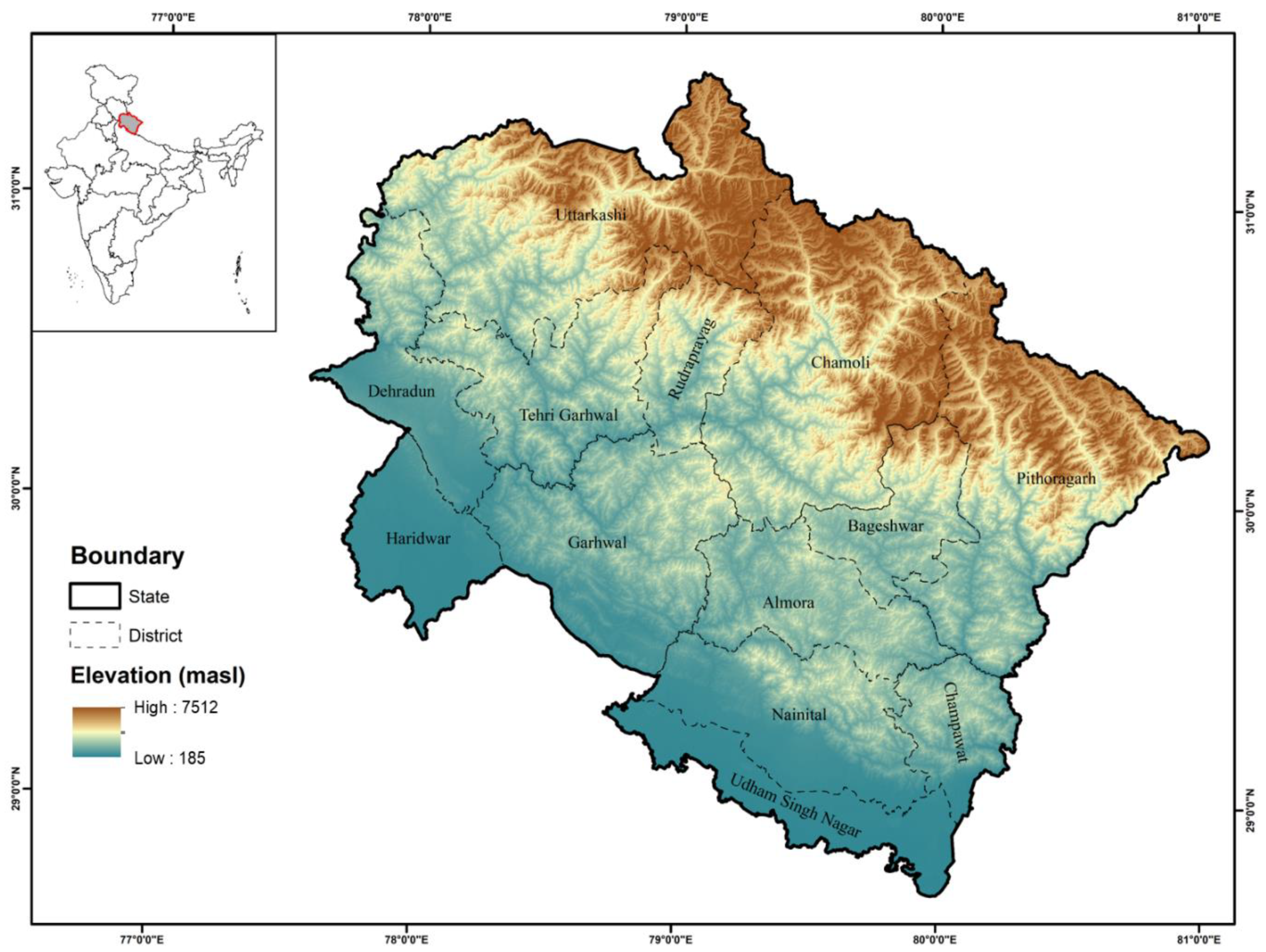
2.1. Study Area

The study area focuses on the Uttarakhand State in the Central Himalaya. Geographically, it is situated between 28°43′24″ to 31°27′50″ North latitude and 77°34′27″ to 81°02′22″ East longitude with an area of 53,485 km2, accounting for 1.62% of the total area of the country (Figure 1). The elevation of the region ranges from 210 to 7817 m. Administratively, the state is divided into 13 districts falling into two administrative divisions, Garhwal (north-west portion) and Kumaon (south-east portion). The entire state is characterized by a wide range of intraregional variations in topography, geology, soil, and climate as well as in socio-economic structure and living standards and development. It has an immense diversity of altitude, climate, natural resources, biodiversity, ethnicity, culture, and farming systems.
The state has a diverse topography and fragile terrain. It can broadly be divided into three physiographic zones, the Greater Himalaya (Himadri), the Lesser Himalaya (Himachal), and the Outer Himalaya (Shivaliks) running parallel to each other from northwest to southeast. The forest cover is 45.44% of its geographical area, with 9.44% very dense forest, 23.94% moderately dense forest, and 12.06% open forest [56]. The major forest types present are Himalayan moist temperate forest (31.64%), subtropical pine forest (29.87%), and tropical moist deciduous (20.29%) forest.
According to the Census of India (2011), the population of Uttarakhand amounts to 10.11 million inhabitants with a population density of 189 individuals per km2. Population distribution in the state is very uneven depending upon the physiography. The state has a sex ratio of 963 females for every 1000 males and a literacy rate of 79.63%. Uttarakhand is predominantly a rural state (69.45% population lives in rural areas) with 16,826 villages, of which 12,699 or 81% have a population of fewer than 500 people. The region is sparsely populated in small settlements with high dependence on rainfed agriculture and adjoining forests. Subsistence agriculture is the main source of livelihood [57,58]. People lack basic facilities such as services and institutions in the region, making them highly dependent on natural resources [59].

2.2. Data Collection

In all, 92 socio-economic variables, such as demography, economy, education, infrastructure, technology, health, etc., and 28 ecological variables addressing climate, geomorphology, biophysical environment, lithology, topography, and land use/cover were collected for the study area based on the earlier mountain-specific literature [35,57,60], discussions with scientific community, and ground observations for a holistic understanding of the considered region (see Table A1 and Table A2 in Appendix A for the complete list of all the variables used). Highly correlated variables were dropped after correlation analysis, resulting in 32 socio-economic and 14 ecological variables (Table 1 and Table 2). For the socio-economic variables, the village was taken as the data collection unit, and the entire database on ecological variables was resampled to 30 m cell size for consistency. Data were collected from different reliable secondary sources namely Census of India (2011), WorldClim database (1970–2000), National Bureau of Soil Survey and Land Use Planning (NBSS&LUP), Forest Survey of India (2015), Biodiversity Characterization program (IIRS/NRSC), National Resource Repository Survey (NRSC), ASTER-GDEM (Advanced Spaceborne Thermal Emission and Reflection Radiometer—Global Digital Elevation Model), MODIS (Moderate Resolution Imaging Spectroradiometer), and a database generated in our laboratory and by others to delineate the boundaries of SESs.

2.3. Data Processing and Analysis

The SES boundary delineation and mapping were carried out with modifications in the methodological approach proposed by Martín-López et al. [1] on a large and heterogeneous area. It was performed in four steps (Figure 2) (a) socio-economic unit identification and characterization, (b) ecological unit identification and characterization, (c) delineation of SES boundaries, and (d) characterization of SES boundaries. R-studio software was used for statistical analysis of the data collected from primary and secondary sources. ArcGIS (ver. 10.1) was used for mapping and spatial analysis.
Multivariate data analysis was performed in R-studio using the “FactoMineR”, “factoextra”, and “ggplot2” packages. Standardization of the variables with different units was done before the analysis, as variables are measured at different scales, which do not contribute equally to the analysis and might end up creating a bias. The Kaiser–Meyer–Olkin (KMO) test [61] was performed to measure sampling adequacy of both datasets of variables (Equation (1)). The KMO test indicates the proportion of variance in variables that might be caused by underlying factors. The KMO test is represented as
K M O j = i j r i j 2 i j r i j 2 + i j u
where rij is the correlation matrix and uij is the partial covariance matrix. The KMO value range between 0 to 1, and if the value is lower than 0.6, then the sampling is not adequate. Bartlett’s test of sphericity [62] was done to test the hypothesis that the correlation matrix is an identity matrix, which indicates that variables are unrelated and, therefore, unsuitable for structure detection. Small values (p < 0.05) of the significance level indicate that data are suitable for principal component analysis (PCA).
For socio-economic units, the villages were considered for clustering since they represent the lowest administrative level. For the delineation of the ecological entities, the state was divided into 250 m grid cells to maintain the data uniformity, and the values for each biophysical variable were calculated for each cell. Subsequently, the values of the variables for socio-economic and ecological units (Table 1 and Table 2) were used in PCA to extract key components for the joint delineation of the SESs. PCA identifies linear independent dimensions by analyzing the similarities between the data points (Equation (2)). PCA is done before clustering for efficiency purposes as algorithms that perform clustering are more efficient for lower-dimensional data. The main objective of PCA is to reduce a dataset (X dataset with m individuals and n variables) with a smaller number of uncorrelated variables (X < n) while retaining as much information as possible. Let X = x i be any k × 1   random vector. We define a k × 1   vector Y = y i , where for each i the i th principal component of X is
y i = j = 1 k β i j x j
For some regression coefficients β i j . Since each y i is a linear combination of the x i , Y is a random vector.
Sequential agglomerative hierarchical cluster analysis (HCA) was applied to the PCs with an eigenvalue greater than 1 (Kaiser criteria), using Euclidean distance and Ward’s method [63] to compute the similarity. It is a stepwise algorithm in which two objects with the least dissimilarity are merged at each step (Equation (3)). The basic concept behind the clustering is Minimize = (Within cluster variance/between cluster variance).
s i m X 1 , X 2 n i = X 1 × X 2 X 1 + X 2 × d i s t M i , M j x k 2
where, X1, X2,…ni are clusters and Mi, Mj,…xk are points. The similarity of clusters X1, X2,…ni is equal to the maximum of the similarity between points Mi, Mj,…xk such that M i belongs to X 1 , and M j belongs to X 2 cluster and n belongs to x k belongs to n i cluster.
The outcome of this analysis is a binary tree, also called a dendrogram, with n−1 nodes characterizing the homogeneous characteristics of a cluster. Usually, the clusters are represented on the y-axis and the similarity or the distance is depicted on the x-axis. The lines that depart from each cluster are linked according to the degree of similarity at which the linkage between clusters happens. The obtained results from separate analyses provide homogeneous socio-economic and ecological units. The socio-economic and ecological units were layered and stored in a fishnet of 250 m grid size. The grid was clustered using the HCA to determine the boundaries of the SESs. For characterization of the mapped SESs, variable contribution in each socio-economic and ecological unit was determined using the variable loadings of the respective PCA. Prominent variables were selected as characteristic features of the SESs. The nomenclature for the SESs was derived using feedback on characteristics from domain experts such as scientists and environmental managers working in the Himalaya through discussions and informal meetings. The feedback helped in the nomenclature and characterization of the SESs.

3. Results

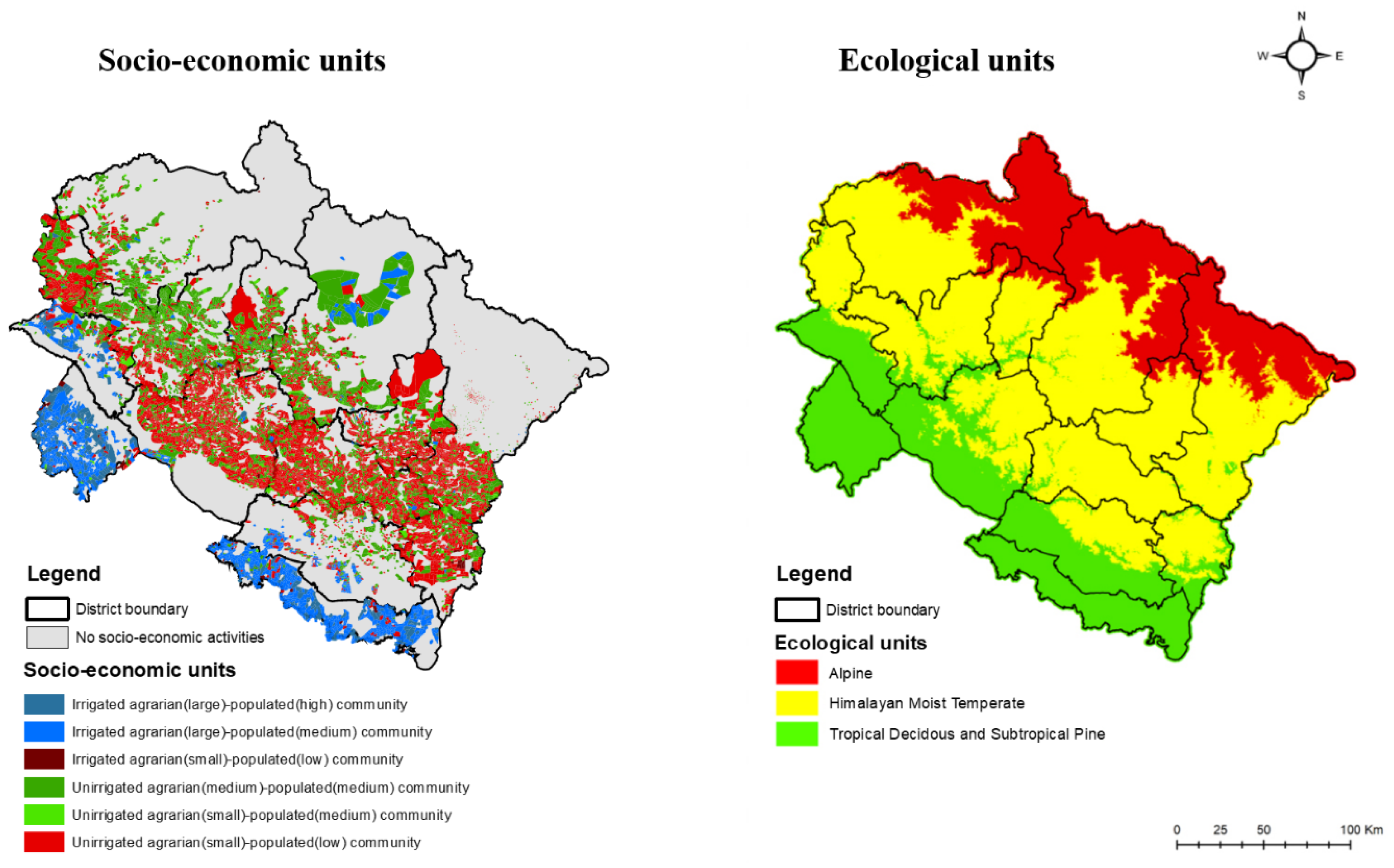
3.1. Socio-Economic Units

The KMO test result gave a value of 0.82, and Bartlett’s test of sphericity showed p < 2.22 × 10⁻¹⁶ for the socio-economic variables. Socio-economic data were accounted for by the first nine PCs with 51.62% of the variability. Performing HCA on these components generated six socio-economic cluster units based on the common grouping of characteristics as illustrated in Figure 3. The distribution of eigenvalues and variability explained by each PCA component is presented in Appendix A (Table A3).
Based on the variable loading for each cluster (Table 3), dominant characterizing features were used for the naming of the units (Table 4). The categorization of these features is presented in Appendix A (Table A4). For instance, Unit 1 (irrigated agrarian (large)–populated (high) community) represents the villages that are large and have well-irrigated land for agriculture. This unit occurs mostly in the plains at the foothills of the Himalaya known as Tarai and Bhabar, covering 1.82 percent of the geographical area. Unit 2 (irrigated agrarian (large)–populated (medium) community) represents the villages that have irrigated land and are modest in size. This unit is mostly present in the lower Himalaya and the valleys of the upper Himalaya covering together 8.82 percent of Uttarakhand. Unit 3 (irrigated agrarian (small)–populated (low) community) represents the villages that have a high population with unirrigated land for agriculture. This unit is distributed in the middle Himalayan region within the elevation range of 1000–2500 m, covering 31.72 percent of the land, thus, being the second-largest unit. Unit 4 (unirrigated agrarian (medium)–populated (medium) community) represents the villages that are small in area and have unirrigated land for agriculture. It is distributed throughout the middle Himalaya covering 4 percent of the area. Unit 5 (unirrigated agrarian (small)–populated (medium) community) represents the small villages, with a high population and unirrigated land for agriculture. It is distributed in the middle and upper Himalaya. It is the dominant unit covering 53.07 percent of the land in the state. Unit 6 (unirrigated agrarian (small)–populated (low) community) represents the villages that have irrigated land with better road connectivity and communication infrastructure. It is the smallest unit covering only 0.51 percent of land and is scattered throughout the Himalaya. In most of the cluster types, agriculture, geographical area, and population were the main epicenters around which the socio-economic strata reforms.

3.2. Ecological Units

For the ecological variables, the KMO test result gave a value of 0.65, and Bartlett’s test of sphericity showed p < 2.22 × 10⁻¹⁶. The distribution of eigenvalues and variability of PCA components is presented in Appendix A (Table A5). In Uttarakhand state, the HCA identified three ecological units illustrated in Figure 3. Based on the variable loadings of cluster units (Table 3), forest types and land use land cover (LULC) classes were identified as the characterizing feature (Table 4). Unit 1 (alpine) represents the alpine-dominated forest group in the state. It covers 20.95 percent of the state area in the upper Himalaya (>2500 m). Unit 2 (Himalayan moist temperate) represents the Himalayan moist temperate forest group and is the largest unit in the state by covering 52.89 percent of the land area. This unit occurs in the middle Himalaya (1000–2500 m). Unit 3 (tropical deciduous and subtropical pine) covers 26.16 percent of the land and occurs in the lower and outer Himalaya (<1000 m).

3.3. Socio-Ecological Systems

The intersection of borders of socio-economic and ecological units determined the SES boundaries. After the delineation, 18 SES classes were generated and identified as shown in Figure 4 (see also Table 5). The key socio-economic and ecological characteristics were selected based on the methodological approach defining SESs in the Himalayan state. The major contributing ecological variable was identified as forest types and the most important socio-economic variable was agricultural practices. These two variables were determinant factors to characterize the generated 18 types of SESs (Table 3). The alpine-forest-based SESs are situated in the upper Himalayan region covering 21.71 percent of the land area, and the majority of this is covered with snow throughout the year. The Himalayan moist temperate forest–based SESs are situated in the middle Himalaya and are the major groups in the state covering 52.29 percent of the state area. Tropical deciduous and subtropical pine–based SESs are situated in the foothills and lower Himalaya covering 26 percent of the land area.
The Himalayan moist temperate/unirrigated agrarian (small)–populated (low) community (B6) within the middle Himalaya is the major socio-ecological system with 13.38% cover in the state. This system has small villages with low farm holdings in a temperate climate. The other major system is the Himalayan moist temperate/unirrigated agrarian (medium)–populated (medium) community (B4) covering 11.55% in the middle Himalaya. In this system, the villages have a moderate population linked with a temperate climate. These two systems with temperate climate are located in the middle Himalaya. The villages are sparsely populated and have mostly unirrigated agriculture, making the communities highly dependent on forest resources due to the geographical setting of the region. In the lower Himalaya, the major SESs are the tropical deciduous and subtropical pine/irrigated agrarian (large)–populated (medium) community (C2) with 4.51% and the tropical deciduous and subtropical pine/unirrigated agrarian (small)–populated (low) community (C6) with 3.71%.
The spatial mapping shows two pertinent aspects of the Himalaya, the ecosystem and the society. Our mapping highlights the interactions and linkages between the ecological subsystems and social systems (Figure 5). The alpine ecological unit is dominated by social systems with large-to-medium irrigated land and medium population density (A2, A4, and A6). These are more in the high altitudes of the mountain systems. The Himalayan moist temperate forest shows a much wider range of linkages across the social units of the region. These are dominated by villages with low-to-medium population with unirrigated agrarian practices (B1, B2, B3, B4, B5, and B6). However, it also supports other social units. These ecological systems range from low-to-medium altitude with select pockets in high-altitude regions. The tropical deciduous and subtropical pine forests also share a wider linkage across all the social units of the Central Himalaya. These exhibit a stronger linkage with irrigated large agrarian–medium population communities (C1, C2, C3, C4, C5, and C6). Unlike the Himalayan moist temperate forest, these do not have a wider distribution and are restricted much to lower altitudes and a few ranges of middle altitude.

4. Discussion

Identification and spatial mapping of SESs at the regional level is demanding since administrative borders often do not coincide with natural variables that determine how nature is managed by people. Therefore, an interdisciplinary approach is required that supports integrating a wide range of variables considering social and ecological interactions. Most of the earlier studies [1,5,10,11,22] have mapped these for a smaller geographical area (e.g., regional, municipality, national park) or with a focus on particular system types. Martín-López et al. [1] identified SESs at a local level to understand the interaction at the local level, which can be useful for meta-analysis of the individual SESs. In addition to the understanding of the cross-disciplinary approaches, the geospatial tools and data integration capability have enhanced opportunities to analyze potential and complex relationships and interactions between social and ecological systems [64,65]. Researchers have leveraged such capabilities to identify and map different ecological units [66,67,68]. The identification and spatial mapping of SESs in the Central Himalaya presented in this study is one of the first attempts to develop an indicator-based model. It extends previous efforts of mapping SESs [1,11,22], in that it takes a broader range of both social and ecological variables into account. Such an attempt has multiple advantages and a few limitations, which can assist researchers to replicate, reproduce, and enhance it over time to identify changes in social-ecological systems, essential to policy planning [22].
These intricate linkages between the ecological and social systems indicate the distinct vulnerability and adaptive capacities of the communities to climate change. The relationships also explain the dependence of the socio-economic units on the ecological units, indicating higher dependence on forests. For example, Himalayan moist temperate forests are known for the resource utilization structures, processes, and patterns in the region, and thus these are highly associated with the forests, farmland, and livestock [69,70]. Similarly, the dependence is higher on the tropical deciduous and subtropical pine forest and the least on the alpine ecological units. Such relationships also indicate the services and support rendered by these ecological units to the socio-economic units in the Central Himalaya. These provide multiple ecosystem services including much of the supporting and regulating services for such communities, e.g., biomass production, soil formation and retention, nutrient cycling, provisioning of habitat, and regulation of climate and water [71].

4.1. Advancement in Methods

The presented methodological framework combines the multivariate analysis of both biophysical and socio-economic variables using GIS to identify and characterize the SESs [1]. The study generated SESs at the regional level with characteristics features though the SESs are nested at multiple spatial levels [3]. The modified methodology has similar limitations that have been noted by others in their studies [1,22,72]. Few of the variables’ data were not available at the local level in the study, so that they had to be downscaled, and this increased the data-borne uncertainty of the mapping exercise [73]. Our analysis suggests that there is a need to carefully consider scale to generate SES units. Analyses at multiple spatial scales will reveal different patterns of complexity and dynamics, thus, limiting the recognition of the complex dynamics of SESs. Our approach is limited by the availability of data. For example, factors responsible for governance are not included in the approach [6]. In order to interpret large datasets, methods are required to drastically reduce their dimensionality in an interpretable way, such that most of the information in the data is preserved. It gives the best possible representation of a p-dimensional dataset in q dimensions (q < p) in the sense of maximizing variance in q dimensions. A disadvantage is, however, that the new variables that it defines are usually linear functions of all p original variables, and there is a trade-off between interpretability and variance [74]. In this study, since the original random variables are non-Gaussian distributed, their linear combinations were non-Gaussian distributed, and uncorrelated principal components were independent. The removal of outliers does create a normal distribution in some of the variables, but for some variables, outliers are informative about the subject area and data collection process, which was essential in the study to understand the spatial complexity.
The framework helps in replacing the general administrative boundary criteria used in adaptation and landscape planning using a socio-ecological approach. From a social scientific point of view, the boundaries on a map do not correspond with the association of the physical and social world [75]. The perceived boundaries of SESs can vary among actors considering their landscape-scale usage patterns [1]. Cross-scale modeling concepts have emerged in landscape ecology as a way to better capture complex system characteristics to support science and practitioner interactions [76]. These abstractions of the real-world address different types of governance, how resources are influenced, and how human action or behavior affects the ecosystem’s performance [77].

4.2. Relevance and Applicability of the Method

This study provides a robust methodology to delineate and characterize SESs, which could be adopted in the entire Himalayan arc and in other mountain ecosystems of the world. Mapped SESs can provide a basic template for studies in mountain ecosystems related to climate change impacts, vulnerability assessment, adaptation planning, risk and hazards assessment, the resilience of communities to multiple stressors, natural resource management, and policy- and decision-making. Characterizing multilevel interactions from local communities to national decision-makers encourages robust policy-making to ensure sustainable resource management [78]. Combining practitioners’ knowledge with socio-economic and environmental changes in modeling platforms acts as a vehicle toward proactive spatial assessment and planning. Pivotal for policy-making is a better recognition of cross-disciplinary models to ensure information and communication flows for developing landscape as well as adaptation planning strategies [79]. The mapped SESs help in recognizing local needs and gaps in existing policies and institutional arrangements. Taking SES as a coupled system will help policymakers to look at two fronts as a single unit. Beyond these practicum usages, the study fills a wide gap in SES approaches for vulnerability assessment in mountain ecosystems as it considers the differences and associations of socio-economic and ecological system characteristics and acts as a tool for policy implementation to reduce vulnerability [80]. This would pave the pathways for future academic and research-based studies. Understanding the SESs can help in explaining the natural resource usage pattern by the communities of socio-economic units and major ecosystem services. Homogenous ecological units have similar kinds of services and usage patterns. This helps in analyzing and modeling SES interactions to better understand feedback, non-linearity, and the future dynamics of drivers across multiple scales [81].

4.3. Outlook

India is classified into 15 agroclimatic zones by the National Bureau of Soil Survey and Land Use Planning (NBSS&LUP). These zones are classified based on climatic factors, soil properties, physiographic settings, geological formation, climate, cropping patterns, and development of irrigation and mineral resources. Uttarakhand state is classified as a Western Himalayan agroclimatic zone. It is further divided into two subclasses, namely Hill (AZ26) and Bhabar and Tarai (AZ27). Our approach identified seven different types of SESs in the Bhabar and Tarai (AZ27) zone and eleven types of SESs in the Hill (AZ26) zone with distinct features providing more details for planning. Agroclimatic zonation and other similar approaches such as biome [66] and bio-geographical zone [82] mapping mainly address ecological settings but do not take into account the association of communities and institutions. To our knowledge, this is the first time that census data on resource use have been used to identify and map SESs in the Himalayan landscape. Therefore, the developed database and method can be used as a tool for locally adapted actors and institutions for efficient planning and management. The studied cases of Uttarakhand state showed that there is a need for locally suitable adaptation planning and management to avoid a one size fits all strategy [17,83] in social and ecological aspects. The SESs provide variation and specific features pertinent to the interlinked network of resource systems and actors [6].
A study by Dressel et al. [22] used PCA on multiple socio-ecological variables to understand the socio-ecological context of natural resource management. Martín-López et al. [1] identified SES boundaries to explain their importance in landscape planning for managing ecosystem services. Our approach used a similar principle but focused on characterizing a larger geographical entity in mountain systems to provide SESs boundaries and improve the understanding of the characteristics that define the SESs.

5. Conclusions

The study has demonstrated an approach to identify and spatially map socio-ecological systems in the Central Himalaya. It developed an indicator-based model on an understanding of the intricate relationship between social systems and ecological systems and by explaining the characteristic features over a large heterogeneous area. This is the first time that census data on resource and biophysical variables on ecological distribution area were used to identify and map SESs in the Himalayan region. The approach differs from earlier attempts at mapping ecological units and linking with social data to describe the socio-ecological system. The SESs mapping will help in improving the currently practiced mapping approach in the Himalayan region for socio-economic and ecological planning and management. The approach presented here may be a practical tool that can be replicated and reproduced across mountain ecosystems. The subsequent understandings will, therefore, support the preparation of adaptation plans to cope with the impacts of climate change in the Himalayan region and sustainable natural resource management. Our approach is a beneficial tool to analyze and represent the multidimensional systems of mountainous regions to help decision- and policymakers develop site-specific policies. The future challenges in SES research involve the understanding of dynamics at multiple scales and the development of credible measures of evaluation, corporate governance, and promotion of adaptation. To understand the complexity of the SESs, a further meta-analysis by integrating participatory methods for each system is necessary. Overall, a rigorous and in-depth approach is necessary to combat these situations.

Author Contributions

Conceptualization, P.K.J. and P.K.; methodology, P.K. and P.K.J.; software, P.K. and C.F.; validation, P.K. and P.K.J.; formal analysis, P.K.; investigation, P.K.J. and P.K.; resources, P.K.J. and C.F.; data curation, P.K.; writing—original draft preparation, P.K.; writing—review and editing, P.K., P.K.J., and C.F.; visualization, P.K.J. and P.K.; supervision, P.K.J. and C.F.; project administration, P.K.J.; funding acquisition, C.F. All authors have read and agreed to the published version of the manuscript.

Funding

P.K. would like to acknowledge a UGC-JRF scholarship by the University Grants Commission, Ministry of Human Resource Development, Government of India; and a DAAD scholarship, Federal government of Germany, for funding his doctoral research.

Data Availability Statement

The data presented in this study are available in this article.

Acknowledgments

The authors would like to acknowledge the Institute for Geosciences and Geography at Martin Luther University, Halle, Germany, for their support in providing a high-performance computing facility for data analysis. Authors are also thankful to the reviewers and editorial board for comments and advice to improve the quality of manuscript.

Conflicts of Interest

The authors declare no conflict of interest. The funders had no role in the design of the study; in the collection, analyses, or interpretation of data; in the writing of the manuscript; or in the decision to publish the results.

Appendix A

Table A1. List of total variables used to form ecological units.
 Type Variable Name Code Data Source
 Climatic Climatic Annual Mean Temperature BIO 1 WorldClim
 Mean Diurnal Range BIO 2 WorldClim
 Isothermality (BIO 2/BIO 7) (×100) BIO 3 WorldClim
 Temperature Seasonality (Standard Deviation × 100) BIO 4 WorldClim
 Max. Temperature of Warmest Month BIO 5 WorldClim
 Min. Temperature of Coldest Month BIO 6 WorldClim
 Temperature Annual Range (BIO 5-BIO 6) BIO 7 WorldClim
 Mean Temperature of Wettest Quarter BIO 8 WorldClim
 Mean Temperature of Driest Quarter BIO 9 WorldClim
 Mean Temperature of Warmest Quarter BIO 10 WorldClim
 Mean Temperature of Coldest Quarter BIO 11 WorldClim
 Annual Precipitation BIO 12 WorldClim
 Precipitation of Wettest Month BIO 13 WorldClim
 Precipitation of Driest Month BIO 14 WorldClim
 Precipitation Seasonality (Coefficient of Variation) BIO 15 WorldClim
 Precipitation of Wettest Quarter BIO 16 WorldClim
 Precipitation of Driest Quarter BIO 17 WorldClim
 Precipitation of Warmest Quarter BIO 18 WorldClim
 Precipitation of Coldest Quarter BIO 19 WorldClim
 Geomorphologic Elevation Elv ASTER-GDEM
 Aspect Asp ASTER-GDEM
 Slope Slp ASTER-GDEM
 Pedologic Soil type Soil National Bureau of Soil
Survey and Land Use Planning
 Land use/Land cover LULC LULC National Remote Sensing Center
 Forest Cover Forest Types Frst Forest Survey of India
 Biophysical Normalized Difference Vegetation Index NDVI MODIS
 Enhanced Vegetation Index EVI MODIS
 Normalized Difference Water Index NDWI MODIS
Table A2. List of total variables used to form socio-economic units (source: Census of India, 2011).
 TypeVariables
 Demographics Total Geographical Area (in Hectares) Total Households  Total Population of Village
 Primary Education (Numbers) Govt. Preprimary School (Nursery/LKG/UKG)  Private Preprimary School (Nursery/LKG/UKG)  Govt. Primary School  Private Primary School
 Secondary School (Numbers) Govt. Middle School Private Middle School  Govt. Secondary School  Private Secondary School
 Govt. Senior Secondary School  Private Senior Secondary School
 Higher Education (Numbers) Govt. Arts and Science Degree College  Private Arts and Science Degree College  Govt. Engineering College  Private Engineering College
 Govt. Medical College  Private Medical College
 Healthcare (Numbers) Community Health Center  Primary Health Center  Primary Health Subcenter  Maternity And Child Welfare Center  Family Welfare Center
 Hospital—Allopathic  Hospital—Alternative Medicine  Dispensary  Mobile Health Clinic
 Toilet Toilet Complex (including Bath)
 Tap Water  Tap Water—Treated Tap Water—Untreated
 Well Covered Well Uncovered Well
 Hand Pump/Tube Wells Hand Pump Tube Wells/Borehole
 River/Canal/Tank/Pond/Lake River/Canal Tank/Pond/Lake  Spring
 Post Office  Post Office Sub-Post Office Post and Telegraph Office
 Communication  Public Call Office/Mobile (PCO)  Mobile Phone Coverage Internet Cafes/Common Service Center (CSC) Telephone
 Transportation  Public Bus Service  Private Bus Service Railway Station Auto/Modified Autos Taxi
 Road Connectivity  Black Topped (pakka) Road Gravel (kuchha) Roads Water-Bound Macadam
 All-Weather Road State Highway National Highway
 Bank Services ATM Commercial Bank Cooperative Bank
 Credit Societies Agricultural Credit Societies Self-Help Group (SHG)
 Market Mandis/Regular Market  Weekly Haat Public Distribution System (PDS) Shop
 Govt. Health Program Nutritional Centers—Anganwadi Center ASHA
 Waste Disposal Waste Disposal System after House-to-House Collection  Bio-gas or Recycling of Waste for Production Use
 Media Community Center with/without TV Sports Club/Recreation Center Cinema/Video Hall
 Information Public Library Public Reading Room Daily Newspaper Supply Assembly Polling Station
 Agriculture Infrastructure Agriculture Equipment Tractors Carts Driven by Animals
 Electricity Power Supply for Domestic Use Power Supply for Agriculture Use Power Supply for Commercial Use
Agricultural Land Culturable Waste Land Area (in Hectares) Fallows Land other than Current Fallows Area (in Hectares) Current Fallows Area (in Hectares)
 Net Area Sown (in Hectares) Total Unirrigated Land Area (in Hectares) Area Irrigated by Source (in Hectares)
 Land Forest Area (in Hectares) Area under Non-Agricultural Uses (in Hectares) Barren and Un-cultivable Land Area (in Hectares)
 Permanent Pastures and Other Grazing Land Area (in Hectares) Land under Miscellaneous Tree Crops, etc., Area (in Hectares)
Table A3. Distribution of eigenvalues and variability by PCA components for socio-economic units.
ComponentEigenvaluePercentage of VarianceCumulative Percentage of Variance
15.020518216.1952216.19522
22.48336448.01085324.20607
31.55943665.03044129.23651
41.44011374.64552833.88204
51.19210833.84551137.72755
61.14921323.70713941.43469
71.10198713.55479744.98949
81.05161043.39229248.38178
91.00668723.24737851.62916
100.98936153.19148954.82065
110.97037793.13025157.9509
120.95576073.08309961.034
130.90768262.92800863.96201
140.88882572.8671866.82919
150.87386072.81890669.64809
160.86037752.77541172.4235
170.85367642.75379575.1773
180.80783022.60590477.7832
190.78679552.5380580.32125
200.74926322.41697882.73823
210.6993982.25612384.99435
220.68634012.21487.20835
230.63322952.04267689.25103
240.58553291.88881691.13984
250.5565951.79546892.93531
260.52094811.68047894.61579
270.45850951.47906396.09485
280.42053021.35654997.4514
290.40581921.30909498.7605
300.24511170.79068399.55118
310.13913450.448821100
Table A4. Categorization of the socio-economic units with their mean households and area per village.
Socio-Economic UnitNumber of VillagesMean Area per Village (in Hectares)Large/Medium/SmallMean Households per VillageHigh/Medium/Low
Irrigated agrarian (large)–populated (high) community278452.3L646H
Irrigated agrarian (large)–populated (medium) community1357165.19L188M
Irrigated agrarian (small)–populated (low) community7885.23S13L
Unirrigated agrarian (medium)–populated (medium) community4849104.79M74M
Unirrigated agrarian (small)–populated (medium) community61179.6S51M
Unirrigated agrarian (small)–populated (low) community811257.35S27L
Table A5. Distribution of eigenvalues and variability by PCA components for ecological units.
ComponentEigenvaluePercentage of VarianceCumulative Percentage of Variance
14.843334.59534.595
23.3768724.120558.7155
31.5936711.383470.0989
41.002647.1617477.2607
50.838425.988783.2494
60.74595.3278488.5772
70.572574.0897892.667
80.473213.3800896.0471
90.324442.3174198.3645
100.131740.9409899.3054
110.059240.4231699.7286
120.028810.2057999.9344
130.007580.0541599.9886
140.00160.01145100
Figure A1. Variable contribution in the socio-economic unit clustering from units (16); and in the ecological unit clustering from units (AC).
Sustainability 13 07525 g0a1

References

  1. Martín-López, B.L.; Palomo, I.; García-Llorente, M.; Iniesta-Arandia, I.; Castro, A.J.; del Amo, D.G.; Gómez-Baggethun, E.; Montes, C. Delineating boundaries of social-ecological systems for landscape planning: A comprehensive spatial approach. Land Use Policy 2017, 66, 90–104. [Google Scholar] [CrossRef]
  2. Gallopín, G.C.; Gutman, P. and Maletta, H. Global impoverishment, sustainable development and the environment: A conceptual approach. Int. Soc. Sci. J. 1989, 121, 375–397. [Google Scholar]
  3. Berkes, F.; Folke, C. Linking Social and Ecological Systems: Management Practices and Social Mechanisms for Building Resilience; Cambridge University Press: Cambridge, UK, 1998. [Google Scholar]
  4. Turner, B.L.; Matson, P.A.; McCarthy, J.J.; Corell, R.W.; Christensen, L.; Eckley, N.; Hovelsrud-Broda, G.K.; Kasperson, J.X.; Kasperson, R.E.; Luers, A.; et al. Illustrating the coupled human–environment system for vulnerability analysis: Three case studies. Proc. Natl. Acad. Sci. USA 2003, 100, 8080–8085. [Google Scholar] [CrossRef] [Green Version]
  5. Liu, J.; Dietz, T.; Carpenter, S.R.; Alberti, M.; Folke, C.; Moran, E.; Pell, A.N.; Deadman, P.; Kratz, T.; Lubchenco, J.; et al. Complexity of Coupled Human and Natural Systems. Science 2007, 317, 1513–1516. [Google Scholar] [CrossRef] [Green Version]
  6. Ostrom, E. A General Framework for Analyzing Sustainability of Social-Ecological Systems. Science 2009, 325, 419–422. [Google Scholar] [CrossRef]
  7. Turner, B.; Kasperson, R.E.; Meyer, W.B.; Dow, K.M.; Golding, D.; Kasperson, J.X.; Mitchell, R.C.; Ratick, S.J. Two types of global environmental change: Definitional and spatial-scale issues in their human dimensions. Glob. Environ. Chang. 1990, 1, 14–22. [Google Scholar] [CrossRef]
  8. Vitousek, P.M.; Mooney, H.A.; Lubchenco, J.; Melillo, J.M. Human Domination of Earth’s Ecosystems. Science 1997, 277, 494–499. [Google Scholar] [CrossRef] [Green Version]
  9. Kates, R.W.; Clark, W.C. Our Common Journey: A Transition toward Sustainability; National Research Council: Washington, DC, USA, 1999. [Google Scholar]
  10. Fairweather, J. Farmer models of socio-ecologic systems: Application of causal mapping across multiple locations. Ecol. Model. 2010, 221, 555–562. [Google Scholar] [CrossRef]
  11. Abson, D.J.; Dougill, A.J.; Stringer, L. Using Principal Component Analysis for information-rich socio-ecological vulnerability mapping in Southern Africa. Appl. Geogr. 2012, 35, 515–524. [Google Scholar] [CrossRef]
  12. Gupta, K.A.; Negi, M.; Nandy, S.; Kumar, M.; Singh, V.; Donatella, V.; Petrosillo, I.; Pandey, R. Mapping socio-environmental vulnerability to climate change in different altitude zones in the Indian Himalayas. Ecol. Indic. 2019, 109, 105787. [Google Scholar] [CrossRef]
  13. Schneider, S.H.; Londer, R. The Coevolution of Climate and Life; Sierra Club Books: San Francisco, CA, USA, 1984. [Google Scholar]
  14. Berkes, F.; Colding, J.; Folke, C. Navigating Social-Ecological Systems: Building Resilience for Complexity and Change; Cambridge University Press: Cambridge, UK, 2003; Volume 9. [Google Scholar]
  15. Rosa, E.A.; Dietz, T. Climate Change and Society: Speculation, Construction and Scientific Investigation. Int. Sociol. 1998, 13, 421–455. [Google Scholar] [CrossRef]
  16. Folke, C.; Hahn, T.; Olsson, P.; Norberg, J. Adaptive governance of social-ecological systems. Annu. Rev. Environ. Resour. 2005, 30, 441–473. [Google Scholar] [CrossRef] [Green Version]
  17. Folke, C.; Pritchard, J.L.; Berkes, F.; Colding, J.; Svedin, U. The Problem of Fit between Ecosystems and Institutions: Ten Years Later. Ecol. Soc. 2007, 12. [Google Scholar] [CrossRef] [Green Version]
  18. Glaser, M.; Krause, G.; Ratter, B.; Welp, M. Human/Nature Interaction in the Anthropocene Potential of Social-Ecological Systems Analysis. GAIA Ecol. Perspect. Sci. Soc. 2008, 17, 77–80. [Google Scholar] [CrossRef]
  19. Gunderson, L.H.; Holling, C.S. (Eds.) Panarchy: Uderstanding Transformations in Human and Natural Systems; Island Press: Washington, DC, USA, 1998. [Google Scholar]
  20. Levin, S.; Xepapadeas, T.; Crépin, A.-S.; Norberg, J.; de Zeeuw, A.; Folke, C.; Hughes, T.; Arrow, K.; Barrett, S.; Daily, G.; et al. Social-ecological systems as complex adaptive systems: Modeling and policy implications. Environ. Dev. Econ. 2012, 18, 111–132. [Google Scholar] [CrossRef] [Green Version]
  21. Preiser, R.; Biggs, R.; de Vos, A.; Folke, C. Social-ecological systems as complex adaptive systems: Organizing principles for advancing research methods and approaches. Ecol. Soc. 2018, 23, 46. [Google Scholar] [CrossRef] [Green Version]
  22. Dressel, S.; Ericsson, G.; Sandström, C. Mapping social-ecological systems to understand the challenges underlying wildlife management. Environ. Sci. Policy 2018, 84, 105–112. [Google Scholar] [CrossRef]
  23. Dechazal, J.; Quétier, F.; Lavorel, S.; VanDoorn, A. Including multiple differing stakeholder values into vulnerability assessments of socio-ecological systems. Glob. Environ. Chang. 2008, 18, 508–520. [Google Scholar] [CrossRef]
  24. McClanahan, T.R.; Castilla, J.C.; White, A.T.; Defeo, O. Healing small-scale fisheries by facilitating complex socio-ecological systems. Rev. Fish Biol. Fish. 2009, 19, 33–47. [Google Scholar] [CrossRef]
  25. Castellarini, F.; Siebe, C.; Lazos, E.; de la Tejera, B.; Cotler, H.; Pacheco, C.; Boege, E.; Moreno, A.R.; Saldívar, A.; Larrazabal, A.; et al. A social-ecological spatial framework for policy design towards sustainability: Mexico as a study case. Investig. Ambient. Cienc. Política Pública 2014, 6, 45–59. [Google Scholar]
  26. Auty, R.M. Resource Abundance and Economic Development; Oxford University Press: Oxford, UK, 2001. [Google Scholar]
  27. Omernik, J.M. Ecoregions of the Conterminous United States. Ann. Assoc. Am. Geogr. 1987, 77, 118–125. [Google Scholar] [CrossRef]
  28. Olson, D.M.; Dinerstein, E. The Global 200: A Representation Approach to Conserving the Earth’s Most Biologically Valuable Ecoregions. Conserv. Biol. 1998, 12, 502–515. [Google Scholar] [CrossRef] [Green Version]
  29. Cockburn, J.; Cundill, G.; Shackleton, S.; Rouget, M. Towards Place-Based Research to Support Social–Ecological Stewardship. Sustainability 2018, 10, 1434. [Google Scholar] [CrossRef] [Green Version]
  30. Barreteau, O.; Giband, D.; Schoon, M.; Cerceau, J.; DeClerck, F.; Ghiotti, S.; James, T.; Masterson, V.A.; Mathevet, R.; Rode, S.; et al. Bringing together social-ecological system and territoire concepts to explore nature-society dynamics. Ecol. Soc. 2016, 21, 42. [Google Scholar] [CrossRef] [Green Version]
  31. Hamann, M.; Biggs, R.; Reyers, B. Mapping social-ecological systems: Identifying ‘green-loop’ and ‘red-loop’ dynamics based on characteristic bundles of ecosystem service use. Glob. Environ. Chang. 2015, 34, 218–226. [Google Scholar] [CrossRef]
  32. Wymann, S.; Ott, C.; Andreas, K.; Stillhardt, B. Will International Pursuit of the Millennium Development Goals Alleviate Poverty in Mountains? Mt. Res. Dev. 2006, 26, 4–8. [Google Scholar]
  33. Ning, W.; Rawat, G.S.; Joshi, S.; Ismail, M.; Sharma, E. High-Altitude Rangelands and Their Interfaces in the Hindu Kush Himalayas; ICIMOD: Kathmandu, Nepal, 2013. [Google Scholar]
  34. Singh, S.P.; Thadani, R. Complexities and Controversies in Himalayan Research: A Call for Collaboration and Rigor for Better Data. Mt. Res. Dev. 2015, 35, 401–409. [Google Scholar] [CrossRef]
  35. Gerlitz, J.Y.; Macchi, M.; Brooks, N.; Pandey, R.; Banerjee, S.; Jha, S.K. The Multidimensional Livelihood Vulnerabil-ity Index—An instrument to measure livelihood vulnerability to change in the Hindu Kush Himalayas. Clim. Dev. 2017, 9, 124–140. [Google Scholar] [CrossRef]
  36. Kohler, T.; Maselli, D. (Eds.) Mountains and Climate Change—From Understanding to Action; Geographica Bernensia with the support of the Swiss Agency for Development and Cooperation (SDC), and an international team of contributors: Bern, Switzerland, 2009.
  37. Egan, P.; Price, M. Mountain Ecosystem Services and Climate Change: A Global Overview of Potential Threats and Strategies for Adaptation; UNESCO: Paris, France, 2017. [Google Scholar]
  38. Beniston, M. Climatic Change in Mountain Regions: A Review of Possible Impacts. Clim. Chang. 2003, 59, 5–31. [Google Scholar] [CrossRef]
  39. Binder, C.R.; Hinkel, J.; Bots, P.W.G.; Pahl-Wostl, C. Comparison of Frameworks for Analyzing Social-ecological Systems. Ecol. Soc. 2013, 18, 26. [Google Scholar] [CrossRef] [Green Version]
  40. Rissman, A.R.; Gillon, S. Where Are Ecology and Biodiversity in Social–Ecological Systems Research? A Review of Research Methods and Applied Recommendations. Conserv. Lett. 2016, 10, 86–93. [Google Scholar] [CrossRef]
  41. ICIMOD. Mountain, Green Economy for Sustainable Development: A Concept Paper for Rio+20 and Beyond. In International Conference on Green Economy and Sustainable Mountain Development Opportunities and Challenges in View of Rio+20; ICIMOD: Kathmandu, Nepal, 2011. [Google Scholar]
  42. Gerlitz, J.-Y.; Hunzai, K.; Hoermann, B. Mountain poverty in the Hindu-Kush Himalayas. Can. J. Dev. Stud. 2012, 33, 250–265. [Google Scholar] [CrossRef]
  43. Pathak, D.; Gajurel, A.P.; Mool, P.K. Climate Change Impacts on Hazards in the Eastern Himalayas; ICIMOD: Kathmandu, Nepal, 2010. [Google Scholar]
  44. ICIMOD. The Changing Himalayas: Impact of Climate Change on Water Resources and Livelihoods in the Greater Himalayas; ICIMOD: Kathmandu, Nepal, 2009. [Google Scholar]
  45. Ray, M.; Doshi, N.; Alag, N.; Sreedhar, R. Climate Vulnerability in North Western Himalayas; Indian Network on Ethics and Climate Change (INECC): Visakhapatnam, India, 2011. [Google Scholar]
  46. UAPCC. Uttarakhand Action Plan on Climate Change; Government of Uttarakhand: Dehradun, India, 2014.
  47. Xu, J.; Grumbine, R.E.; Shrestha, A.; Eriksson, M.; Yang, X.; Wang, Y.U.N.; Wikes, A. The melting Himalayas: Cascading effects of climate change on water, biodiversity, and livelihoods. Conserv. Biol. 2009, 23, 520–530. [Google Scholar] [CrossRef]
  48. Negi, G.C.S.; Samal, P.K.; Kuniyal, J.C.; Kothyari, B.P.; Sharma, R.K.; Dhyani, P.P. Impact of climate change on the western Himalayan mountain ecosystems: An overview. Trop. Ecol. 2012, 53, 345–356. [Google Scholar]
  49. Madhura, R.K.; Krishnan, R.; Revadekar, J.; Mujumdar, M.; Goswami, B.N. Changes in western disturbances over the Western Himalayas in a warming environment. Clim. Dyn. 2015, 44, 1157–1168. [Google Scholar] [CrossRef]
  50. Jing, F.; Leduc, B. Potential Threats from Climate Change to Human Wellbeing in the Eastern Himalayan Region; Climate Change Impact and Vulnerability in the Eastern Himalayas: Technical Report 6; ICIMOD: Kathmandu, Nepal, 2010. [Google Scholar]
  51. Sarkar, S.; Kanungo, D.P.; Sharma, S. Landslide hazard assessment in the upper Alaknanda valley of Indian Himalayas. Geomat. Nat. Hazards Risk 2015, 6, 308–325. [Google Scholar] [CrossRef] [Green Version]
  52. Chaudhary, P.; Bawa, K.S. Local perceptions of climate change validated by scientific evidence in the Himalayas. Biol. Lett. 2011, 7, 767–770. [Google Scholar] [CrossRef] [Green Version]
  53. Tiwari, P.C.; Joshi, B. Environmental Changes and their Impact on Rural Water, Food, Livelihood and Health Security in Kumaon Himalayas. J. Urban Reg. Stud. Contemp. India 2014, 1, 1–12. [Google Scholar]
  54. INCCA. 2010. Climate Change and India: A 4 × 4 Assessment. A Sectoral and Regional Analysis for 2030S; Ministry of Environment, Forests and Climate Change, Government of India: New Delhi, India, 2010.
  55. Olsson, L.; Jerneck, A. Social fields and natural systems: Integrating knowledge about society and nature. Ecol. Soc. 2018, 23. [Google Scholar] [CrossRef] [Green Version]
  56. ISFR. India State of Forest Report; Forest Survey of India, Ministry of Environment, Forests and Climate Change: Dehradun, India, 2019.
  57. Barua, A.; Katyaini, S.; Mili, B.; Gooch, P. Climate change and poverty: Building resilience of rural mountain com-munities in South Sikkim, Eastern Himalaya, India. Reg. Environ. Chang. 2014, 14, 267–280. [Google Scholar] [CrossRef]
  58. Pandey, R.; Bardsley, D.K. Social-ecological vulnerability to climate change in the Nepali Himalaya. Appl. Geogr. 2015, 64, 74–86. [Google Scholar] [CrossRef] [Green Version]
  59. Hunzai, K.; Gerlitz, J.-Y.; Hoermann, B. Understanding Mountain Poverty in the Hindu Kush-Himalayas—Regional Report for Afghanistan, Bangladesh, Bhutan, China, India, Myanmar, Nepal, and Pakistan; International Centre for Integrated Mountain Development (ICIMOD): Kathmandu, Nepal, 2011. [Google Scholar]
  60. Chakraborty, A.; Joshi, P.; Sachdeva, K. Predicting distribution of major forest tree species to potential impacts of climate change in the central Himalayan region. Ecol. Eng. 2016, 97, 593–609. [Google Scholar] [CrossRef]
  61. Kaiser, H.F.; Rice, J. Little Jiffy, Mark IV. Educ. Psychol. Meas. 1974, 34, 111–117. [Google Scholar] [CrossRef]
  62. Bartlett, M.S. The effect of standardization on a Chi-square approximation in factor analysis. Biometrika 1951, 38, 337–344. [Google Scholar]
  63. Ward, J.H., Jr. Hierarchical Grouping to Optimize an Objective Function. J. Am. Stat. Assoc. 1963, 58, 236–244. [Google Scholar] [CrossRef]
  64. Bateman, I.J.; Jones, A.P.; Lovett, A.A.; Lake, I.; Day, B.H. Applying Geographical Information Systems (GIS) to Environmental and Resource Economics. Environ. Resour. Econ. 2002, 22, 219–269. [Google Scholar] [CrossRef]
  65. Maes, J.; Egoh, B.; Willemen, L.; Liquete, C.; Vihervaara, P.; Schägner, J.P.; Grizzetti, B.; Drakou, E.; La Notte, A.; Zulian, G.; et al. Mapping ecosystem services for policy support and decision making in the European Union. Ecosyst. Serv. 2012, 1, 31–39. [Google Scholar] [CrossRef]
  66. Roy, P.; Joshi, P.K.; Shavindar, S.; Agarwal, S.; Drswapanil, Y.; Jeganathan, C. Biome mapping in India using vegetation type map derived using temporal satellite data and environmental parameters. Ecol. Model. 2006, 197, 148–158. [Google Scholar] [CrossRef]
  67. Ellis, R.; Ramankutty, N. Putting people in the map: Anthropogenic biomes of the world. Front. Ecol. 2008, 6, 439–447. [Google Scholar] [CrossRef] [Green Version]
  68. Ellis, E.C.; Klein Goldewijk, K.; Siebert, S.; Lightman, D.; Ramankutty, N. Anthropogenic transformation of the biomes, 1700 to 2000. Glob. Ecol. Biogeogr. 2010, 19, 589–606. [Google Scholar] [CrossRef]
  69. Singh, J.S.; Singh, S.P. Forests of Himalaya: Structure, Functioning and Impact of Man; Gyanodaya Prakashan: Nainital, India, 1992. [Google Scholar]
  70. Singh, J.S. Man and Forest Interactions in Central Himalaya. In Himalayan Environment and Development: Problems and Perspectives; Gyanodaya Prakashan: Almora, India, 1992. [Google Scholar]
  71. Joshi, A.K.; Joshi, P.K. Forest Ecosystem Services in the Central Himalaya: Local Benefits and Global Relevance. In Proceedings of the National Academy of Sciences, India Section B: Biological Sciences; Springer: Berlin/Heidelberg, Germany, 2018; Volume 89, pp. 785–792. [Google Scholar]
  72. Leslie, H.M.; Basurto, X.; Nenadovic, M.; Sievanen, L.; Cavanaugh, K.C.; Cota-Nieto, J.J.; Erisman, B.E.; Finkbeiner, E.; Hi-nojosa-Arango, G.; Moreno-Baez, M.; et al. Operationalizing the social-ecological systems framework to assess sustainability. Proc. Natl. Acad. Sci. USA 2015, 112, 5979–5984. [Google Scholar] [CrossRef] [Green Version]
  73. Hinkel, J.; Bots, P.W.G.; Schlüter, M. Enhancing the Ostrom social-ecological system framework through formalization. Ecol. Soc. 2014, 19, 51. [Google Scholar] [CrossRef]
  74. Jolliffe, I.T.; Cadima, J. Principal component analysis: A review and recent developments. Philos. Trans. R. Soc. A Math. Phys. Eng. Sci. 2016, 374, 20150202. [Google Scholar] [CrossRef] [PubMed]
  75. Bailey, R.G. Ecosystem Geography: From Ecoregions to Sites; Springer: New York, NY, USA, 2009. [Google Scholar]
  76. Balvanera, P.; Calderón-Contreras, R.; Castro, A.J.; Felipe-Lucia, M.R.; Geijzendorffer, I.R.; Jacobs, S.; Martín-López, B.; Arbieu, U.; Speranza, C.I.; Locatelli, B.; et al. Interconnected place-based social-ecological research can inform global sustainability. Current Opin. Environ. Sustain. 2017, 29, 1–7. [Google Scholar] [CrossRef]
  77. Fasona, M.; Adeonipekun, P.A.; Agboola, O.; Akintuyi, A.; Bello, A.; Ogundipe, O.; Soneye, A.; Omojola, A. Incentives for collaborative governance of natural resources: A case study of forest management in southwest Nigeria. Environ. Dev. 2019, 30, 76–88. [Google Scholar] [CrossRef]
  78. Liehr, S.; Röhrig, J.; Mehring, M.; Kluge, T. How the Social-Ecological Systems Concept Can Guide Transdisciplinary Research and Implementation: Addressing Water Challenges in Central Northern Namibia. Sustainability 2017, 9, 1109. [Google Scholar] [CrossRef] [Green Version]
  79. Pandey, R.; Kumar, P.; Archie, K.M.; Gupta, A.K.; Joshi, P.; Valente, D.; Petrosillo, I. Climate change adaptation in the western-Himalayas: Household level perspectives on impacts and barriers. Ecol. Indic. 2018, 84, 27–37. [Google Scholar] [CrossRef]
  80. Berrouet, L.M.; Machado, J.; Villegas-Palacio, C. Vulnerability of socio—ecological systems: A conceptual Framework. Ecol. Indic. 2018, 84, 632–647. [Google Scholar] [CrossRef]
  81. Schoon, M.; van der Leeuw, S. The shift toward social-ecological systems perspectives: Insights into the human-nature relationship. Nat. Sci. Soc. 2015, 23, 166–174. [Google Scholar] [CrossRef] [Green Version]
  82. Rodgers, W.A.; Panwar, H.S.; Mathur, V.B. Wildlife Protected Area Network in India: A Review (Executive Summary); Report; Wildlife Institute of India: Dehradun, India, 2000.
  83. Galaz, V.; Olsson, P.; Hahn, T.; Folke, C.; Svedin, U. The Problem of Fit among Biophysical Systems, Environmental and Resource Regimes, and Broader Governance Systems: Insights and Emerging Challenges. In Institutions and Environmental Change; The MIT Press: Cambridge, MA, USA, 2008; pp. 147–186. [Google Scholar]
Figure 1. Map showing districts of Uttarakhand state in the Indian Himalayan region (IHR).
Sustainability 13 07525 g001
Figure 2. The methodological framework used to identify and delineate socio-ecological system boundaries. In multivariate analysis, PCA is followed by HCA for both datasets of variables in a separate analysis (adapted from Martín-López et al. [1]).
Sustainability 13 07525 g002
Figure 3. Socio-economic and ecological units of the Uttarakhand state. Six types of socio-economic and three types of ecological units were identified through the analysis.
Sustainability 13 07525 g003
Figure 4. Spatial distribution of socio-ecological systems in Uttarakhand state.
Sustainability 13 07525 g004
Figure 5. The linkage between the ecological units and socio-economic units based on their association. The width of the linkage represents the magnitude of the interaction between the units.
Sustainability 13 07525 g005
Table 1. List of variables used for socio-economic units (source: Census of India, 2011).
TypeVariable NameCodeNumeric/
Categorical (N/C)
MeanStandard Deviation
DemographicTotal Geographical Area (in Hectares)G_areaN200.3031.77
Total HouseholdsHshldN84.8219.60
Total Population of VillageVil_popN418.8210.80
EducationPrimary EducationPrm__eduN0.850.85
Secondary EductionSec_eduN0.561.15
Higher EducationHgh_eduN0.010.12
HealthHealthCareHlth_crN0.320.78
Govt. Health ProgramHlth_prgC1.400.49
WaterTap WaterTp_wtrC1.110.31
WellWellC1.970.18
Hand Pump/Tube wellsHnd_pmpC1.690.46
SpringSprngC1.960.18
River/Canal/Tank/Pond/LakeRvr_cnl_tkC1.780.41
Post OfficePost OfficePst_offcC1.840.37
CommunicationCommunicationCommC1.110.31
TransportationTransportationTrnsprtC1.560.50
RoadRoad ConnectivityRoadC1.590.49
Bank ServicesBank ServicesBnk_srvcC1.960.20
Credit SocietiesCrdt_socC1.710.45
MarketMarketMrktC1.960.19
Public Distribution System (PDS) ShopPblc_dstC1.670.47
InformationMediaMediaC1.960.20
InformationInfoC1.790.41
ElectricityPower Supply for Domestic UsePwr_domC1.080.27
Power Supply for Agriculture UsePwr_agriC1.860.34
AgricultureTotal Unirrigated Land Area (in Hectares)UnirrgtN30.062.78
Area Irrigated by Source (in Hectares)IrrigtN18.636.00
Culturable Waste Land Area (in Hectares)Cltr_wstN18.054.18
Fallows Land Other Than Current Fallows Area (in Hectares)Fllw_lndN2.920.74
Current Fallows Area (in Hectares)Fllw_crntN2.471.60
Net Area Sown (in Hectares)Nt_swnN46.618.22
Agriculture EquipmentAgri_eqpC1.930.26
Table 2. List of variables used to form ecological units.
TypeVariable NameCodeSourceResolution
ClimaticClimatic Annual Mean TemperatureB1WorldClim1 km
Mean Diurnal RangeB2WorldClim1 km
Isothermality
(BIO 2/BIO 7) (×100)
B3WorldClim1 km
Temperature Seasonality
(Standard Deviation × 100)
B4WorldClim1 km
Temperature Annual Range (BIO 5–BIO 6)B7WorldClim1 km
Annual PrecipitationB12WorldClim1 km
Precipitation of Driest MonthB14WorldClim1 km
Precipitation Seasonality
(Coefficient of Variation)
B15WorldClim1 km
Precipitation of Driest QuarterB17WorldClim1 km
GeomorphologicAspectAspASTER-GDEM30 m
SlopeSlpASTER-GDEM30 m
PedologicSoil typeSoilNational Bureau of Soil Survey and Land Use Planning1:50,000
Land Use/
Land Cover
LULCLULCNational Remote Sensing Center1:50,000
Forest CoverForest TypesFrstForest Survey of India1:50,000
Table 3. Major variable contribution in the socio-economic unit clustering from units 1 to 6; and in the ecological unit clustering from units A to C. See Figure A1 in Appendix A for full variable loadings.
TypeUnitMajor Variable ContributorVariable Loading
1Total geographical area (G_area); Net area sown (Nt_swn); Area irrigated by source (Irrigt)>12
2Area irrigated by source (Irrigt); Net area sown (Nt_swn)≥14
3Net area sown (Nt_swn); Total households (Hshld)>12
Socio-economic units4Total geographical area (G_area); Total households (Hshld); Total unirrigated land area (Unirrgt); Net area sown (Nt_swn)≥10
5Total geographical area (G_area); Total households (Hshld); Net area sown (Nt_swn)>10
6Area irrigated by source (Irrigt); Communication (Comm); Transportation (Trnsprt)>10
AForest types (Frst); Land use/Land cover (LULC); Soil type (Soil); Isothermality (B3)>10
Ecological unitsBForest types (Frst); Land use/Land cover (LULC); Isothermality (B3)>10
CForest types (Frst); Land use/Land cover (LULC); Precipitation of driest month (B14); Precipitation of driest quarter (B17)≥9
Table 4. Characterization of socio-economic units and ecological units.
ClusterNo. of Villages/GridsArea (%)Unit DescriptionCode
12781.82Irrigated agrarian (large)–populated (high) community1
213578.88Irrigated agrarian (large)–populated (medium) community2
3780.51Irrigated agrarian (small)–populated (low) community3
Socio-economic units4484931.72Unirrigated agrarian (medium)–populated (medium) community4
56114.00Unirrigated agrarian (small)–populated (medium) community5
6811253.07Unirrigated agrarian (small)–populated (low) community6
1173,24420.95AlpineA
Ecological units2437,38452.89Himalayan moist temperateB
3216,39726.16Tropical deciduous and subtropical pineC
Table 5. Characterization of the socio-ecological systems.
S. No.Socio-Ecological System DescriptionCodeArea (%)
1Alpine/Unirrigated agrarian (medium)–populated (medium) communityA40.63
2Alpine/Unirrigated agrarian (small)–populated (low) communityA60.22
3Alpine/Irrigated agrarian (large)–populated (high) communityA20.2
4Alpine/No village communityA020.66
5Himalayan moist temperate/Unirrigated agrarian (medium)–populated (medium) communityB411.55
6Himalayan moist temperate/Unirrigated agrarian (small)–populated (low) communityB613.38
7Himalayan moist temperate/Irrigated agrarian (large)–populated (medium) communityB20.6
8Himalayan moist temperate/Irrigated agrarian (large)–populated (high) communityB10.08
9Himalayan moist temperate/Irrigated agrarian (small)–populated (low) communityB30.1
10Himalayan moist temperate/No village communityB025.46
11Himalayan moist temperate/Unirrigated agrarian (small)–populated (medium) communityB51.13
12Tropical deciduous and subtropical pine/Unirrigated agrarian (medium)–populated (medium) communityC41.91
13Tropical deciduous and subtropical pine/Unirrigated agrarian (small)–populated (low) communityC63.71
14Tropical deciduous and subtropical pine/Irrigated agrarian (large)–populated (medium) communityC24.51
15Tropical deciduous and subtropical pine/Irrigated agrarian (large)–populated (high) communityC11.99
16Tropical deciduous and subtropical pine/Irrigated agrarian (small)–populated (low) communityC30.14
17Tropical deciduous and subtropical pine/No village communityC013.40
18Tropical deciduous and subtropical pine/Unirrigated agrarian (small)–populated (medium) communityC50.34
Publisher’s Note: MDPI stays neutral with regard to jurisdictional claims in published maps and institutional affiliations.

