State-Aware Stochastic Optimal Power Flow

Abstract

The increase in distributed generation (DG) and variable load mandates system operators to perform decision-making considering uncertainties. This paper introduces a novel state-aware stochastic optimal power flow (SA-SOPF) problem formulation. The proposed SA-SOPF has objective to find a day-ahead base-solution that minimizes the generation cost and expectation of deviations in generation and node voltage set-points during real-time operation. We formulate SA-SOPF for a given affine policy and employ Gaussian process learning to obtain a distributionally robust (DR) affine policy for generation and voltage set-point change in real-time. In simulations, the GP-based affine policy has shown distributional robustness over three different uncertainty distributions for IEEE 14-bus system. The results also depict that the proposed SA-OPF formulation can reduce the expectation in voltage and generation deviation more than $60\%$ in real-time operation with an additional day-ahead scheduling cost of $4.68\%$ only for 14-bus system. For, in a 30-bus system, the reduction in generation and voltage deviation, the expectation is achieved to be greater than 90% for 1.195% extra generation cost. These results are strong indicators of possibility of achieving the day-ahead solution which lead to lower real-time deviation with minimal cost increase.

1. Introduction

The power system operation is going through a major change due to increased uncertainties via renewable source-based distributed generations (DG) and electric vehicle (EV) load. These uncertainties pose challenges in compact formulation of alternating current optimal power flow (ACOPF), under uncertainty, to obtain optimal cost solution while satisfying the operational and physical constraints [1]. Multiple formulations of uncertain ACOPF have been proposed in the literature, with different constraint satisfaction notions like robust [2], chance-constrained [3], and risk-aware [4]. All these methods fall under the class of stochastic optimal power flow (SOPF) [5].

Literature reveals two main directions followed for SOPF solution: (i) linearization of AC power flow (ACPF) (DC, Taylor expansion, or partial linearization [6]), and (ii) Monte-Carlo simulation (MCS) methods [7]. The linear methods carry a trade-off in accuracy for better computational performance. MCS provides a higher accuracy with poor tractability as errors directly depend upon the number of ACPF samples used. Recently, to include non-linear ACPF relations, in SOPF, polynomial chaos expansion (PCE) is employed [8]. PCE expresses the uncertain state and decision variables as a function of input following a known probability distribution function (PDF) [8].

The SOPF solution methods in literature, other than MCS, are built with assumptions about the type of PDF followed by the uncertain DG generation or load. For example, in PCE, perfect information about the random input variable’s PDF is needed to construct orthogonal basis [8]. The collection or estimation of PDF information is more challenging with solar generation and EV loads, as they do not always follow well-known distributions. Mostly, the SOPF works use affine policy to shift the generation set-points under uncertainty of load demand or injection [1,9]. There are two rationales behind focusing on affine policy as (i) it is easy to implement via automatic generation control (AGC) [1], and (ii) it makes the problem tractable as calculating the expectation over linear function is computationally easy.

The conventional SOPF formulation only concerns about minimizing the cost of generation in day-ahead and real-time operation. The optimal affine policy (found by any method) attempts to achieve the minimal generation cost, while satisfying the physical and operational constraints for every input point. Following the optimal affine policy may lead to considerable variation in states, particularly node voltages. This variation will result in frequent tap-changing requirements and large variations in power flow across lines [10]. A higher number of control operations means higher overall control costs in terms of operation and maintenance of transformers and tap-changing devices. Further, the optimal affine policy obtained only to minimize generation cost can also result in higher variations in power flow across transmission lines. This large change in power flow during operation means higher variations in locational marginal prices (LMP), making economic market operation difficult. Recently, in [11], it has been discussed and highlighted that cost-minimizing participation factors can lead to large variations in power flows. In [11], the objective is modified to incorporate the variance of power flow using the DCOPF formulation without voltage variables. Therefore, this work focuses on addressing two challenges in SOPF problem formulation and solution domain. First, the proposed SA-SOPF brings state awareness into the formulation for obtained a more holistic solution. Second is that this work provides a way to get away with assumptions on net-load uncertainty description as a fixed PDF and provides distributionally robust policy.

In this paper, we formulate a novel state-aware stochastic optimal power flow (SA-SOPF). The objective is to minimize generation cost with the expectation of generation and voltage deviation for real-time (RT) operation. The classical two-stage SOPF formulation is adopted to convey the idea clearly. We present the proposed SA-SOPF in the form of standard single-period formulation for day-ahead and intra-day scheduling [1,12,13,14]. The first stage in concerned with finding optimum day-ahead solution while second stage deals with the updates or changes needed in set points when value of uncertain input gets realised or known. Our purpose is to investigate the possibility of obtaining the day-ahead (DA) base-solution, which has a joint objective of minimization of expectation deviation in the generation and voltage set-points and the minimization of DA cost of generation. The minimization of expectation of voltage deviation will help reduce the total number of control operations required and lower the cost of control. We formulate the RT objective in terms of expectation of deviation in generation and voltage for a given uncertain set of net demand or load. The proposed work also presents a distributionally robust (DR) method to obtain an affine policy for RT operation and solving second stage of the SA-SOPF problem. We employ Gaussian process (GP) learning for obtaining the affine policy of RT operation and express RT deviation in generation and voltage as a function of DA base-solution. Further, to incorporate the voltage we work with full ACPF based formulation of SA-SOPF. To deal with non-convexity of the problem, we present a convex relaxation of ACPF based SA-SOPF with DA base-solution as a decision variable. The relaxation includes objective penalties that incorporate RT operation objective and improve the convex ACOPF feasibility.

The main contributions of this work can be summarized as:

1.

Proposing and formulating the novel state-aware stochastic optimal power flow (SA-SOPF) problem with a given affine feedback policy. The formulation is aimed to minimize joint objective of expectation of state deviation and generation cost;

2.

Learning distributionally robust (DR) affine policy using the Gaussian process. This DR policy can be employed for different uncertainty distributions without retraining. The analytical form of policy is then expressed as a function of DA base-solution to be incorporated in SA-SOPF;

3.

Developing convex relaxation of SA-SOPF with modified objective function for incorporating real-time objective. This relaxation handles the non-convexity of proposed SA-SOPF, formulated based on complete AC power flow to incorporate the voltage variable.

There are different day-ahead optimization problem formulations proposed over the years. One category is multi-period SOPF [15,16] which solves a 24-h scheduling problem. Another class of problem called single period SOPF, on which there are works such as [1,12,13,14,17]. The single period SOPF can be considered as a snapshot of the multi-period SOPF by fixing one-time instance. Further, single-period problems can also be used for hour-ahead scheduling (intra-day scheduling) for upcoming time instances. In this work, we propose the SA-SOPF problem as a single-period SOPF problem. We follow structure and timing of single-period SOPF similar to that described in case of robust OPF in [14].

The remaining paper starts with formulation of SA-SOPF and lay out the differences between the proposed SA-SOPF formulation with traditional SOPF. We also highlight the major challenges in solving the proposed SA-SOPF problem which are addressed in the sections following this one. Then, we present the GP-based distributionally robust affine policy learning mechanism. The section also contains the description of the RT affine policy as a function of DA base-solution. Section 4 presents the convex formulation of SA-SOPF problem. First, we present the theorem which provides analytical solution of the RT stage objective of SA-SOPF and then we develop a reformulation of SA-SOPF. The objection penalization based semi-definite programming formulation is then followed. In results and discussion we provide case studies with four different cases on IEEE 14-Bus system. The cases are designed where load follows different distributions. Thus establishing the proposed method’s applicability. The conclusion section then summarizes the work and identifying future work directions.

Next, we introduce some notations. The i-th node complex voltage, in rectangular form is $v_i=Re\left(v_i\right)+jIm\left(v_i\right)$ where $Re(·)$ is real and $Im(·)$ is imaginary part. We consider a network having n nodes and $ng$ generators. At the i-th node, the complex power demand is given as $s_i^d=p_i^d+j{q}_i^d$ while generation is indicated by $s_i^g$. To indicate uncertain load vector during real-time operation, we use $\xi$. The capital letters, such as W and M, represent a matrix of appropriate dimensions while column vectors are indicated using bold letters like voltage $\mathbf{v}$. The norm operator · indicates 2-Norm of the quantity. We use “base-solution” to indicate DA schedule set-points while RT stands for real-time and DA for day-ahead. The word policy and recourse function are used interchangeably. In this work, we consider uncertain load where load means the net demand where DG is considered negative load.

2. State-Aware Stochastic Optimal Power Flow

The conventional two-stage SOPF formulation attempts to minimize the expected RT operational cost (of real power generation) along with the DA generation schedule cost [4]. This means that during the RT operation there is no control over the state deviations. In other words, the set-point adjustments made to preserve cost optimally can lead to larger variations in states, such as voltage. In this section our objective is to define the SA-SOPF problem and highlight how it addresses the need of being aware about state deviation in RT operation state. The non-linear ACPF-based formulation of SOPF and SA-SOPF under discussion is motivated by the two-stage stochastic non-linear programs with recourse [18].

The core idea of a two-stage SOPF is to find an optimal recourse function and base-solution, which has the objective of cost minimization, respecting constraints for both day-ahead (first-stage) and real-time (second-stage) operation. The recourse function or policy is a rule by which we update the DA set-points of generation in real-time, realizing uncertainty in net demand (load—DG injection). The conventional two-stage SOPF problem, with uncertain load vector $\xi$, is [4]

$$\begin{array}{cc}\hfill min& cos{t}^D\left({\mathbf{p}}_o^g\right)+{\mathbb{E}}_{\xi }\left\{cos{t}^R(\Delta {\mathbf{p}}^g,\xi )\right\}\hfill \\ \hfill \mathrm{s}.\mathrm{t}.& \mathrm{Day}-\mathrm{ahead}\mathrm{Constraint}\mathrm{Set}\hfill \\ \hfill & \mathrm{Real}-\mathrm{time}\mathrm{Constraint}\mathrm{Set}.\hfill \end{array}$$

(1)

Here, $cos{t}^D$ is day-ahead cost and $cos{t}^R$ is real-time operation cost. The $\xi$ represents the uncertain net-load vector, while $\mathbb{E}$ is the expectation operator. The RT and DA constraints are very similar to standard ACOPF [19]. The difference is that RT constraints need to satisfy for each realization of the uncertainty while DA constraints are for base-solution.

Constraints

Let, $\mathcal{N}$ being set of nodes in a network, while generator node set is $\mathcal{G}\subseteq \mathcal{N}$ and the set of branches is identified as $\mathcal{L}$. For i-th node, the generated power is denoted as $s_i^g=p_i^g+j{q}_i^g$ and the load demand is given by $s_i^d=p_i^d+j{q}_i^d$, respectively. Further, Y is network admittance matrix with elements $y_{ij}$ where $(i,j)\in \mathcal{L}$. The $\overline{v}$ represent the complex conjugate of the variable v. Then, the set of constraints applied at each node of the network for a complex load demand $s_i^d$ are

$$\begin{array}{cc}\hfill & s_i^g-s_i^d=\sum _j\left\{{\overline{y}}_{ij}{\overline{v}}_i{v}_i-{\overline{y}}_{ij}{\overline{v}}_i{v}_j\right\}\hfill \\ \hfill & p_i^{g,min}\le p_i^g\le p_i^{g,max}\hfill \\ \hfill & q_i^{g,min}\le q_i^g\le q_i^{g,max}\hfill \\ \hfill & \left(\right|v_i{|}^{min}{)}^2\le |v_i|\le (|v_i{{|}^{max})}^2\hfill \\ \hfill & p_{ij}^2+q_{ij}^2\le {\left(s_{ij}^{max}\right)}^2\hfill \end{array}$$

(2)

The first constraint in (2) is of power balance at the node i where the right-hand side is the sum of the power flow through all the branches connected to node i, i.e., $\forall j$ such that $(i,j)\in \mathcal{L}$. The next four equations are inequality constraints bounding the control and state variables within the operational and physical limits of the system and equipment. These constraints are imposed at each node of the system.

Now, there are two different constraint sets in (1). For DA constraint set, the demand $s_i^d$ in (2) is taken as the day-ahead forecasted demand $s_{o,i}^d$. The $s_{o,i}^d$ can also be interpreted as expected value of demand for any future scheduling instance like day-ahead or hour-ahead. For the real-time operation, we consider the demand or load to be uncertain. Thus, the demand $s_i^d$ is replaced by an uncertain load variable ${\xi }_i$. Further, real-time constraints should be imposed on each realization of uncertain load. The SOPF formulation we follow is similar to the one presented in [1]. As explained before, we need to change the DA set-points (generation dispatch, controlled voltages) while satisfying constraints and maintaining optimality with the realization of uncertainty. The function that establishes the relationship between uncertainty and set-point updates is called recourse function or policy. Conventionally, this policy is obtained to minimize the real-time generation cost only [1,4].

The proposed problem is different from traditional SOPF formulations in [1,4] in terms of the objective of the problem. The proposed SA-SOPF is targeted to find a base-solution that minimizes the combined objective of DA cost and RT state-deviation expectation while following a given RT affine policy. This implies that the SA-SOPF solution will sacrifice the optimality in generation cost, if needed, to achieve a lower state (voltage in proposed work) deviation expectation. Formally, the proposed SA-SOPF is

Problem 1.

Given uncertain net-load ξ with mean forecast μ, find the optimal day-ahead base-solution ${\mathbf{x}}_o{}^{☆}=\{{\mathbf{p}}_o^g{}^{☆},{\mathbf{v}}_o{}^{☆}\}$ such that

$$\begin{array}{c}\hfill \mathbf{x}{{}^{☆}}_o=\underset{{\mathbf{x}}_o\in \mathcal{X}}{argmin}g\left({\mathbf{p}}_o^g\right)+{{\mathbb{E}}_{\xi }\{\Delta {\mathbf{p}}^g\}}^2+{{\mathbb{E}}_{\xi }\left\{\Delta \mathbf{v}\right\}}^2\end{array}$$

(3)

where, ${\mathbf{p}}_o^g$ is generation set-point and ${\mathbf{v}}_o=[Re\left(v_o\right);Im\left(v_o\right)]$ is voltage for base-solution.

In (3), we opt for an affine policy for the RT adjustments in generation and voltage as in [1,9]. The policy is a function which relates the uncertain load with the change and base-solution of generation and state. The affine relationship is expressed as ${\mathbf{v}}_o+\Delta \mathbf{v}=M_v\xi +C_v$ for voltage, and ${\mathbf{p}}_o^g+\Delta {\mathbf{p}}^g=M_p\xi +C_p$ for generation change. Here, $M_p$ and $M_v$ represent the sensitivities with respect to uncertain load while $C_p$ and $C_v$ are intercepts of the affine policies of generation and voltage, respectively. Further, $\{{\mathbf{p}}_o^g,{\mathbf{v}}_o\}\in \mathcal{X}$ represents that base-solution is inside ACOPF feasible space, and $g(·)$ is generation cost function. The $\mathcal{X}$ represents the feasible space of the day-ahead optimization problem constructed by imposing power balance constraint at base-load and operational limits as DA constraint set shown in (2). Basically, $\mathcal{X}$ represents feasible space for ACOPF problem, constructed to find DA base-solution. With a known policy, we just need to plug the numerical value of $\xi$, upon realization (once numerical value is known), to obtain the changes needed in the voltage $\Delta \mathbf{v}$ and generation $\Delta {\mathbf{p}}^g$ setpoint.

The proposed SA-SOPF problem (3) has two main challenges in solving. Firstly, even with a fixed, known optimal policy, the expectation operator makes the problem non-deterministic in nature. Further, the problem (3) is a general case of the conventional ACOPF problem. The problem (3) reduces to ACOPF when the uncertainty-related decision and input variables are replaced with zero. Thus, as the ACOPF problem is NP-hard in nature [19], the proposed general stochastic problem (3) also belongs to the NP-hard category. In the following, before dealing with these issues, we obtain the distributionally robust affine policy. Later, we cast the RT objective without the expectation operator using analytical solution which minimized the RT objective. Then we develop a convex relaxation of the proposed SA-SOPF problem (3) with a deterministic form RT objective.

3. Affine Policy for RT Operation

The GP is a non-parametric modeling method allowing modeling of prior information and performing regression for a subspace of input [20,21,22]. The non-parametric behavior means that we can employ the model with different distributions, once it is trained for an uncertain load subspace, without retraining. The concept is similar to the idea of distributional robustness (DR) [23]. The main difference in non-parametric and DR is that the former is applicable on entire subspace irrespective of distribution type while traditionally DR is defined on an ambiguity set, developed using different distributions [13]. Therefore, the proposed method can work with an unknown PDF within the given load subspace. The error in implementation does not depend on the type of uncertainty distribution.

In GP, the covariance function $k(·,·)$ is employed to obtain input–output relationship [20]. The selection of the covariance function determines the accuracy and complexity of the model. In the following, we employ the linear covariance function to obtain an affine policy for the RT-stage of the SOPF (1). We term the affine policy as distributionally robust as it is a wide-spread terminology in the community. The same can also be interpreted as non-parametric affine policy. For details of ACOPF learning via GP, see [24].

Distributionally Robust Affine Policy Learning

In this section, the target is to learn an affine function that relates the generation and voltage set-point to uncertain load $\xi$. In the power system, it is difficult to accurately estimate the PDF type and parameters for solar PV-based DGs and loads, such as electric vehicles. This motivates researchers to develop methods which are independent of the PDF type. In this work, we are employing non-parametric GP regression to learn the policy. This means that upon learning, the policy can be used with any type of distribution function within the given load subspace. This property is similar to distributional robustness and it provides subspace-wise robustness. Therefore, we term the policy as subspace-wise distributionally robust or only distributionally robust for simplicity. Further, we use complete ACOPF as an RT stage problem to minimize the cost of generation while satisfying the operational and physical constraints. For a given realization $\xi$ of uncertain load, the RT stage problem can be cast as a deterministic ACOPF:

$$\begin{array}{cc}\hfill min& g\left({\mathbf{p}}^g\right)\hfill \\ \hfill \mathrm{s}.\mathrm{t}.& f_1({\mathbf{p}}^g,{\mathbf{q}}^g,\mathbf{v},\xi )=0\hfill \\ \hfill & f_2({\mathbf{p}}^g,{\mathbf{q}}^g,\mathbf{v},\xi )\le 0.\hfill \end{array}$$

(4)

Here, $g(·)$ is the cost function, $f_1(·)$ is power balance equality and $f_2(·)$ represents lower and upper limits as indicated in (2). As discussed before, the constraint set (2) has to be applied for each demand or load realization $\xi$ in RT operation (4). As we consider load uncertainty bounded within a range, we assume generators to have sufficient ramping rates for meeting the demand. However, the inequity constraint set $f_2(·)$ can be modified to handle ramp constraints as well. Now, we employ the linear covariance function to learn an optimal set-point $p_i^g$ as an affine function of the uncertain load $\xi$, i.e., $p_i^g\left(\xi \right)$ . The learning mechanism is similar to the one used recently in [24]. The core concept in designing affine policy is to learn the optimal generation setpoints using GP regression with linear covariance function and then obtain the standard affine form with sensitivity and intercept coefficients.

At learning stage, we first construct a learning data set $\{\mathsf{\Xi },{\mathbf{p}}_i^g\}\forall i\in \mathcal{G}$ by solving (4) for N input instances. Here, $\mathsf{\Xi }$ is a matrix with N rows and columns equal to the number of uncertain loads in the system. Each row of $\mathsf{\Xi }$ represents an uncertain input vector while ${\mathbf{p}}_i^g$ is a column vector containing N optimal generation set-points for i-th generator. The uncertain load samples in $\mathsf{\Xi }$ are sampled from a uniform distribution within a given load subspace of $\pm \delta$ variation in real-power load. Thus, if mean prediction of real power load is ${\mathbf{p}}_o^d$ then each of the random load vector is $\xi \in \{{\mathbf{p}}_o^d\pm \delta {\mathbf{p}}_o^d\},\delta \in (0,1)$. The network topology is assumed to be unchanged implying constant admittance matrix Y. The optimal hyperparameters of linear covariance function $k_{LN}$ are obtained via maximizing the Log marginal likelihood [20]. The i-th generator’s optimal generation, as a function of $\xi$, upon training GP model on training dataset $\{\mathsf{\Xi },{\mathbf{p}}_i^g\}$, is [20]

$$\begin{array}{cc}\hfill k_{LN}(\mathsf{\Xi },\xi )& ={\tau }^2\left(c\mathbf{1}+\frac{{\mathsf{\Xi }}^T\xi }{l^2}\right)\hfill \end{array}$$

(5)

$$\begin{array}{cc}\hfill p_i^g\left(\xi \right)& =k_{LN}{(\mathsf{\Xi },\xi )}^T{\mathit{\alpha }}_i\hfill \end{array}$$

(6)

with ${\mathit{\alpha }}_j={\left(k_{LN}(\mathsf{\Xi },\mathsf{\Xi })+{\sigma }_{\epsilon }^{2}I\right)}^{-1}{\widehat{\mathbf{V}}}_j$, design matrix is $\mathsf{\Xi }$, and $\xi$ is a variable vector. By taking transpose of $p_i^g$, expression (6) is

$$\begin{array}{cc}\hfill p_i^g\left(\xi \right)& =\left({\tau }^{2}c\left[{\mathit{\alpha }}_i^T\mathbf{1}\right]+\frac{{\tau }^2{\mathit{\alpha }}_i^T{\mathsf{\Xi }}^T\xi }{l^2}\right)\hfill \end{array}$$

(7)

To obtain standard form, we define an optimal generation intercept value $c_i^{\prime }={\tau }^{2}c\left[{\mathit{\alpha }}_i^T\mathbf{1}\right]$ along with sensitivity vector ${\mathbf{m}}_i=\left({\tau }^2{\mathit{\alpha }}_i^T{\mathsf{\Xi }}^T\right)/l^2$, with ${\mathbf{m}}_i$ being row vector of same length as that of uncertain load $\xi$. Therefore, an approximate linear policy for optimal generation is

$$\begin{array}{c}\hfill p_i^g\left(\xi \right)=c_i^{\prime }+{\mathbf{m}}_i\xi .\end{array}$$

(8)

This relation (8) is an equation of line if the uncertainty vector $\xi$ has only one dimension. Further, via generalizing (8), we define $M_p=[{\mathbf{m}}_1;\dots ;{\mathbf{m}}_{ng}]$ with $ng$ being number of generators. The linear policy for all the optimal generation set points, with matrix $M_p\in {\mathbb{R}}^{ng\times n}$, and vector ${\mathbf{C}}_p=[c_1^{\prime };\dots ;c_{ng}^{\prime }]$, is

$$\begin{array}{c}\hfill {\mathbf{p}}^g=M_p\xi +{\mathbf{C}}_p.\end{array}$$

(9)

Here, we omit $\left(\xi \right)$ on the left-hand side for representation simplicity. Similarly, following (9), voltage policy is $\mathbf{v}=M_v\xi +C_v$.

Interestingly, the function in (9) can be used for obtaining the optimal set-points under uncertainty of load, in its the current form directly. However, it is important to note that we do not know the base-solution for the generation ${\mathbf{p}}_o^g$ and voltage set-point ${\mathbf{v}}_o$. This is because (6) (and voltage policy) is obtained using the complete ACOPF model and policy provides the set-points like ${\mathbf{p}}_g$, not deviation of set-points like $\Delta {\mathbf{p}}_g$. Moreover, as explained in the problem formulation of (3), we need the affine policy as a function of base-point ${\mathbf{p}}_o^g$ and ${\mathbf{v}}_o$ as this will allow us to obtain the base solution which achieves objective described in (3). Therefore, we express (9) (and voltage policy) as a function of unknown base-solution ${\mathbf{p}}_o^g$ and ${\mathbf{v}}_o$ as

$$\begin{array}{cc}\hfill {\mathbf{p}}_o^g+\Delta {\mathbf{p}}^g& =M_p\xi +C_p\hfill \\ \hfill {\mathbf{v}}_o+\Delta \mathbf{v}& =M_v\xi +C_v\hfill \end{array}$$

(10)

The representation in (10) allows us to solve SA-SOPF problem (3) as now we have the RT stage objective as a function of DA base-solution. In the next section we solve SA-SOPF for the optimal DA base-solution $\{{\mathbf{p}}_o^g{}^{☆},{\mathbf{v}}_o{}^{☆}\}$ which minimized the cost of day-ahead generation schedule and expectation of deviation in generation and voltage following the affine RT policy (10). Notably, this affine policy is not optimal and is an approximation of true policy. The remark below explains this in detail.

Remark 1.

The affine policy used to update the set-points is an approximation and will have some optimality gap compared to accurate, complete information optimal solution. The main reasons for using the affine policy are (1) easy implementation and interpretation as participation factor, and (2) reduced computational complexity due to straightforward expectation calculation over linear functions. It is easy to see that if there exists a perfect feedback policy, it is likely to be a non-linear function as the power flow manifold in ACOPF is non-linear. However, the idea behind using affine policy is to reach close to optimal while keeping the easy implementation capability and lower formulation complexity. The proposed GP-based distributionally robust policy learning framework can also be used to obtain more accurate and complex non-linear policies. Nevertheless, using such a policy to formulate and solve state-aware SOPF needs detailed work, which we will explore in future works.

4. Convex Relaxation SA-SOPF

In this section, we present a convex relaxation of the SA-SOPF problem to deal with the non-convexity arising due to AC power flow equation in SA-SOPF. First, for the RT stage, we present the analytically obtained optimal solution which solves the issue of non-deterministic RT stage objective due to expectation operator. Here, it is important to understand that in real-time the shifting of set-point has much smaller numerical value compare to day-ahead (DA) solution, i.e., $\Delta p_i^g<<<p_{o,i}^g$. This also implies that any optimality gap in DA solution will have more impact than the RT affine policy induced optimally gap. Therefore, it is very important to find the DA solution close to the true optimal solution of the original non-convex problem.

4.1. RT Stage Reformulation

In this subsection, we derive a convex deterministic equivalent of the expectation-based RT objective. This is essential as, even with a known affine policy, the problem (3) is intractable due to involvement of expectation operator. The core idea is to find an optimal solution vector that minimizes the expectation of generation and voltage deviation with RT policy (10), expressed as a function of base-solution. We refer to such a solution as RT optimal solution. Further, the RT optimal solution will replace the RT objective term in (3) in terms of the distance between DA solution and RT optimal solution. We present this section in terms of obtaining the RT optimal voltage solution, and generation solution can be obtained similarly.

Let, the RT optimal solution for voltage is ${\mathbf{v}}_o^r$ and given as ${\mathbf{v}}_o^r={argmin}_{\mathbf{v}}{{\mathbb{E}}_{\xi }\left\{\Delta \mathbf{v}\right\}}^2$. Now, with RT objective term of voltage minimizing at ${\mathbf{v}}_o^r$, the expectation operator term in (3) can be replaced with the distance between ${\mathbf{v}}_o^r$ and ${\mathbf{v}}_o$. This means that formulation will try to achieve the day-ahead solution ${\mathbf{v}}_o$ close the set-point ${\mathbf{v}}_o^r$, which minimizes the voltage deviation expectation term in RT objective. Importantly, in the proposed work we do not solve a non-deterministic optimization problem, involving expectation operator, to obtain ${\mathbf{v}}_o^r$. We analytically derive the RT optimal solution ${\mathbf{v}}_o^r$ for voltage term in (3) below.

Theorem 1.

If the affine policy is $\Delta \mathbf{v}=M_v\xi +C_v-{\mathbf{v}}_o$ with uncertain load vector ξ having mean forecast μ, then the RT optimal solution ${\mathbf{v}}_o^r$ is given as

$$\begin{array}{cc}\hfill {\mathbf{v}}_o^r& =M_v\mathit{\mu }+C_v\hfill \end{array}$$

(11)

Proof of Theorem 1.

Using the given RT affine policy we can calculate the expectation as ${\mathbb{E}}_{\xi }\left\{\Delta \mathbf{v}\right\}=M_v\mathit{\mu }+C_v-{\mathbf{v}}_o$. Now, by applying definition of vector Euclidean-norm we have

$$\begin{array}{c}\hfill {{\mathbb{E}}_{\xi }\left\{\Delta \mathbf{v}\right\}}^2={(M_v\mathit{\mu }+C_v-{\mathbf{v}}_o)}^T(M_v\mathit{\mu }+C_v-{\mathbf{v}}_o)\end{array}$$

Further, by taking derivative of above expression with respect to ${\mathbf{v}}_o$, we can easily show that optimal occurs at ${\mathbf{v}}_o^r=M_v\mathit{\mu }+C_v$. Similarly, we also obtain the RT optimal solutions for generation vector as ${\mathbf{p}}_o^{g,r}=M_p\mathit{\mu }+C_p$. □

In (11), the right hand side is constant for a given affine policy coefficient matrix $M_v$ and intercept $C_V$. Further, the mean forecast $\mathit{\mu }$ of the uncertainty variable $\xi$ is known to system operator to obtain the day-ahead solution accordingly. As discussed that due to non-parametric property of GP, the affine policy we have shown is distributionally robust within a given subspace. This means as long as we know the mean vector $\mathit{\mu }$ in a given subspace of uncertain load, we can use the proposed method.

Now, using the result of Theorem 1 as $\{{\mathbf{p}}_o^{g,r},{\mathbf{v}}_o^r\}$, we obtain an equivalent, tractable and deterministic formulation of problem (3), by replacing the expectation operator-based RT objective term with convex Euclidean-norm of difference (or distance), as follows.

$$\begin{array}{c}\hfill \mathbf{x}{{}^{☆}}_o=\underset{\mathcal{X}}{argmin}g\left({\mathbf{p}}_o^g\right)+{{\mathbf{p}}_o^{g,r}-{\mathbf{p}}_o^g}^2+{{\mathbf{v}}_o^r-{\mathbf{v}}_o}^2\end{array}$$

(12)

here, optimal day-ahead base solution ${\mathbf{x}}_o{}^{☆}=\{{\mathbf{p}}_o^g{}^{☆},{\mathbf{v}}_o{}^{☆}\}$, and ACOPF feasible space $\{{\mathbf{p}}_o^g,{\mathbf{v}}_o\}\in \mathcal{X}$ are same as in (3). The ${\mathbf{x}}_o{}^{☆}$ is the base-solution at which joint objective, minimum generation cost and minimum distance from the RT optimal solution obtained via (11), is minimized. Thus, the expectation operator’s issue is solved, and now we have a convex objective term instead, which is deterministic in nature and convenient to optimize using convex optimization methods.

In the OPF works under uncertainty, the cost of change in generation set-point is also considered [13]. In the problem (3), we do not use the cost factor multiplier for RT generation as we formulate a state-aware SOPF where voltage deviation minimization is also our objective. Further, the minimization of expectation of generation deviation will also minimize RT generation costs indirectly. It represents the case when all generators have the same RT cost coefficient. However, our formulation is suitable to incorporate different objective functions versions as suggested by the remark below. The comparative cost-benefit analysis of different objective formulations will be explored in future works.

Remark 2.

The RT cost appears in various formulations of the SOPF [13]. The RT objective, in the problem (3), can also be modified to include a cost coefficient vector. Let $\mathbf{r}$ be column vector of known RT generation cost coefficients, then modified RT objective is ${\mathbb{E}}_{\xi }\left\{{\mathbf{r}}^T\Delta {\mathbf{p}}^g\right\}$. As the constant multiplier $\mathbf{r}$ does not affect the calculation of the expectation, the optimal base point solution ${\mathbf{p}}_o^{g,r}$ for minimization of RT stage objective is same as obtained via (11). It is important to note here that it is difficult to obtain combined and related cost coefficient of generation and voltage deviation. Thus, it will be useful to have separate cost coefficient for voltage and generation deviation which can be interpreted as weights of the multi-objective function. The adequate selection of these weights depends on system operator requirements, and is governed by the trade-off between generation cost and operation-maintenance cost.

As mentioned earlier, the non-convexity of the ACOPF feasible space $\mathcal{X}$ in (3) poses another major computational challenge. To solve this, we present a convex relaxation of the problem (12) in the following subsection. We use the well established SDP relaxation of ACOPF [19] with some modifications required to solve (12) having additional RT objective term along with generation cost function.

4.2. Convexification of SA-SOPF

In this section, we build the objective penalization-based convex relaxation of (12) using a modified form of SDP relaxation of ACOPF [19]. The major computational issue in ACOPF is of non-convexity which arises with the apparent power flow equation, describing power flow in branch connecting node i and j, as

$$\begin{array}{c}\hfill s_{ij}={\overline{y}}_{ij}{\overline{v}}_i{v}_i-{\overline{y}}_{kl}{\overline{v}}_i{v}_j\end{array}$$

(13)

here, $v_i$ is the complex node voltage at i-th node while over-line as $\overline{v}$ indicate complex conjugate of the quantity. The $y_{ij}$ is admittance of the branch connecting the node i and j, $y_{ij}\in Y$. The non-convexity in (13) is due to the multiplication of voltage with its complex conjugate which makes (13) a quadratic equality. In [19,25], authors have given a convex relaxation method by using lifting variables. The lifting variable W, a symmetric matrix replaces the voltage product as [19]

$$\begin{array}{cc}\hfill W_{ij}& =v_i{\overline{v}}_j,\hfill \\ \hfill \mathrm{Or}W& ={\mathbf{v}}_o{\mathbf{v}}_o^T\hfill \end{array}$$

(14)

Using the relation (14), the quadratic voltage equalities can be formulated in terms of linear matrix inequalities with the positive semi-definite condition on variable matrix $W⪰0$ [19] instead of the relation $W={\mathbf{v}}_o{\mathbf{v}}_o^T$. However, there are some major differences in the proposed problem that makes this type of relaxation inadequate for the proposed problem. Below we present the modifications in standard SDP relaxation of ACOPF [19], which are required to solve proposed SA-SOPF.

The RT objective in (12) involves the voltage such that the expectation of voltage deviation gets minimized, along with the generation deviation. Thus, complete replacement of ${\mathbf{v}}_o$ with W is not possible. Further, with standard relaxed constraint $W⪰0$ [19], there is no bound on the gap between decomposed voltage vector ${\mathbf{v}}_w=[Re\left({\mathbf{v}}_w\right);Im\left({\mathbf{v}}_w\right)]$ from $W={\mathbf{v}}_w{\mathbf{v}}_w^T$ and voltage magnitude variable appearing in the objective as ${\mathbf{v}}_o$. To build a coupling between these two different voltage variables, we employ a modified convex relaxation of ACOPF. Instead of positive semi-definite condition $W⪰0$, we apply the convex inequality as [26]

$$\begin{array}{cc}\hfill W& ⪰{\mathbf{v}}_o{\mathbf{v}}_o^T\hfill \end{array}$$

(15)

Now, consider the RT objective term in (12). The day-ahead generation ${\mathbf{p}}_o^g$ is a variable and the generation term in (12) is convex. Thus, the real power objective term can be included directly in SDP formulation of SA-SOPF. The voltage term of RT objective in (12) can be expended as [26]

$$\begin{array}{cc}\hfill \left|\right|{\mathbf{v}}_o^r-{\mathbf{v}}_o{\left|\right|}^2& ={({\mathbf{v}}_o^r-{\mathbf{v}}_o)}^T({\mathbf{v}}_o^r-{\mathbf{v}}_o)\hfill \\ \hfill & ={\mathbf{v}}_o^T{\mathbf{v}}_o-2{\mathbf{v}}^T{\mathbf{v}}_o^r+{{\mathbf{v}}_o^r}^T{\mathbf{v}}_o^r.\hfill \end{array}$$

(16)

Further, we can modify (16) to bound the gap induced using the lifting variable as in (15) which will also improve feasibility. Here we do not rigorously provide guarantee of the feasibility improvement by the penalty but readers can find the motivation and ideas behind the same in [26]. Now, we propose an upper bound of the term ${\mathbf{v}}_o^T{\mathbf{v}}_o$ in (16), relating the voltage variable vector ${\mathbf{v}}_o$ with matrix W, by applying the trace operator on (15) as

$$\begin{array}{cc}\hfill Tr\left\{{\mathbf{v}}_o{\mathbf{v}}_o^T\right\}& \le Tr\left\{W\right\},\hfill \\ \hfill \mathrm{Or}{\mathbf{v}}_o^T{\mathbf{v}}_o& \le Tr\left\{W\right\}.\hfill \end{array}$$

(17)

Thus, with (17), (16) and (12) we obtain the convex upper bound of RT objective ${{\mathbf{p}}_o^{g,r}-{\mathbf{p}}_o^g}^2+{{\mathbf{v}}_o^r-{\mathbf{v}}_o}^2\le h_p\left({\mathbf{p}}_o^g\right)+h_v\left({\mathbf{v}}_o\right)$, as a function of DA base-solution vectors

$$\begin{array}{cc}\hfill h_p\left({\mathbf{p}}_o^g\right)& ={{\mathbf{p}}_o^{g,r}-{\mathbf{p}}_o^g}_2^2\hfill \\ \hfill h_v\left({\mathbf{v}}_o\right)& =Tr\left(W\right)-2{\mathbf{v}}_o^T{\mathbf{v}}_o^r+{{\mathbf{v}}_o^r}^T{\mathbf{v}}_o^r\hfill \end{array}$$

(18)

Now, following the model in [19,26] and using (14) with (18), we present a complete convex relaxation of (3) as

$$\begin{array}{cc}\hfill min& g\left({\mathbf{p}}_o^g\right)+{\beta }_p{h}_p\left({\mathbf{p}}_o^g\right)+{\beta }_v{h}_v\left({\mathbf{v}}_o\right)\hfill \\ \hfill \mathrm{s}.\mathrm{t}& p_i^{g,min}\le Tr\left({\mathbf{Y}}_{i}W\right)+p_{o,i}^d\le p_i^{g,max}\hfill \\ \hfill & q_i^{g,min}\le Tr\left({\overline{\mathbf{Y}}}_{i}W\right)+q_{o,i}^d\le q_i^{g,max}\hfill \\ \hfill & \left(\right|v_i{|}^{min}{)}^2\le Tr\left(M_{i}W\right)\le \left(\right|v_i{{|}^{max})}^2\hfill \\ \hfill & Tr{\left({\mathbf{Y}}_{ij}W\right)}^2+Tr{\left({\overline{\mathbf{Y}}}_{ij}W\right)}^2\le {\left(s_{ij}^{max}\right)}^2\hfill \\ \hfill & W⪰{\mathbf{v}}_o{\mathbf{v}}_o^T\hfill \end{array}$$

(19)

Here, DA base-solution for real power generation is $p_{o,i}^g=Tr\left({\mathbf{Y}}_{i}W\right)+p_{o,i}^d$ and vector ${\mathbf{p}}_o^g$ is constructed by stacking all $ng$ real power generation variables $p_{o,i}^g\forall i\in \mathcal{G}$ for DA solution. As defined earlier, the vector ${\mathbf{v}}_o=[Re\left({\mathbf{v}}_o\right);Im\left({\mathbf{v}}_o\right)]$ has real and imaginary part of the complex voltages at all the buses. The $g(·)$ is a quadratic cost function and ${\beta }_p,{\beta }_v$ are weights determining relative importance of the different objective terms. Further, ${\mathbf{Y}}_k,{\overline{\mathbf{Y}}}_k,{\mathbf{Y}}_{kl},{\overline{\mathbf{Y}}}_{kl}$ are admittance matrices and $M_k$ diagonal incident matrix. These are constructed similar to the ones presented in [19], and not presented here for brevity.

The effect and interpretation of the objective weights (${\beta }_p,{\beta }_v$) is important to understand here. The numerical values of these weights decide the significance of different objectives. Unlike generator-wise cost variables which work on individual generation variable, these weights directly decide relative significance between generation deviation and voltage deviation. Further, they can also be used to balance out the significance between real-time and day-ahead cost objectives.

In the next section, we present the simulation results and discussion on the proposed SA-SOPF problem formulation. We show the evidence of distributional robustness of the affine policy, as well as the effect of state-aware objective on optimal generation cost under different cases.

5. Results and Discussion

In this section, we use the IEEE 14-bus and 30-bus system [27] with all the non-zero load buses having an uncertain injection or load. First, we show the subspace-wise robustness or distributional robustness of the affine policy learned via GP for 14-bus system. Later we present results and discussion on SA-SOPF numerical studies and comparative effect of different objective terms. We use the well established runopf code of MATPOWER [27] for bench-marking of SA-SOPF solution and error estimation. The ACOPF is used to refer the case where only DA cost objective $g\left({\mathbf{p}}_o^g\right)$ is used to obtain the base-solution.

5.1. 14-Bus System

To show the applicability of the proposed method, over a variety of uncertainty distributions, we use different cases in simulations. The details of cases in terms of PDF parameters of net-load (uncertain demand minus uncertain distributed (renewable source) generation) is as follows:

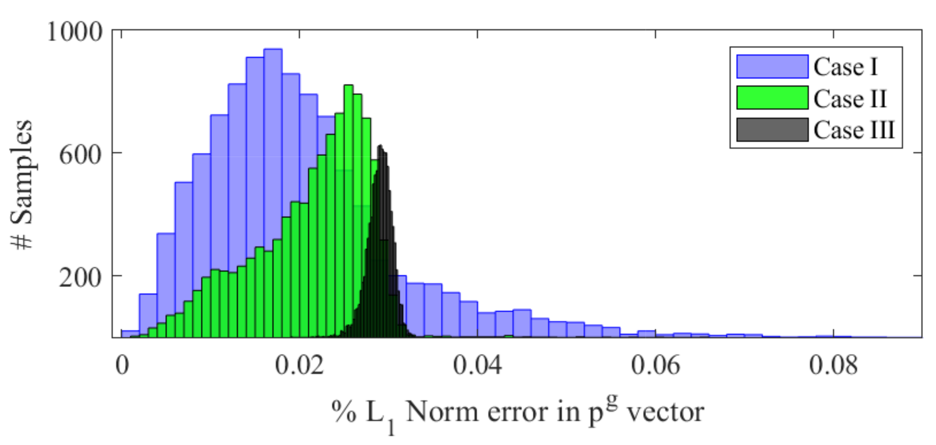
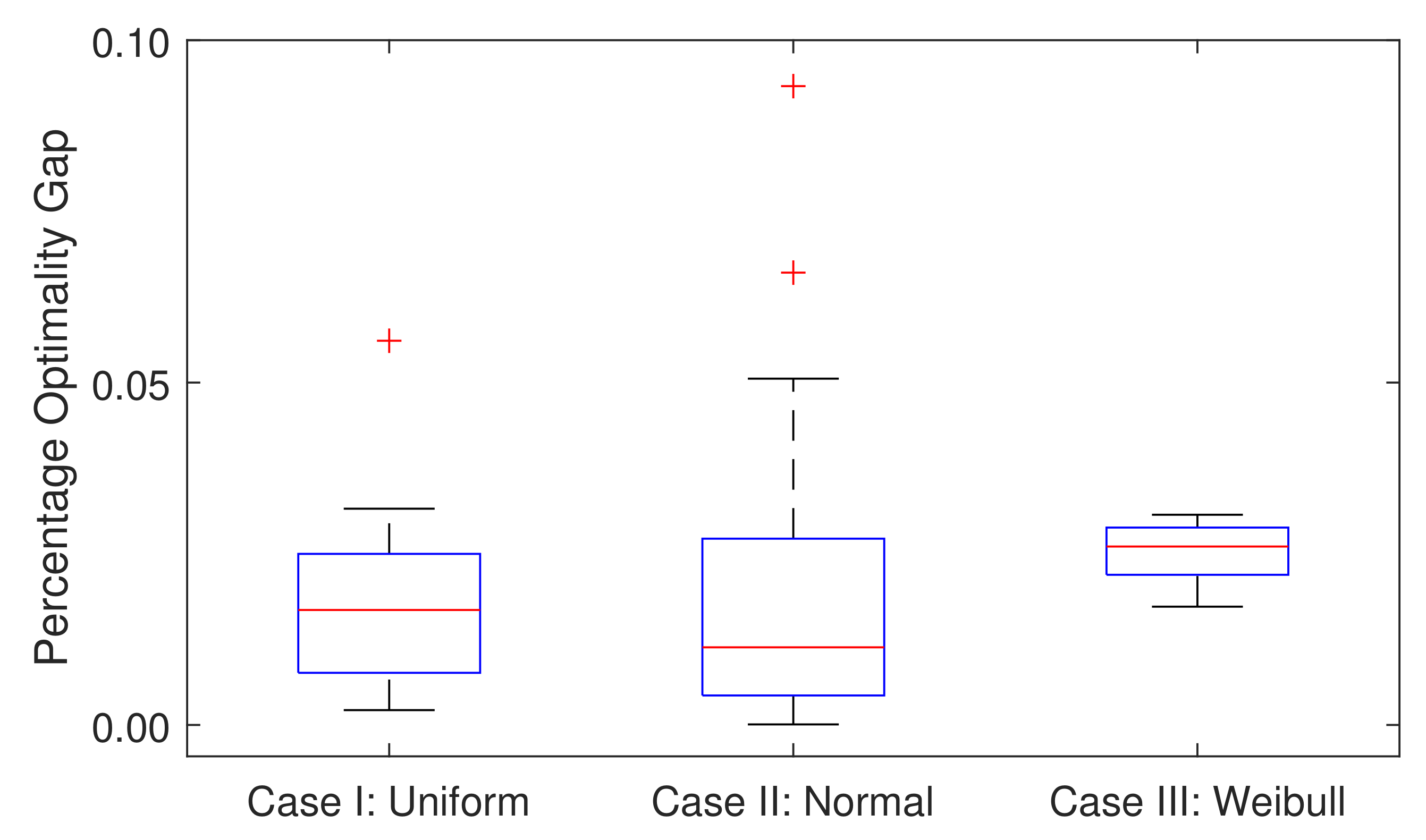
• Case I: Uniform distribution of uncertain net-load vector $\xi$, within $\pm 30\%$ variation of base-load of each node;
• Case II: Normal distribution of uncertain net-load vector $\xi$ with base-load as mean and $10\%$ of the base-load taken as standard deviation for each node;
• Case III: Weibull distribution of uncertain net-load vector $\xi$ with base-load selected as scale and $1.5$ times the base-load taken as shape parameter for each node.

It is important to note that we consider the load as net-load, meaning uncertain distributed generation (from renewable sources) is subtracted from the uncertain demand at each node. Therefore, the simulations cases above are explicitly designed to showcase the proposed methods ability to work with both uncertain load and renewable injection together.

Now to show the distribution robustness of RT policy (10), we draw $\%L_1$ error histogram for generation vector in Figure 1 and for voltage vector in Figure 2. The $\%L_1$ error is defined as $\left|\right|\mathbf{v}-{\mathbf{v}}_s{\left|\right|}_1/\left|\right|{\mathbf{v}}_s{\left|\right|}_1\times 100$ with ${\mathbf{v}}_s$ being the true solution obtained via runopf. We use Case I to train the GP and obtain policy for all there cases without retraining of the model again. It is clear that in case I, mean of error histogram is lower than other cases in Figure 1 and Figure 2. Note that the $\%L_1$ norm error in all three cases is <$1\%$. This is indicative of the distributional robustness of the proposed GP-based policy.

The importance of SA-SOPF lies in it’s ability to outperform conventional SOPF in terms of minimizing the expectation of voltage deviation. The

Table 1. SA-SOPF results of change in day-ahead cost, and real-time deviations with respect to day-ahead ACOPF.

	$\Delta \mathit{g}\left({\mathbf{p}}^{\mathit{g}}\right)$	$\Delta \left|\right|{\mathbb{E}}_{\mathit{\xi }}\{\Delta {\mathbf{p}}^{\mathit{g}}\}{\left|\right|}^2$	$\Delta \left|\right|{\mathbb{E}}_{\mathit{\xi }}\{\Delta \mathbf{v}\}{\left|\right|}^2$
Case I	5.7438 $/hr	0.0349 MW	−0.6680 pu
Case II	5.7440 $/hr	0.0189 MW	−0.6672 pu
Case III	5.7721 $/hr	−0.1975 MW	−0.6586 pu

contains the comparison of SA-SOPF results with SOPF for case I–III. It shows that with very less extra cost (<1% of SOPF cost of 6429.31 $/hr), SA-SOPF can significantly reduce the voltage deviation. This evidence suggests that there exist DA optimal solutions, which lead to lower state deviation without a significant increase in the cost.

Further, case I–III have the base-load as the mean ${\mathbf{p}}_o^d=\mathit{\mu }$. This means that DA optimal base-solution without RT objective will lead to the very less value of $\mathbb{E}\{\Delta {\mathbf{p}}^g\}=M_p\mathit{\mu }+C_p$. In other words, the DA scheduling ACOPF solution will be close to the RT optimal solution for generation ${\mathbf{p}}^{g,r}$. Therefore, we test our method’s robustness on a case where the mean of the uncertain load is different from base-load $\mathit{\mu }\ne {\mathbf{p}}_o^d$.

• Case IV: Normal distribution of uncertain net-load vector $\xi$ with $1.1$ times base-load as mean and $10\%$ of the base-load taken as standard deviation for each node.

The case IV is used, as a harsh condition, to show the performance of proposed SA-SOPF formulation to achieve its intended goal of minimization of state-deviation with DA generation cost. The Pareto front between three objective terms of (3) (solved via (19)) for case IV is given in Figure 3 while results comparing numerical values of day-ahead cost based ACOPF and SA-SOPF Pareto solution are given in

Table 2. SA-SOPF results for Case-IV.

	$\mathit{g}\left({\mathbf{p}}_{\mathit{o}}^{\mathit{g}}\right)$	$\left|\right|{\mathbb{E}}_{\mathit{\xi }}\{\Delta {\mathbf{p}}^{\mathit{g}}\}{\left|\right|}^2$	$\left|\right|{\mathbb{E}}_{\mathit{\xi }}\{\Delta \mathbf{v}\}{\left|\right|}^2$
ACOPF	6429.31 $/hr	204.13 MW	0.6709 pu
SA-SOPF-Pareto	6730.55 $/hr	61.92 MW	0.0185 pu
Change	4.685%	−69.66%	−97.24%

. Both these results show that the proposed SA-SOPF formulation achieves an order-of-magnitude lower expectation in voltage deviation, compared with ACOPF results. Further, the reduction in expectation of generation deviation is significant compared to the increase in DA schedule cost. This proves proposed SA-SOPF’s applicability under worst-cases like case IV.

5.2. 30-Bus System

In this subsection, we present the results on 30-bus system [27,28]. This test system has total of six generators and 21 load buses. We consider all 21 loads as random variables, thus effectively having a 21-dimensional vector $\mathsf{\Xi }$. We consider the base-load as 0.8 times of the load given in the data file with [27] to ensure feasibility within the uncertain load space. For learning the affine policy, a load space of ±20% is considered assuming that all the points within this subspace are feasible for ACOPF. We check this assumption by simulating ACOPF for ${10}^4$ samples. For testing, we consider an uncorrelated normal distribution with a 5% standard deviation of base-load for testing this case study.

Figure 4 shows the $\%L_1$ norm error for the generator and voltage magnitude vectors. The affine policy quality is assessed against ${10}^4$ samples of true ACOPF solution. The left sub-figure in the Figure 4 shows that the affine policy learned using GP has $\%L_1$ norm error less than 0.03%. This indicates that the proposed method has been able to approximate the relationship accurately. The error plot for $\left|V\right|$ shows that the percentage error in the voltage magnitude is of the order of ${10}^{-3}$ which is considerably low.

Table 3. SA-SOPF results for 30-bus system.

	$\mathit{g}\left({\mathbf{p}}_{\mathit{o}}^{\mathit{g}}\right)$	$\left|\right|{\mathbb{E}}_{\mathit{\xi }}\{\Delta {\mathbf{p}}^{\mathit{g}}\}{\left|\right|}^2$	$\left|\right|{\mathbb{E}}_{\mathit{\xi }}\{\Delta \mathbf{v}\}{\left|\right|}^2$
ACOPF	388.22 $/h	17.305 MW	0.087818 pu
SA-SOPF-Pareto	392.86 $/h	1.716 MW	$7.43\times {10}^{-5}$ pu
Change	1.195%	−90.08%	−99.915%

shows the results of the proposed SA-SOPF Pareto optimal with the ACOPF results with perfect information. It shows that with $1.195\%$ extra cost, there is $90.08\%$ reduction in the expectation generator set-point deviation. Further, the expectation in the change in voltage deviation has also been reported as $99.91\%$ in the Table 3.

For indicating the increase in the generation cost due to different penalties, we present the Pareto front for considering all three objective terms in Figure 5. The figure shows that a significant decrease in the deviation of generation set-points is obtained, at the expense of cost and voltage set-point deviation increase. However, the cost increment of approximately 1% for Pareto optimal shows a possibility of obtaining the low state deviation solution compared with a very low-cost increase.

5.3. Optimality Gap and Computation Time

An aspect of the policy accuracy is the optimality gap between the solutions obtained using the proposed affine policy and perfect information ACOPF solution. There will be a non-zero optimality gap in most of the conditions due to non-linearity of power flow manifold. In Figure 6 we present a box plot representing the percentage optimality gap between the cost obtained using affine policy and true, complete information ACOPF. It is clear that affine policy has achieved a significantly less optimality gap (<0.1%) for all three cases. This shows that the affine decision rule is a highly accurate approximation of the actual decision rule, in distributionally robust manner.

Table 4. Computation time for various case studies.

System	Learning (s) ${\mathbf{p}}^{\mathit{g}}+\mathbf{v}$	SA-SOPF (s)
14-bus	2.41 + 16.88 = 19.29	0.157
30-bus	4.01 + 38.01 = 42.02	2.325

contains the results for the time taken in learning voltage and generation set-point affine policy. The table also shows the time taken to solve the SA-SOPF problem using MOSEK 9.2 with YALMIP [29] on MATLAB R2020b. The time is given in seconds. All the simulations are performed using the GPML toolbox [30] on PC having Intel Xeon [email protected] GHz, 16 GB RAM. These time results show that the proposed method has obtained the DR affine policy for different systems within 1 min, and the SA-SOPF solution is obtained in negligible time. We use only 450 ACOPF training samples, which makes the proposed method computationally-lite compared to large-scale MCS-based methods. Importantly, the proposed work focuses on finding an affine recourse policy and a solution to the SOPF problem, minimizing the cost and the state deviation for a future scheduling period. This future scheduling period can be a few hours ahead or a day ahead. We do not propose the SA-SOPF problem solving or distributionally robust affine policy learning in real-time. Therefore, the time taken by the proposed method has much less significant as the framework under which the SA-SOPF problem is solved is not time-constrained. We will explore the possibilities of using the scalable Gaussian process learning methods in future works for large-scale systems.

6. Conclusions

A novel state-aware stochastic optimal power flow (SA-SOPF) problem is formulated and solved using convex relaxation. The proposed SA-SOPF problem minimizes the day-ahead generation schedule cost and expectation of deviation in generation and voltage for ACOPF under uncertainty. The recourse function or policy to shift the generation and voltage set-point with load uncertainty are obtained using GP learning—the proposed method results in a distributionally robust affine policy. The policy has produced accurate results for different types of load uncertainty distribution with <$1\%L_1$ error. The proposed formulation is able to minimize the expectation of generation and voltage deviation significantly $>60\%$. The additional day-ahead cost is not more than $5\%$ for 14-bus system. The proposed SA-SOPF attains at least 90% reduction in expectation of set-point variation with only 1.195% extra generation cost for 30-bus system. Therefore, the proposed formulation opens up the possibility of obtaining SOPF solutions, which improves system performance in real-time. The lower state variation in real-time will lead to lower power flow change, lower locational marginal price change, and fewer control operations requirements like tap changing. Future work will explore the possibilities of combining the policy learning and optimization problem. The problem learning of distributionally robust affine policy for larger systems will also be considered in future.

References

1. Mezghani, I.; Misra, S.; Deka, D. Stochastic AC optimal power flow: A data-driven approach. Electr. Power Syst. Res. 2020, 189, 106567. [Google Scholar] [CrossRef]
2. Dandurand, B.; Kim, K.; Schanen, M. Toward a scalable robust security-constrained optimal power flow using a proximal projection bundle method. Electr. Power Syst. Res. 2020, 189, 106681. [Google Scholar] [CrossRef]
3. Baker, K.; Toomey, B. Efficient relaxations for joint chance constrained AC optimal power flow. Electr. Power Syst. Res. 2017, 148, 230–236. [Google Scholar] [CrossRef] [Green Version]
4. Arrigo, A.; Ordoudis, C.; Kazempour, J.; De Grève, Z.; Toubeau, J.F.; Vallée, F. Optimal Power Flow Under Uncertainty: An Extensive Out-of-Sample Analysis. In Proceedings of the 2019 IEEE PES Innovative Smart Grid Technologies Europe (ISGT-Europe), Bucharest, Romania, 29 September–2 October 2019; pp. 1–5. [Google Scholar]
5. Yong, T.; Lasseter, R. Stochastic optimal power flow: Formulation and solution. In Proceedings of the Power Engineering Society Summer Meeting, Seattle, WA, USA, 16–20 July 2000; Volume 1, pp. 237–242. [Google Scholar]
6. Roald, L.; Andersson, G. Chance-constrained AC optimal power flow: Reformulations and efficient algorithms. IEEE Trans. Power Syst. 2017, 33, 2906–2918. [Google Scholar] [CrossRef] [Green Version]
7. Vrakopoulou, M.; Margellos, K.; Lygeros, J.; Andersson, G. A Probabilistic Framework for Reserve Scheduling and N-1 Security Assessment of Systems with High Wind Power Penetration. IEEE Trans. Power Syst. 2013, 28, 3885–3896. [Google Scholar] [CrossRef]
8. Mühlpfordt, T.; Faulwasser, T.; Hagenmeyer, V. Solving stochastic ac power flow via polynomial chaos expansion. In Proceedings of the IEEE Conference on Control Applications (CCA), Buenos Aires, Argentina, 19–22 September 2016; pp. 70–76. [Google Scholar]
9. Louca, R.; Bitar, E. Stochastic AC optimal power flow with affine recourse. In Proceedings of the IEEE 55th CDC, Las Vegas, NV, USA, 12–14 December 2016; pp. 2431–2436. [Google Scholar]
10. Baghsorkhi, S.S.; Hiskens, I.A. Impact of wind power variability on sub-transmission networks. In Proceedings of the IEEE PESGM, San Diego, CA, USA, 22–26 July 2012. [Google Scholar]
11. Bienstock, D.; Shukla, A. Variance-aware optimal power flow: Addressing the tradeoff between cost, security, and variability. IEEE Trans. Control. Netw. Syst. 2019, 6, 1185–1196. [Google Scholar] [CrossRef]
12. Molzahn, D.K.; Roald, L.A. Towards an AC optimal power flow algorithm with robust feasibility guarantees. In Proceedings of the 2018 Power Systems Computation Conference (PSCC), Dublin, Ireland, 11–15 June 2018; pp. 1–7. [Google Scholar]
13. Mieth, R.; Dvorkin, Y. Data-driven distributionally robust optimal power flow for distribution systems. IEEE Control Syst. Lett. 2018, 2, 363–368. [Google Scholar] [CrossRef] [Green Version]
14. Louca, R.; Bitar, E. Robust AC optimal power flow. IEEE Trans. Power Syst. 2018, 34, 1669–1681. [Google Scholar] [CrossRef] [Green Version]
15. Lorca, A.; Sun, X.A. The Adaptive Robust Multi-Period Alternating Current Optimal Power Flow Problem. IEEE Trans. Power Syst. 2018, 33, 1993–2003. [Google Scholar] [CrossRef]
16. Guo, Y.; Baker, K.; Dall’Anese, E.; Hu, Z.; Summers, T.H. Data-based distributionally robust stochastic optimal power flow—Part I: Methodologies. IEEE Trans. Power Syst. 2018, 34, 1483–1492. [Google Scholar] [CrossRef] [Green Version]
17. Venzke, A.; Halilbasic, L.; Markovic, U.; Hug, G.; Chatzivasileiadis, S. Convex relaxations of chance constrained AC optimal power flow. IEEE Trans. Power Syst. 2017, 33, 2829–2841. [Google Scholar] [CrossRef] [Green Version]
18. Birge, J.R.; Louveaux, F. Introduction to Stochastic Programming; Springer Science & Business Media: Berlin/Heidelberg, Germany, 2011. [Google Scholar]
19. Lavaei, J.; Low, S.H. Zero duality gap in optimal power flow problem. IEEE Trans. Power Syst. 2012, 27, 92–107. [Google Scholar] [CrossRef] [Green Version]
20. Williams, C.K.; Rasmussen, C.E. Gaussian Processes for Machine Learning; MIT Press: Cambridge, MA, USA, 2006; Volume 2. [Google Scholar]
21. Pareek, P.; Nguyen, H.D. Probabilistic robust small-signal stability framework using Gaussian process learning. Electr. Power Syst. Res. 2020, 188, 106545. [Google Scholar] [CrossRef]
22. Pareek, P.; Yu, W.; Nguyen, H. Optimal Steady-state Voltage Control using Gaussian Process Learning. IEEE Trans. Ind. Inform. 2020. [Google Scholar] [CrossRef]
23. Wiesemann, W.; Kuhn, D.; Sim, M. Distributionally robust convex optimization. Oper. Res. 2014, 62, 1358–1376. [Google Scholar] [CrossRef]
24. Pareek, P.; Nguyen, H.D. Gaussian Process Learning-based Probabilistic Optimal Power Flow. IEEE Trans. Power Syst. 2021, 36, 541–544. [Google Scholar] [CrossRef]
25. Coffrin, C.; Hijazi, H.L.; Van Hentenryck, P. Strengthening the SDP relaxation of AC power flows with convex envelopes, bound tightening, and valid inequalities. IEEE Trans. Power Syst. 2016, 32, 3549–3558. [Google Scholar] [CrossRef]
26. Pareek, P.; Nguyen, H.D. A Convexification Approach for Small-Signal Stability Constrained Optimal Power Flow. IEEE Trans. Control of Network Syst. 2021. [Google Scholar] [CrossRef]
27. Zimmerman, R.D.; Murillo-Sánchez, C.E.; Thomas, R.J. MATPOWER: Steady-state operations, planning, and analysis tools for power systems research and education. IEEE Trans. Power Syst. 2010, 26, 12–19. [Google Scholar] [CrossRef] [Green Version]
28. Madani, R.; Sojoudi, S.; Lavaei, J. Convex relaxation for optimal power flow problem: Mesh networks. IEEE Trans. Power Syst. 2014, 30, 199–211. [Google Scholar] [CrossRef]
29. Löfberg, J. YALMIP : A Toolbox for Modeling and Optimization in MATLAB. In Proceedings of the CACSD Conference, Taipei, Taiwan, 2–4 September 2004. [Google Scholar]
30. Rasmussen, C.E.; Nickisch, H. Gaussian processes for machine learning (GPML) toolbox. J. Mach. Learn. Res. 2010, 11, 3011–3015. [Google Scholar]
Figure 1. % L 1 norm error in p g for 10 4 sample MCS.
Sustainability 13 07577 g001
Figure 2. % L 1 norm error in | V | for 10 4 sample MCS.
Sustainability 13 07577 g002
Figure 3. Pareto for Case-IV (14-bus system), points within ellipse are of minimum distance from origin, i.e., Pareto optimal.
Sustainability 13 07577 g003
Figure 4. % L 1 -norm error in p g and | V | in 30-Bus system calculated with 10 4 sample MCS.
Sustainability 13 07577 g004
Figure 5. Pareto for 30-Bus, points within ellipse are of minimum distance from origin i.e., Pareto optimal.
Sustainability 13 07577 g005
Figure 6. Percentage optimality gap between the cost of generation using true, complete information ACOPF and affine policy in (8) for IEEE 14-bus system. The test is conducted three different cases with 10 4 samples. The cost coefficients are taken from [27].
Sustainability 13 07577 g006