Research on a Visual Comfort Model Based on Individual Preference in China through Machine Learning Algorithm

Abstract

Recently, decreasing energy consumption under the premise of building comfort has become a popular topic, especially visual comfort. Existing research on visual comfort lacks a standard of how to select indicators. Moreover, studies on individual visual preference considering the interaction between internal and external environment are few. In this paper, we ranked common visual indicators by the cloud model combined with the failure mode and effect analysis (FMEA) and hierarchical technique for order of preference by similarity to ideal solution (TOPSIS). Unsatisfied vertical illuminance, daylight glare index, luminance ratio, and shadow position are the top four indicators. Based on these indicators, we also built the individual visual comfort model through five categories of personalized data obtained from the experiment, which was trained by four machine learning algorithms. The results show that random forest has the best prediction performance and support vector machine is second. Gaussian mixed model and classification tree have the worst performance of stability and accuracy. In addition, this study also programmed a BIM plug-in integrating environmental data and personal preference data to predict appropriate vertical illuminance for a specific occupant. Thus, managers can adjust the intensity of artificial light in the office by increasing or decreasing the height of table lamps, saving energy and improving occupant comfort. This novel model will serve as a paradigm for selecting visual indicators and make indoor space be tailored to meet individual visual preferences.

1. Introduction

Buildings, where people live, are closely related to the lives of people. People usually spend approximately 90% of their time living in buildings [1]. Generally, energy consumed by buildings accounts for about 40% of global energy consumption. According to a report of the Joint Research Center of the European Union, the energy consumption for artificial lighting accounts for 14% in the EU and 19% in the world [2]. In 2018, the energy consumption of China’s construction industry was 2.147 billion tce, accounting for 46.5% of China’s total energy consumption. During the operation and maintenance, energy consumption was 1 billion tce, which accounts for 46.6% of the energy consumption of the building industry [3]. As a prominent building system, the lighting system consumes approximately 14% of energy in the operation phase. Therefore, reducing the energy consumption of the lighting system signifies reducing the overall energy consumption of the building. The latest Plan for the 14th Five-Year Plan of China puts forward the goal of “carbon neutrality”, which reflects the determination and urgent need to reduce carbon emissions. Consequently, energy consumption in the building sector must be reduced.

With the continuous development of the economy, people have raised the requirements for indoor rooms and pay more attention to the comfort of living. As a part of the indoor environment, visual comfort is an integral part of building energy consumption, personal health, work efficiency, and satisfaction, which has also attracted many scholars [4]. In the interior environment of buildings, individuals have preferences for visual environment [5,6,7]. Research has confirmed that when occupants can adjust the illuminance of task area, it positively affects satisfaction with environmental conditions [8], the quantity and quality of lighting [9], mood [10], and productivity [11]. Since different individuals may change the intensity of light in different periods and different scenarios, a unified lighting environment may not meet the needs of different individuals.

In modern society, an increasing number of buildings are designed with highly glazed facades. Featuring the characteristics of design, excessive daylight brings glare to occupants [11]. To solve the visual obstacles caused by natural lighting, Goovaerts C developed a controlling strategy based on occupants’ comfort requirements, which utilized natural lighting to reduce energy consumption [12]. Daylight glare index (DGI) and daylight glare probability (DGP) were used to evaluate daylight glare. Nonetheless, both of them should not be used as variables to assess discomfort independently [13]. In addition, some research concluded that vertical illuminance is better than common indicators such as horizontal illuminance, luminance ratio, and DGI [14]. Although preventing glare is essential, achieving general visual comfort will not be satisfied with the optimal visual environment [5]. In contrast, without only applying glare, considering individual preference may lead to optimizing the visual environment.

Recent studies mostly focus on assessing visual discomfort in daylight space by applying visual discomfort metrics including complex fenestration systems [15], automated shade systems [16,17], and variations in luminance type [18]. However, most studies consider the perspective of overall buildings or interior space rather than occupant individual preferences. In fact, learning personalized visual lighting for indoor daylight control is a challenge. Using a single indicator such as vertical illuminance or DGI is insufficient, especially when occupants work in a public office. Accordingly, we integrated the commonly referred to indicators rather than a single indicator to build the visual model, which would be more accurate and rigorous.

During the operation of smart buildings, some studies have emphasized personalized comfort [19]. A study of occupant-centric lighting approaches by Bakker et al. found that utilizing lighting control approaches developed in the cubicle office may impact occupant satisfaction negatively [20]. It suggested that future research should concentrate on dynamic individual-occupancy patterns, which can be applied to the multi-occupant open office. Thus, meeting individual satisfaction is a challenging problem because acquiring and handling dynamic data about individual visual comfort is difficult. Nevertheless, machine learning and big data mining, treated as the measure to solve the problem, can retrieve useful information from massive data. Some studies use public data to develop data-driven models to infer occupant preferences [21].

In prior glare research, all indicators were reported regardless of whether the indicators were appropriate [22]. Hence, this study mainly completed two tasks. First, it ranked the relative indicators among excessive visual indicators and chose the indicators most relevant to occupant cognition. Second, this study took data from sensors and occupants as inputs and suitable vertical illuminance as output to learn individual visual preference.

In this paper, our contribution to the literature is threefold. First, we contribute to adopting an improved cloud model combining failure mode and effect analysis and hierarchical technique for order of preference by similarity to ideal solution (CMTOPSIS-FMEA) to rank indicators that affect the visual comfort of occupants. Second, through the visual satisfaction experiment, we obtained data about favoring of light sources by different individuals and used four types of machine learning algorithms to train models. We also used confusion matrix and area under the curve (AUC) with its standard deviation to assess prediction performance, and the results indicate that random forest (RF) had the best prediction performance. Finally, this study also set up a plug-in program to verify our model. The program uses an individual visual comfort model trained by RF to predict appropriate vertical illuminance, which can help managers adjust the light source intensity in the office and improve the satisfaction of users.

In the next section, a literature review on the visual comfort model is presented. The third section introduces the proposed method and procedure. Then, the results and a case study are used to validate this method in the fourth section. The fifth section discusses the results in detail. Finally, conclusions are offered in the last section.

2. Literature Review

2.1. Visual Comfort Index

In current studies, indexes about visual comfort are excessive, and how to select them correctly becomes a complicated matter. Generally, vertical illuminance outperforms common visual comfort metrics, including horizontal illuminance, luminance ratio, daylight glare probability (DGP), and daylight glare index (DGI) [13]. The correlation between both vertical illuminance and horizontal illuminance on the desk and the users’ perception of glare in the office environment has been confirmed to be statistically significant [23]. In contrast, Kyle Konis used a repeated-measures study to collect subjective measurements of visual comfort. The results show that discomfort indicators based on luminance ratio and absolute measures are more effective than glare metrics or basic vertical or horizontal illuminance measurement [24].

On the other hand, follow-up studies found that the performance of DGI in measuring artificial lighting is not as good as the performance of natural glare [25]. Thus, the CIE glare index (CGI) and unified glare index (UGR) were used to evaluate indoor artificial lighting glare. To analyze DGI and CGI, JA Jakubiec introduced the “adaptive zone”. Applying the “adaptive zone” to offices with manually operated venetian blinds reduces the estimated glare time from 735 to 18 h every year and increases the average annual daylight availability from 40% to 72% [26].

Moreover, a new index, UGP, which is applicable to open-plan green buildings [27], has been developed by investigating discomfort glare with 493 surveys. In addition, Kevin G. compared existing and emerging discomfort glare metrics and suggested potential future research to minimize glare discomfort while promoting occupant visual preferences and whole-building energy efficiency [28]. In summary, considering the timing of the proposal and its simple calculation process, DGI is still the leading indicator that most researchers pay attention to.

There are two main limitations in the field of visual comfort indexes. On the one hand, although excessive indicators are affecting indoor visual comfort, the standard of selection and evaluation of indicators is ambiguous and lacks a clear explanation of how to select appropriate indicators under different situations. In recent studies, whether the indicators are appropriate or not, commonly referred to indicators involved are reported in the paper [22]. On the other hand, the main content and parameters between the two indexes are the same. Consequently, establishing an appropriate and comprehensive visual index system is necessary.

2.2. Visual Comfort Model

According to the previous research of scholars, there is a ravine between the lighting preference profiles of users. When faced with an uncomfortable office environment, many occupants hesitate to take action to cause discomfort to colleagues [16]. The comfort of the light environment is a part of the building’s overall comfort and is vital for the user’s indoor experience. Therefore, building models for individual needs and using the trained model to calculate indoor light illuminance toward specific individuals helps the visual environment preference.

Some scholars use natural lighting to reduce visual glare and building energy consumption while other scholars also directly develop software to reduce energy consumption during operation and maintenance. Yonggang Zhang et al. used particle swarm optimization to optimize curtain coverage, thereby putting in natural light to improve the indoor comfortable visual environment [11]. Nonetheless, because the light environment comfort cannot be accurately quantified, the accuracy of the model is barely satisfactory. Thus, Jie Xiong et al. deduced a personalized visual satisfaction model in a private office through Bayesian analysis to coordinate personal satisfaction and energy savings [5]. However, the data needed for the training model are not well explained in this paper, such as how many data points are needed to complete the training of the personalized visual satisfaction model or what types of data and indicators are needed for training. Toward this, Kar et al. built a recommendation system for intelligently controlling the lighting system, ReViCEE, by collecting historical data such as an individual and overall preference for the light environment [29]. This paper told us the amount of data but did not answer the question of what types of data and indicators.

Apart from instantaneous visual comfort, a study aimed at long-term visual impression was designed to record four visual discomfort types: discomfort glare, insufficient monitor contrast, direct visibility of the sun, and direct sunlight on the workplane. The conclusions confirmed that it is feasible to use the current simulation-based prediction method of visual comfort to predict occupants’ long-term visual comfort [30].

2.3. Solar Shading System

Natural lighting, a medium of contact between occupants and the external environment, improves work efficiency and visual satisfaction [31]. However, circumstances still exist in which occupants change workplaces due to daylight glare [32]. Consequently, as an effective measure to resist natural light, solar shading systems have received much attention. Simultaneously, considering that the demand for energy during operation and maintenance is increasing rapidly, solar shading systems can improve occupant comfort while making full use of natural lighting [33]. Researchers focus on dynamically controlling shading devices to reduce building energy costs and improve thermal comfort of interior space.

To quantify the potential of dynamic solar shading facade components, Littlefair et al. used a simulation study to investigate three facade types: without shading, with fixed shading, and with dynamic shading [34]. Nielsen et al. compared manually controlled internal blinds, fixed externally hung blinds, and internal or external blinds under automatic control and manual override in the UK and found that a shading system can reduce carbon dioxide emissions and energy costs [35]. Palmero et al. used TRNSYS simulation to investigate the building energy-saving performance for louver shading systems in Mexico, Cairo, Lisbon, Madrid, and London [36]. The results show that the application of the louver shading system can make the indoor thermal environment more comfortable and the energy-saving effect is more significant.

Considerable research efforts with comprehensive coverage have been devoted to comfort in the indoor environment. There are also many shortcomings. First, the indexes of glare are excessive and similar, resulting in academics not choosing an appropriate index. Second, the literature is concerned mostly with thermal comfort or solar shading and, to a lesser extent, with satisfaction with the indoor environment. Third, it is considerably challenging to conduct quantitative analysis and calculation because of the subjectivity of the comfort sensation. Moreover, previous literature has focused mainly on reducing building energy consumption and lacks research on building energy efficiency from the perspective of occupants’ preference for the light environment.

The factors affecting visual comfort are varied and perform significantly differently. The CMTOPSIS-FMEA method helps to support the reasoning and expression of expert opinions and is suitable for determining the rankings in various factors. Therefore, before constructing the individual visual comfort model, it is necessary to discuss its importance to personnel’s visual comfort to select the appropriate factors.

3. Method

3.1. Rankings of Indicators of Visual Comfort

There are so many factors of visual comfort that ranking factors is a necessary process before building an individual model. The cloud model, a new uncertainty model based on probability and fuzzy set theory, enables the translation of subjective assessment information to a quantified set or matrix [37]. FMEA is a qualitative analysis method to quantify the risk degrees, which can analyze the possible failure modes and calculate the possible cost. Generally, fuzzy set theory is integrated with multi-criteria decision making (MCDM) to improve traditional FMEA [38]. Due to the fuzziness of FMEA team assessments, it cannot express the randomness of team assessment. Therefore, the cloud model can solve the fuzziness, hesitation, and randomness of expert assessments [39].

Linguistic variable is an effective tool to flexibly express uncertain definitions or complex situations, which is difficult to accurately express by quantitative values [40]. Thus, experts prefer to apply fuzzy linguistic variables to express their judgments [41]. Meanwhile, using TOPSIS to solve the MCDM problem is justified because it can provide corresponding decision matrix and rank relevant factors [42,43]. In general, combined with the FMEA and TOPSIS method, the cloud model can be integrated to calculate the ranking of the factors that affect visual comfort [44]. This method solves the dilemma of uncertain and ambiguous assessment information, which is a logical method to quantify the factors’ importance [45]. In this study, visual comfort is considered a project’s success and the indicators adverse to success are considered failure modes.

Indicators of visual comfort in light environments have been proposed in previous studies. Generally, as shown in

Table 1. FMEA of the visual comfort.

Groups	Failure Modes	Symbol
Amount of light	Unsatisfied Vertical Illuminance	FM1
	Unsatisfied Horizontal Illuminance	FM2
	Useful Daylight Illuminance	FM3
Glare	Luminance Ratio	FM4
	Daylight Glare Index	FM5
	Unified Glare Rating	FM6
	Predicted Glare Sensation Vote	FM7
Uniformity of light	Shadow Position	FM8
Quality of light in rendering colors	Color Discrimination Index [54]	FM9
	Color Quality [55]	FM10

, the indicators are divided into four categories: amount of light, glare, uniformity of light, and quality of light [46,47]. Amount of light means an adequate amount of light allowing occupants to fulfill the tasks, and uniformity of light refers to the uniform distribution of light in the task area. Glare reflects a phenomenon that makes it difficult to see the surrounding environment because of too bright artificial or natural lighting for occupants. Quality of light in rendering colors describes the ability of light to render colors. In other words, it represents the level of similarity to natural light because people prefer natural light in the workspace [48]. In recent years, scholars have focused mainly on indexes for judging and assessing glare and the amount of light. Among 34 indexes recorded in the literature review and the standard, 50% (17/34) of the indexes are appropriately glare, while 26% (9/34) are amount of light. Hence, indexes of glare and amount of light were adopted more than other indexes in this study.

Several variables and their combinations were considered to perceive the visual conditions in the room, which can reflect the accuracy of the subject’s feelings [49]. Vertical and horizontal illuminance refer to the illuminance in both directions of the working area. The technical standard stipulates that the value of vertical and horizontal illuminance set at 300 lux is suitable [47]. Useful daylight illuminance refers to the daylight illuminance in the range of 100–2000 lux, which is considered useful to the illuminance of space [50]. The daylight glare index is the degree of glare discomfort due to sky seen through a window [51]. When the value is greater than 18, the environment is glare. Unified Glare Rating is a psychological parameter used to measure the subjective feeling of light in the indoor visual environment to the discomfort of occupants, and 13 is the boundary of glare [52]. The luminance ratio is the ratio of the average luminance of the window divided by the average luminance of the target surfaces, and the thresholds are defined ranging from 5:1 to 40:1 [53]. Color quality is defined as the effect of illuminance on the color appearance of objects by conscious and subconscious comparison with color performance under the reference illuminance.

In the FMEA model, to confirm the reliability and effectiveness of the failure modes, many qualitative and quantitative risk factors need to be considered. Specifically, severity is divided into five parts. Detection shows two measures while occurrence only has one risk factor (

Table 2. Weight of dimensions and risk factors.

Dimensions	Weight	Risk Factors	Weight	Final Weight
Occurrence	0.270	Frequency (RF1)	1.000	0.270
Severity	0.400	Physiological Comfort (RF2)	0.300	0.120
		Psychological Comfort (RF3)	0.333	0.133
		Work Efficiency (RF4)	0.267	0.107
		Energy Consumption (RF5)	0.067	0.027
		Environment (RF6)	0.033	0.013
Detection	0.330	Supervisory (RF7)	0.700	0.231
		Visible (RF8)	0.300	0.099

).

3.1.1. Translate Fuzzy Assessment Information into a Cloud

Suppose that the effective domains $\text{U}= \left[X_{min}, X_{max}\right] = \left[0,10\right]$ and $\mathrm{S}= \left\{{\mathrm{s}}_0,{\mathrm{s}}_1,\dots ,{\mathrm{s}}_8\right\}$ is an assessment information set. Thus, m + 1 basic cloud is generated through Formulas (1)–(9).

$$\begin{array}{c}\mathrm{S}=\{{\mathrm{s}}_0=\mathrm{Absolutely}\mathrm{Low}\left(\mathrm{AL}\right),{\mathrm{s}}_1=\mathrm{Very}\mathrm{Low}\left(\mathrm{VL}\right),{\mathrm{s}}_2=\mathrm{Low}\left(\mathrm{L}\right),{\mathrm{s}}_3=\mathrm{Moderately}\mathrm{Low}\left(\mathrm{ML}\right),{\mathrm{s}}_4\\ \hspace{0.17em}\hspace{0.17em}\hspace{0.17em}\hspace{0.17em}\hspace{0.17em}\hspace{0.17em}\hspace{0.17em}\hspace{0.17em}\hspace{0.17em}\hspace{0.17em}\hspace{0.17em}\hspace{0.17em}\hspace{0.17em}\hspace{0.17em}\hspace{0.17em}=\mathrm{Moderate}\left(\mathrm{M}\right),{\mathrm{s}}_5=\mathrm{Moderately}\mathrm{High}\left(\mathrm{MH}\right),{\mathrm{s}}_6=\mathrm{High}\left(\mathrm{H}\right),{\mathrm{s}}_7=\mathrm{Very}\mathrm{High}\left(\mathrm{VH}\right),{\mathrm{s}}_8\\ \hspace{0.17em}\hspace{0.17em}\hspace{0.17em}\hspace{0.17em}\hspace{0.17em}\hspace{0.17em}\hspace{0.17em}\hspace{0.17em}\hspace{0.17em}\hspace{0.17em}\hspace{0.17em}\hspace{0.17em}\hspace{0.17em}\hspace{0.17em} =\mathrm{Absolutely}\mathrm{High}\left(\mathrm{AH}\right)\}\hfill \end{array}$$

E_x is the expectation, representing the central value of qualitative linguistic concept field. E_n represents entropy and is used to describe the randomness of qualitative linguistic concepts. H_e is hyper entropy, which reflects the uncertainty. Then, H_e4 = 0.04 [45] and basic clouds are calculated and the numerical characteristics are stated as follows:

$${\tilde{\mathrm{y}}}_0=({\mathrm{E}}_{\mathrm{x}0},{\mathrm{E}}_{\mathrm{n}0},{\mathrm{H}}_{\mathrm{e}0})=\left({\mathrm{X}}_{\min }+3{\mathrm{E}}_{\mathrm{n}0},\frac{{\mathrm{E}}_{\mathrm{n}1}}{0.618},\frac{{\mathrm{H}}_{\mathrm{e}1}}{0.618}\right)=\left(2.619,0.873,0.275\right)$$

(1)

$${\tilde{\mathrm{y}}}_1=({\mathrm{E}}_{\mathrm{x}1},{\mathrm{E}}_{\mathrm{n}1},{\mathrm{H}}_{\mathrm{e}1})=\left({\mathrm{E}}_{\mathrm{x}2}-0.382\left({\mathrm{E}}_{\mathrm{x}2}-{\mathrm{E}}_{\mathrm{x}0}\right),\frac{{\mathrm{E}}_{\mathrm{n}2}}{0.618},\frac{{\mathrm{H}}_{\mathrm{e}2}}{0.618}\right)=\left(3.181,0.539,0.170\right)$$

(2)

$${\tilde{\mathrm{y}}}_2(={\mathrm{E}}_{\mathrm{x}2},{\mathrm{E}}_{\mathrm{n}2},{\mathrm{H}}_{\mathrm{e}2})=\left({\mathrm{E}}_{\mathrm{x}3}-0.382\left({\mathrm{E}}_{\mathrm{x}3}-{\mathrm{E}}_{\mathrm{x}0}\right),\frac{{\mathrm{E}}_{\mathrm{n}3}}{0.618},\frac{{\mathrm{H}}_{\mathrm{e}3}}{0.618}\right)=\left(3.528,0.333,0.105\right)$$

(3)

$${\tilde{\mathrm{y}}}_3=({\mathrm{E}}_{\mathrm{x}3},{\mathrm{E}}_{\mathrm{n}3},{\mathrm{H}}_{\mathrm{e}3})=\left({\mathrm{E}}_{\mathrm{x}4}-0.382\left({\mathrm{E}}_{\mathrm{x}4}-{\mathrm{E}}_{\mathrm{x}0}\right),\frac{{\mathrm{E}}_{\mathrm{n}4}}{0.618},\frac{{\mathrm{H}}_{\mathrm{e}4}}{0.618}\right)=\left(4.090,0.206,0.065\right)$$

(4)

$${\tilde{\mathrm{y}}}_4=({\mathrm{E}}_{\mathrm{x}4},{\mathrm{E}}_{\mathrm{n}4},{\mathrm{H}}_{\mathrm{e}4})=\left(\frac{{\mathrm{X}}_{\min }+{\mathrm{X}}_{\max }}{2},0.382\frac{{\mathrm{X}}_{\max }-{\mathrm{X}}_{\min }}{3\left(\mathrm{g}+2\right)},{\mathrm{H}}_{\mathrm{e}4}\right)=\left(5,0.127,0.04\right)$$

(5)

$${\tilde{\mathrm{y}}}_5=({\mathrm{E}}_{\mathrm{x}5},{\mathrm{E}}_{\mathrm{n}5},{\mathrm{H}}_{\mathrm{e}5})=\left({\mathrm{E}}_{\mathrm{x}4}+0.382\left({\mathrm{E}}_{\mathrm{x}8}-{\mathrm{E}}_{\mathrm{x}4}\right),\frac{{\mathrm{E}}_{\mathrm{n}4}}{0.618},\frac{{\mathrm{H}}_{\mathrm{e}4}}{0.618}\right)=\left(5.910,0.206,0.065\right)$$

(6)

$${\tilde{\mathrm{y}}}_6=({\mathrm{E}}_{\mathrm{x}6},{\mathrm{E}}_{\mathrm{n}6},{\mathrm{H}}_{\mathrm{e}6})=\left({\mathrm{E}}_{\mathrm{x}5}+0.382\left({\mathrm{E}}_{\mathrm{x}8}-{\mathrm{E}}_{\mathrm{x}5}\right),\frac{{\mathrm{E}}_{\mathrm{n}5}}{0.618},\frac{{\mathrm{H}}_{\mathrm{e}5}}{0.618}\right)=\left(6.472,0.333,0.105\right)$$

(7)

$${\tilde{\mathrm{y}}}_7=({\mathrm{E}}_{\mathrm{x}7},{\mathrm{E}}_{\mathrm{n}7},{\mathrm{H}}_{\mathrm{e}7})=\left({\mathrm{E}}_{\mathrm{x}6}+0.382\left({\mathrm{E}}_{\mathrm{x}8}-{\mathrm{E}}_{\mathrm{x}6}\right),\frac{{\mathrm{E}}_{\mathrm{n}6}}{0.618},\frac{{\mathrm{H}}_{\mathrm{e}6}}{0.618}\right)=\left(6.819,0.539,0.170\right)$$

(8)

$${\tilde{\mathrm{y}}}_8=({\mathrm{E}}_{\mathrm{x}8},{\mathrm{E}}_{\mathrm{n}8},{\mathrm{H}}_{\mathrm{e}8})=\left({\mathrm{E}}_{\mathrm{x}7}+0.382\left({\mathrm{E}}_{\mathrm{x}8}-{\mathrm{E}}_{\mathrm{x}7}\right),\frac{{\mathrm{E}}_{\mathrm{n}7}}{0.618},\frac{{\mathrm{H}}_{\mathrm{e}7}}{0.618}\right)=\left(7.381,0.873,0.275\right)$$

(9)

where ${\tilde{\mathrm{y}}}_{\mathrm{m}}$ indicates basic clouds transformed by nine assessment information sets while X_max and X_min are maximum and minimum values of domain. After getting basic clouds, the ten failure modes were assessed by five members based on their studies and experience. Second, the linguistic evaluation information can be transferred into cloud matrix ${\tilde{\mathrm{y}}}_{\mathrm{m}}$ = (y_ij^m)_10×8 (m = 1,2,…,5) through basic clouds.

3.1.2. Determine the Weights of Experts

In FMEA method, the risk assessment of failure mode always involves multiple team members. Because different experts may have different knowledge and personal preferences, they will express various and subjective views on the same failure mode. The failure modes of visual satisfaction are various and subjective, which is suitable to transform into quantitative set.

To solve the limitations of expert’s bounded rationality, the weight of each expert comes from three different dimensions: professional relevance, experience, and title. The expert weight evaluation table is constructed in

Table 3. Weight allocation table for experts.

Dimensions	Classes	Score
Professional relevance	High	3
	Medium	2
	Low	1
Experience	Over 10 years	3
	5–10 years	2
	Under 5 years	1
Title	Senior	3
	Intermediate	2
	Junior	1

[39,41]. Based on the professional relevance, experience, and title of each expert, the weight is determined by Equation (10).

$${\lambda }_k=\frac{H_k}{{{\displaystyle \sum }}_{k=1}^5{H}_k}, k=1,2,\cdots ,5$$

(10)

where H_k is the score of kth experts and λ_k is the subjective weight. We invited five experts as our responders to score the importance. Experts were university professors engaged in building comfort, designers engaged in interior space design, and managers engaged in dwelling fit-out projects. Thus, they were familiar and proficient in comfort research about the indoor environment, which is authoritative for providing opinions and explanations on the importance of factors. As some experts worked at various locations, considering the convenience of data collection, we used field and online interviews to collect data. Experts on teams had different experiences and knowledge distances in the field of visual comfort, and therefore the weight of each expert was determined by their studies and influence (

Table 4. Weights of the five experts.

Weight	TM1	TM2	TM3	TM4	TM5
Hk	8	4	3	5	6
λk	0.31	0.15	0.11	0.19	0.23

).

3.1.3. Construct the Hierarchical Cloud Matrix

Based on the hierarchical cloud TOPSIS method, the result of experts’ evaluation can be polymerized into a final hierarchical cloud matrix Y = (y_ij)_10×8, which is shown in Appendix B. Because the risk factors were sorted into occurrence, severity, and detection, the final hierarchical matrix can also be divided into three dimensions. Then, combined with the weights of the eight risk factors listed in Table 2, the final weighted hierarchical cloud matrix Y = (y_ij)_10×8 was obtained. Finally, by adding the same dimension, the overall weighted hierarchical cloud matrix can be calculated (in

Table 5. Overall weighted hierarchical cloud matrix.

Failure Modes	O	S	D
FM1	(1.671, 0.152, 0.048)	(2.409, 0.128, 0.040)	(2.156, 0.140, 0.044)
FM2	(1.412, 0.083, 0.026)	(1.610, 0.107, 0.034)	(2.090, 0.123, 0.039)
FM3	(1.157, 0.075, 0.024)	(2.277, 0.159, 0.050)	(1.930, 0.084, 0.027)
FM4	(1.749, 0.134, 0.042)	(2.341, 0.140, 0.044)	(2.044, 0.118, 0.037)
FM5	(1.845, 0.148, 0.047)	(2.399, 0.161, 0.051)	(1.949, 0.080, 0.025)
FM6	(1.487, 0.060, 0.019)	(2.284, 0.091, 0.029)	(1.693, 0.066, 0.021)
FM7	(1.377, 0.071, 0.022)	(2.071, 0.086, 0.027)	(1.336, 0.100, 0.032)
FM8	(1.575, 0.065, 0.021)	(2.373, 0.121, 0.038)	(2.131, 0.127, 0.040)
FM9	(1.070, 0.084, 0.026)	(1.427, 0.178, 0.056)	(1.611, 0.072, 0.023)
FM10	(0.881, 0.132, 0.042)	(1.633, 0.115, 0.036)	(1.361, 0.090, 0.028)

).

After obtaining the overall weighted hierarchical cloud matrix, the next step is defining the cloud positive ideal solution (CPIS) and the cloud negative ideal solution (CNIS). CPIS represents maximizing the scores of all risk factors for each failure mode, while CNIS signifies minimizing the scores. Hence, through formula (10), the value y_t⁺ = max(y_ij’) is instead CPIS A⁺ and y_t⁻ = min(y_ij’) is used as CNIS A⁻. Calculate each failure mode’s distance from A+ and A-, and the closeness coefficient CC_i is calculated by (13). CC_i is a symbol that reveals the risk of failure mode FM_i. In this case, the rank of all failure modes is determined by the closeness coefficient (

Table 6. Closeness coefficients of visual comfort parameters.

	d+	d−	CCi	Rank
FM1	0.241	2.736	0.919	1
FM2	1.494	1.655	0.526	7
FM3	1.294	1.841	0.587	6
FM4	0.376	2.567	0.872	3
FM5	0.378	2.618	0.874	2
FM6	1.269	2.075	0.621	5
FM7	1.897	1.342	0.414	8
FM8	0.526	2.633	0.833	4
FM9	2.578	0.565	0.180	9
FM10	2.701	0.329	0.109	10

). The results show that the most important indicators are unsatisfied vertical illuminance (UVI), daylight glare index (DGI), luminance ratio (LR), and shadow position (SP). Thus, we tend to use these indicators to construct the individual visual comfort model.

A⁺ = {y₁⁺, y₂⁺, …, y_T⁺}, A⁻ = {y₁⁻, y₂⁻, …, y_T⁻}

(11)

$$d_i^{+}={{\displaystyle \sum }}_{t=1}^{T}d(y_{it}^{\prime },y_t^{+})$$

(12)

$$d_i^{-}={\displaystyle \sum }_{t=1}^{T}d(y_{it}^{\prime },y_t^{-}).i=1,2,\dots ,m$$

(13)

$$C{C}_i=\frac{d_i^{-}}{d_i^{-}+d_i^{+}},i=1,2,\dots ,m$$

(14)

3.2. Personal Visual Comfort Environment

3.2.1. Experimental Environment

To determine the preference of the visual environment for the participants, an experiment was designed in a test room with a fully glazed facade located in Shanghai, shown in the Figure 1. The test room is equipped with suspended LED panel sources. Specifically, eight LED panels were installed at a height of 3.2 m. The ceiling height of the laboratory is 3300 mm, while the south-facing facade is almost fully covered by floor-to-ceiling windows, and light-colored slatted blinds are installed in the interior. The window is composed of a single layer of glass with normally visible transmittance of 85%, and the window frame is aluminum alloy. The size of the subject’s desk is 800 mm × 600 mm, the height is 750 mm, perpendicular to the window, and the distance from the window to the top edge of the desk is 1400 mm. Natural light can be illuminated through the window, combining the artificial indoor light source to form the indoor environment. The participants can control the blinds manually to adjust the luminance of natural light. The data such as vertical illuminance and window illuminance can be obtained through field measurement methods.

3.2.2. Participants

Six subjects were recruited in this research, all of whom were undergraduate and graduate Chinese students. The mean age was 23.3 years, and four males and two females were in good health and had normal vision. Since this experiment aimed mainly to influence preferences brought by personalization, it was not necessary to have generality among different individuals and have too many samples. Before the experiment, all subjects were trained in a unified way, including a clear set of instructions such as a definition of discomfort glare. Meanwhile, participants in the experiment were required to have a full rest and not stay up late on the day before to avoid the influence of other factors.

3.2.3. Procedure and Data Collection

The experiment was conducted mainly from 10 October 2020, to 18 March 2021. In this period, the experiments were conducted continuously, the weather was changeable (perhaps sunny, cloudy, or rainy), and the temperature ranged from 28 to −6 °C. According to the conclusion of Christoffersen, there are no real distinctions between seasons evaluation, but time of day needs to be concerned [56]. This paper emphasizes the preference for the lighting environment within a day and does not propose a general model. Considering that the factors affected by seasons are only natural light illuminance, which has little effect on the individual model, it is acceptable to set the experiment in winter and spring.

During the experiment, the subjects worked in front of the desk to read documents with sparse fonts and equal font sizes or electronic documents with monitors at different times. Each hour of work requires a five-minute break for participants to ensure that excludes some factors from the perception of light environment. The Testo 540 illuminance meter (measuring range: 0–99,999 lux, accuracy ≤ 3%) was used to measure the vertical illuminance and horizontal illuminance, and TES 1332A luminance meter (measuring range: 0–200,000 cd/m²) was applied to measure the floor-to-ceiling window luminance and working plane luminance [57]. Every 5 min (aligned with the survey response times), the meters were applied to measure the luminance field on the desk and near the side of the window vertically [58]. Then the average luminance was obtained after three measurements to reduce the error, and the DGI, LR, and other indicators were calculated by the previous results. Students completed relevant questionnaires (Appendix A) to reflect their satisfaction with the light environment and their personal equipment data [59]. The participants scored the overall visual comfort, and the score was divided into 3 degrees (+1, 0, −1), representing from dim to bright for quantitative processing. There is a substantial amount of literature on visual environment evaluation [5], and the three-point scale applied in this study serves to solve the evaluation standard. The mid-point of the scale is “Satisfactory”, which is a diverse type of assessment from judging darkness or brightness. According to Kim’s research, using three levels to solve multiclass classification problems of occupant environmental preferences is better because its result of verifying individual preferences is realistic [60].

Through the experiment, we collected five categories of data: (1) Survey data: the subjects completed the survey every time to report their visual acceptability, visual preference, work property, and glasses wearing. (2) Time data: the time of experiment including the hour of day and day of week. (3) Indoor environment data: the environmental data can be adjusted by staff through increasing or decreasing the lighting height and others. (4) Outdoor environment data: outdoor environmental data are the portion that is essential in personal satisfaction models such as weather data [61] and surrounding buildings [62] but cannot be changed by staff. (5) Equipment systems data: the height of LED panel sources and personal table lamp. The outdoor environment has many extreme conditions, and thus illuminance changes continuously due to weather and sun movements. Hence, we needed to collect the time data and weather conditions. All features with explanations adopted in the experiment are listed in

Table 7. Description of features for personal visual comfort model.

Category	Feature	Unit	Type a
Survey	Visual environment preference	Dim/Comfort/Bright	C
	Glasses wearing	Yes/No	C
	Work property	Read books/Electronic	C
Date	Hour of day	H (0–23) b	N
	Day of week	D (0–6)	N
Indoor environment	Vertical illuminance	lux	N
	Horizontal illuminance	lux	N
	Luminance ratio	%	N
	Daylight glare index		N
	Daylight glare probability		N
	Shadow position	% (0–100)	N
Outdoor environment	Weather	Sunny/Cloudy/Rainy	C
	Natural light illuminance	lux	N
	Overall environment	None/Scenery	C
Equipment systems	Unified lighting position	m	N
	Specialized lighting position	m	N
	Solid angle of glare source	sr	N

^a Type includes categorical (C) and numerical (N) features. ^b Standard time is adopted.

, and Appendix C shows the partial results for the first participant.

3.2.4. Experimental Environment

After the 6-month test period, a total of 1274 sets of data from 6 participants on different days were collected, and the average set of data for each participant was 212. We processed the data after the experiment with the following steps. First, we merged the goose position index (P) and the angle between window diagonal and vertical based on the daylight glare index. The standard of DGI and the formula of DGI were specified [52], representing the visual discomfort caused by an unsuitable luminance distribution or the existence of extreme contrast that causes discomfort or reduces the ability to observe details or targets.

$$\mathrm{DGI}=10\sum {\mathrm{G}}_{\mathrm{n}}$$

(15)

$${\mathrm{G}}_{\mathrm{n}}=0.478\frac{{\mathrm{L}}_{\mathrm{s}}^{1.6}{\mathsf{\Omega }}^{0.8}}{{\mathrm{L}}_{\mathrm{B}}+0.07{\mathsf{\omega }}^{0.5}{\mathrm{L}}_{\mathrm{s}}}$$

(16)

$$\mathsf{\Omega }=\int \frac{\mathrm{d}\mathsf{\omega }}{{\mathrm{p}}^2}$$

(17)

$$\mathrm{p}=\exp \left[\begin{array}{c}\left(35.2-0.31889\mathsf{\alpha }-1.22{\mathrm{e}}^{-\frac{2\mathsf{\alpha }}{9}}\right){10}^{-3}\mathsf{\beta } +\\ \left(21+0.26667\mathsf{\alpha }-0.002963{\mathsf{\alpha }}^2\right){10}^{-5}{\mathsf{\beta }}^2\end{array}\right]$$

(18)

where L_S (cd/m²) is the luminance of the working area and L_B (cd/m²) represents the background luminance. α represents the angle between the diagonal of window and the vertical direction of window while β represents the angle between the line of occupant’s eye and window center and sight line. Therefore, DGI verifies whether daylight glare exists in the visual environment of participants or not, which also reflects the rationality of vertical illuminance. Second, we preprocessed the data. Specifically, all classification features were converted into a series of 0 and 1 values coded dummy features.

3.3. Machine Learning

This study used four types of machine learning algorithms to predict multiple classification problems of individual visual comfort preference. We adopted vertical illuminance as the dependent variable because it influences many indexes and guides how to improve current indoor visual environment conditions. Thus, office managers can improve participant comfort satisfaction by adjusting the height and illuminance of a specialized light. We use the data collected before as the base to verify the prediction performance of individual visual satisfaction. Considering the limitation of data size, we adopted classification tree (CTree), random forest (RF), kernel support vector machine (KSVM), and Gaussian mixed model (GMM) because these algorithms do not need mass data [60]. All algorithms are programmed by Python 3.8 (Anaconda 3). Anaconda is an open-source community that provides the python packages to build and train machine learning models. Python is considered to be at the top of rankings for implementing machine learning techniques and also has numerous libraries which are the implementations of recent machine techniques. Furthermore, it is freely available. The following section introduces every algorithm and some basic parameter settings.

3.3.1. Classification Tree

CTree creates a tree model to predict the potential value of a dependent variable through the prediction rules trained from the collected features. As the number of features is not tremendous, we did not set the maximal depth and minimum sample leaf to train sample features exhaustively.

3.3.2. Random Forest

RF is a supervised algorithm based on the decision tree algorithm. It contains unpruned classification and regression trees, and thus each tree is based on a random vector of a separate trial and employed for classification and regression problems [63]. RF consists of multiple unrelated classification and regression trees (CART). By this means, every tree can vote and the final result is the average predicted value of all trees [64]. Figure 2 shows the procedure of RF.

RF is developed from the idea of bagging but uses random feature selection to enhance the diversity of each tree. Therefore, the prediction result of RF is influenced by three factors: the performance of a single tree, the number of trees, and the correlation between individual trees [65]. Generally, as the number of single decision trees increases, the accuracy of the RF also improves. Nevertheless, use of RF will also cause the time of model training and simulation prediction to double. When it increases at a certain level, the model benefit brought by the increase in trees gradually decreases.

In summary, it is a process of diminishing marginal benefits. Figure 3 reflects that as the number of CTree increases, the OOB error continues to decrease and gradually converges to stability. Excessive training times do not significantly improve the OOB error but increase the computing load. Thus, we set 100 subtrees but did not set the maximum number of features.

3.3.3. Kernel Support Vector Machine

KSVM, as a type of SVM, solves the limitation of dualistic classification for SVM and makes SVM a nonlinear classifier. KSVM maximizes the separation of two classes to predict models and allows kernels to run in a high-dimensional situation. We assigned penalty parameter 1 and set parameter “gamma” as 0.0714.

3.3.4. Gaussian Mixed Model

GMM is a linear combination model of multiple Gaussian distribution functions, which is employed to solve the problem of data in the same aggregate containing multiple different distributions such as normal distribution and Bernoulli distribution. We set four cluster centers to match the participants’ satisfaction evaluations appropriately. Simultaneously, the number of iterations was specified as 100.

3.4. Machine Learning Evaluation

After training and obtaining individual visual comfort with machine learning algorithms, the evaluation of prediction performance is inevitable. In this paper, we adopt some indicators to check the algorithms’ effectiveness, including accuracy, precision, recall rate, F1-score, and area under curve (AUC).

The confusion matrix is first proposed to solve the problems of how to evaluate dichotomous problems, and it is also developed to solve multiple classification problems. The confusion matrix is used to describe the performance of classifiers [66]. As shown in

Table 8. Multiple categorized confusion matrix.

Confusion Matrix		Predicted Value
		Dim	Comfort	Bright
True value	Dim	a	b	c
	Comfort	d	e	f
	Bright	g	h	i

, the confusion matrix can clearly express the correctness and errors of the predicted classification models. The letters “a” to “i” represent the numbers of predicted values and true values. For example, the letter “a” is the number of times that the predicted value is dim when true value is also dim.

The accuracy is used to describe the accuracy of the overall predicted result and is defined as

$$\mathrm{Accuracy}=\frac{a+e+i}{a+b+c+d+e+f+g+h+i}$$

(19)

The precision is employed to measure the proportion of predicted visual comfort results correctly among all the collected samples and is defined as

$$\mathrm{Precision}=\frac{a}{a+d+g}$$

(20)

The recall rate is used to determine the proportion of predicted visual comfort results correctly among all the correctly predicted samples and is defined as

$$\mathrm{Recall\; rate}=\frac{a}{a+b+c}$$

(21)

Generally, precision and recall rate are contradictory indexes. Specifically, when the precision is higher, the recall rate is lower. Thus, F_β is applied to comprehensively measure the prediction performance. F₁, which means that the importance of precision and recall rate is equal, is a specific form of F_β.

$${\mathrm{F}}_1=\frac{2\times Precision\times Recall}{Precision+Recall}=\frac{2a}{2a+b+c+d+g}$$

(22)

At the same time, we also used the AUC to assess how good the individual visual comfort model was evaluating the accuracy and variability of prediction [67]. The receiver operating characteristic curve (ROC) takes the true positive rate (the probability of correctly classifying samples as positive) as the vertical axis and the false positive rate (the probability of incorrectly classifying samples as positive) as the horizontal axis. Figure 4 shows the prediction accuracy of the first participant’s comfort models. ROC is an indispensable method to measure the generalized performance of a model, and AUC simplifies the information into an index to judge how good the ROC is. Obviously, the larger the AUC value is, the better the classifier performance. Particularly, 0.5 is the boundary of performance because it represents classification randomly.

In other words, we can use the AUC to quantify prediction accuracy and variability. Prediction accuracy is calculated by the average AUC of all cross-validation sets while variability is assessed by the standard deviation of the AUC in all cross-validation sets.

To optimize the generalization performance of the model, K-fold cross-validation is used [68] to check the performance of the classification model in this paper. The cross-validation divides the training set into k subsets. Then the models are trained and assessed k times. The result of K-fold cross-validation is expressed as an array containing k evaluation scores. In this study, considering the calculation time and accuracy, k is set to 3.

4. Results and Case Study

4.1. Confusion Matrix Evaluation

Figure 5 indicates the result of the first participant’s confusion matrix, and

Table 9. Comparison of prediction results of different algorithms with confusion matrix.

		CTree	RF	GMM	KSVM
Accuracy		0.69	0.86	0.76	0.66
Precision	Dim	0.71	0.86	0.77	0.63
	Comfort	0.70	0.85	0.76	0.71
	Bright	0.66	0.88	0.75	0.63
Recall rate	Dim	0.71	0.87	0.78	0.61
	Comfort	0.71	0.89	0.80	0.68
	Bright	0.64	0.83	0.72	0.69
F1 score	Dim	0.71	0.86	0.77	0.62
	Comfort	0.67	0.84	0.80	0.69
	Bright	0.68	0.85	0.76	0.66

shows the indicators of each visual comfort model with different algorithms. On the whole, the performance of RF is best in the four types of algorithms and CTree is worst. The precision and recall rate of the model usually fluctuate from one to the other, which is more evident in the CTree and KSVM. Nevertheless, these two indicators are relatively high in the RF and GMM models. F₁, the harmonic average of precision and recall rate, is used to express the “double high” degree of the learner. In this sense, RF and GMM are better than the other two algorithms.

4.2. Receiver Operating Characteristic Curve Evaluation

Table 10. Predictive results of personal visual comfort with ML.

Participant Order	Data Size	CTree	RF	KSVM	GMM
1	200	0.668 (0.049)	0.731 (0.010)	0.655 (0.027)	0.630 (0.201)
2	196	0.542 (0.074)	0.616 (0.027)	0.609 (0.017)	0.621 (0.138)
3	185	0.614 (0.122)	0.795 (0.054)	0.734 (0.046)	0.534 (0.278)
4	201	0.540 (0.132)	0.684 (0.012)	0.663 (0.026)	0.530 (0.154)
5	258	0.543 (0.045)	0.712 (0.027)	0.628 (0.034)	0.557 (0.180)
6	234	0.634 (0.085)	0.798 (0.021)	0.740 (0.048)	0.475 (0.133)
Median	212	0.590 (0.085)	0.723 (0.025)	0.672 (0.033)	0.558 (0.181)

shows the prediction accuracy and variability of four machine learning algorithms among six participants. We describe the results of the AUC average value and deviation of all cross-validation sets. From the full result of AUC value, RF is the best while the second is KSVM and CTree is the worst algorithm, which is similar to previous conclusions [62]. The gap in prediction accuracy among different individuals is enormous. Some model accuracy can almost reach 80% while models’ accuracy is less than 50%, which denotes that classification performance is worse than a random state. For prediction variability, the standard deviation of RF and KSVM algorithms among cross-validation sets is relatively small, almost within 0.05, and others are much larger and even reach 0.2. Therefore, prediction variability indicates predicted results of RF and KSVM for individual visual comfort models are more stable than others after training.

4.3. Visual Comfort Plug-in

As stated above, RF has better performance of accuracy and stability, and thus we chose RF to verify the feasibility of our model, considered as a case study. We adopted C# to programming plug-ins in Revit to predict suitable personal vertical illuminance. There is an interface of application in the Revit software, and net-related language programming can access the graphics and parameter data of the model. The secondary development of Revit is used for the data integration and calculation of light environment based on the component. At the same time, data about individual light comfort are stored in digital format.

On the one hand, the main body parameters, stored in Excel in advance, are transmitted into the model by the user’s ID. On the other hand, the environmental data are collected by the measuring meters and combined with the building information model to verify the accuracy of individual light models.

First, we imitated the actual test room to build an indoor room model with basic equipment including a desk, a chair, and lighting. As shown in Figure 6, the room is 6 m long and 3 m wide. It is intended for a self-study room. There is a floor-to-ceiling window with a height of 3 m and a width of 4.1 m. The type of glass is single Low-E, and the average reflection coefficient is 15%. The desk has a dimension of 1380 × 600 × 760 mm, and the chair is 460 × 440 × 955 mm. Natural light combined with artificial light forms an integrated environment. The illuminance of dome light is fixed at 580 lux, and the table lamp ranges from 0 to 2000 lux.

The plug-in program is located in the Revit external command tool (Figure 7). We need to click on this plug-in to calculate the visual comfort of individuals.

After that, a parameter setting interface pops up (Figure 8). The interface requests participants to fill in the personal attribute data such as ID, whether to wear glasses, and work properties. The plug-in automatically calculates the visual comfort based on the input of individual body data, environmental data, and equipment system data. The results shown in Figure 9 indicate the appropriate vertical illuminance of an occupant under different situations. Thus, office managers could decrease the height of the personal table lamp or reduce the illuminance of LED panel sources if the actual vertical illuminance is higher than the calculated results. On the contrary, managers can increase the height or improve the illuminance of light sources. Considering the convenience, adjusting personalized lighting equipment such as table lamp is a better choice than unified lighting equipment.

Meanwhile, we invited the same participants to value the improved visual environment to determine the contribution of measures. Compared to the unified lighting scheme, the personalized scheme toward visual comfort improved and reduced energy by 17.9% every hour. Appendix D shows partial prediction results and indicates that the individual visual comfort model matches participants’ visual preferences well and benefits individual satisfaction.

5. Discussion

This paper first ranked the parameters that may influence occupant vision, and eventually, the four most influential parameters were UVI, DGI, LR, and SP. This finding agrees with prior studies, explaining why many scholars focus on these indicators [5,69]. Likewise, these factors can be changed easily by specific light and unified light in the interior environment, which benefits our adjustment in the operation and maintenance period.

Then this paper conducted a visual satisfaction model using the data collected by an experiment with four types of machine learning algorithms. The prediction performance was assessed by the confusion matrix and AUC. The results of the two evaluation methods are slightly different. The confusion matrix shows that the RF and GMM models are better than the CTree and KSVM models, while the AUC index indicates that RF and KSVM have better prediction performance. The RF algorithm is optimal in both assessment models. In the confusion matrix, the data set of the first participant indicates that the prediction accuracy of RF in dim, comfort, and bright states is 85.71%, 85.14%, and 88.33%, respectively. However, the accuracy of each situation for the GMM model is 77.78%, 75.95%, and 75.41%. Compared with the two results of prediction precision, we can conclude that RF is the optimal choice for subsequent prediction.

Likewise, the median AUC values in CTree, RF, KSVM, and GMM were 0.590, 0.723, 0.672, and 0.558, respectively, indicating the excellent performance of RF. The GMM model with good performance in the confusion matrix is no longer acceptable because of its stability. The median standard deviation of GMM is much higher than the median standard deviation of the other three models. Thus, the KSVM model replaces the GMM model and becomes a second optimal algorithm under the assessment of AUC. Furthermore, we analyzed why the results show differences to determine which method is second only to RF, and possible reasons are as follows. Above all, the data ranges of the two evaluation results are different. The confusion matrix focuses on the first participant, while the AUC concentrates on the overall performance of six participants. In addition, the AUC evaluation method of the first participant is also much higher than the AUC evaluation method of KSVM, which confirms the same performance as the GMM model. The AUC results indicate that the performance of GMM is not stable and relies on the accuracy and stability of the data set. In a word, GMM may be better in specific participants, but the overall performance is worse than KSVM. Therefore, RF and KSVM are the best algorithms among the four types of machine learning methods.

From the perspective of the life cycle of the building, the duration of operation and maintenance is longer than the planning and construction period, and the extensive development pattern has continuously increased the energy consumption of the construction industry for a long time. During this period, lighting energy conservation is conducive to reducing building energy consumption and costs in operation and maintenance and benefits the building environment. Hence, this paper also predicts suitable vertical illuminance for individuals based on the RF algorithm as a targeted measure of individual visual environment preference and energy savings.

6. Conclusions

How to improve occupant comfort in buildings has become a popular topic in recent years. Although visual comfort indicators are numerous, the evaluation and selection of the indicator are still confusing because there is no clear standard of how to select the appropriate indicators in different situations. In the current research, regardless of whether the indicator is appropriate, all indicators [27] are reported. The assessment of lighting in the indoor environment is mostly pointed at the majority and limited to the check of the illuminance of the main task areas [57].

The improved cloud model combining failure mode and effect analysis and hierarchical technique for order of preference by similarity to ideal solution (CMTOPSIS-FMEA) proposed in this study aims to create a ranking related to the significance of individual visual environment. The CMTOPSIS-FMEA is based on four categories and 10 relative indicators, applied to evaluate the importance of visual indicators. Since the results of experts are fuzzy, a cloud model was used to quantify fuzzy qualitative concepts. The results show that the most influential parameters of visual satisfaction were UVI, DGI LR, and SP.

Simultaneously, according to the rank of visual indicators, we chose the influential indicators and other data to set a personalized model that predicts personal preference about the visual environment with four machine learning algorithms. An experiment was designed to collect data about personal visual comfort, temporal series, and environment. Four machine learning algorithms comprising CTree, RF, KSVM, and GMM were applied to fit the model. RF shows the best performance and stability in all machine learning models while GMM has the worst performance of stability. Generally, CTree is also insufficient in predicting the suitable vertical illuminance because of its operating principles.

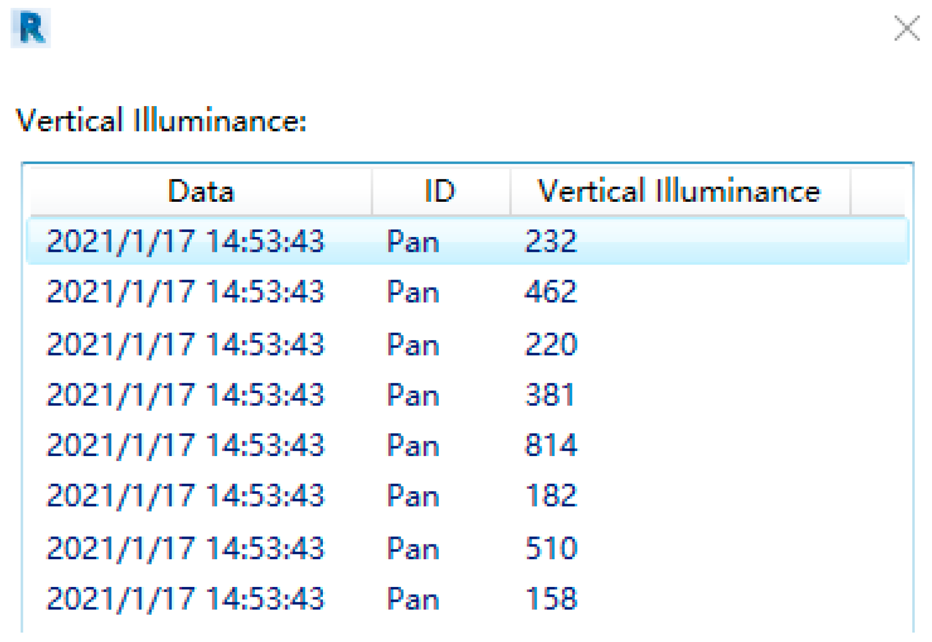
The personalized visual model was verified by a virtual room, considered as a case study. To confirm the reliability of the model, the environmental data were collected and imported into the BIM plug-in. The BIM plug-in was programmed by RF to predict appropriate vertical illuminance toward specific participants. The same participant was invited to assess the vertical illuminance calculated by the plug-in, and the result was confirmed to improve the participant’s comfort with the overall indoor office environment. Meanwhile, it can also save building energy consumption during operation and maintenance, making the building more in line with the concept of sustainable development.

The research in this paper has the following deficiencies: 1. This paper only uses four types of machine learning algorithms but does not find the best algorithm to predict indoor light illuminance in all machine learning methods; 2. The experimental data were collected in a month for each participant and ignored the influence of long-term visual satisfaction. 3. We divided visual perception into three parts (dim, comfort, bright) to assess accurately, but it may not reflect the feelings of individuals in detail.

Future research could focus on other machine learning algorithms and compare the performance with RF. Based on the algorithm, an intelligent control system of lighting equipment can be designed to adjust lighting automatically. In addition, the parameters about the interpersonal relationship could be added into the model because staff need to cooperate and communicate with others frequently. In other words, staff may change their positions in the open office.

References

1. Shaikh, P.H.; Nor, N.B.M.; Nallagownden, P.; Elamvazuthi, I.; Ibrahim, T. Robust stochastic control model for energy and comfort management of buildings. Aust. J. Basic Appl. Sci. 2013, 7, 137–144. [Google Scholar]
2. Bellia, L.; Fragliasso, F.; Pedace, A. Lighting control systems: Factors affecting energy savings’ evaluation. Energy Procedia 2015, 78, 2645–2650. [Google Scholar] [CrossRef] [Green Version]
3. China Building Energy Consumption Annual Report 2020. J. BEE 2020, 49, 1–6.
4. Pervez, P.H. Building energy management through a distributed fuzzy inference system. Int. J. Eng. Technol. 2013, 5, 3236–3242. [Google Scholar]
5. Xiong, J.; Tzempelikos, A.; Bilionis, I.; Awalgaonkar, N.M.; Lee, S.; Konstantzos, L.; AmirSadeghi, S.; Karava, P. Inferring personalized visual satisfaction profiles in daylit offices from comparative preferences using a bayesian approach. Build. Environ. 2018, 138, 74–88. [Google Scholar] [CrossRef]
6. Frontczak, M.; Wargocki, P. Literature survey on how different factors influence human comfort in indoor environments. Build. Environ. 2011, 46, 922–937. [Google Scholar] [CrossRef]
7. Kandasamy, N.K.; Karunagaran, G.; Spanos, C.; Tseng, K.J.; Soong, B.-H. Smart lighting system using ann-imc for personalized lighting control and daylight harvesting. Build. Environ. 2018, 139, 170–180. [Google Scholar] [CrossRef] [Green Version]
8. Veitch, J.A.; Charles, K.E.; Farley, K.M.J.; Newsham, G.R. A model of satisfaction with open-plan office conditions: COPE field findings. J. Environ. Psychol. 2007, 27, 177–189. [Google Scholar] [CrossRef] [Green Version]
9. Boyce, P.; Veitch, J.; Newsham, G.; Myer, M.; Hunter, C. Lighting quality and office work: Two field simulation experiments. Light. Res. Technol. 2006, 38, 191–223. [Google Scholar] [CrossRef] [Green Version]
10. Veitch, J.; Newsham, G.; Boyce, P.; Jones, C. Lighting appraisal, well-being, and performance in open-plan offices: A linked mechanisms approach. Light. Res. Technol. 2008, 40, 133–151. [Google Scholar] [CrossRef] [Green Version]
11. Suk, J.Y.; Schiler, M.; Kensek, K. Development of new daylight glare analysis methodology using absolute glare factor and relative glare factor. Energy Build. 2013, 64, 113–122. [Google Scholar] [CrossRef]
12. Goovaerts, C.; Descamps, F.; Jacobs, V.A. Shading control strategy to avoid visual discomfort by using a low-cost camera: A field study of two cases. Build. Environ. 2017, 125, 26–38. [Google Scholar] [CrossRef]
13. Zhang, Y.G.; Zhong, Y.W.; Gong, Y.D.; Zheng, L.R. The Optimization of Visual Comfort and Energy Consumption Induced by Natural Light Based on PSO. Sustainability 2019, 11, 49. [Google Scholar] [CrossRef] [Green Version]
14. Van Den Wymelenberg, K.G. Visual comfort, discomfort glare and occupant fenestration control: Developing a research agenda. Leukos 2014, 10, 207–221. [Google Scholar] [CrossRef]
15. Kent, M.G.; Altomonte, S.; Wilson, R.; Tregenza, P.R. Temporal effects on glare response from daylight. Build. Environ. 2017, 113, 49–64. [Google Scholar] [CrossRef]
16. Oh, M.H.; Lee, K.H.; Yoon, J.H. Automated control strategies of inside slat-type blind considering visual comfort and building energy performance. Energy Build. 2012, 55, 728–737. [Google Scholar] [CrossRef]
17. Yun, G.Y.; Yoon, K.C.; Kim, K.S. The influence of shading control strategies on the visual comfort and energy demand of office buildings. Energy Build. 2014, 84, 70–85. [Google Scholar] [CrossRef]
18. Konstantzos, I.; Tzempelikos, A.; Chan, Y.-C. Experimental and simulation analysis of daylight glare probability in offices with dynamic window shades. Build. Environ. 2015, 87, 244–254. [Google Scholar] [CrossRef]
19. Park, J.Y.; Dougherty, T.; Fritz, H.; Nagy, Z. Lightlearn: An adaptive and occupant centered controller for lighting based on reinforcement learning. Build. Environ. 2019, 147, 397–414. [Google Scholar] [CrossRef]
20. de Bakker, C.; Aries, M.; Kort, H.; Rosemann, A. Occupancy-based lighting control in open-plan office spaces: A state-of-the-art review. Build. Environ. 2017, 112, 308–321. [Google Scholar] [CrossRef]
21. Lee, S.; Bilionis, L.; Karava, P.; Tzempelikos, A. A Bayesian approach for probabilistic classification and inference of occupant thermal preferences in office buildings. Build. Environ. 2017, 118, 323–343. [Google Scholar] [CrossRef] [Green Version]
22. Karlsen, L.; Heiselberg, P.; Bryn, I.; Johra, H. Verification of simple illuminance-based measures for indication of discomfort glare from windows. Build. Environ. 2015, 92, 615–626. [Google Scholar] [CrossRef]
23. Konis, K. Predicting visual comfort in side-lit open-plan core zones: Results of a field study pairing high dynamic range images with subjective responses. Energy Build. 2014, 77, 67–79. [Google Scholar] [CrossRef] [Green Version]
24. Boubekri, M.; Boyer, L. Effect of window size and sunlight presence on glare. Light. Res. Technol. 1992, 24, 69–74. [Google Scholar] [CrossRef]
25. Jakubiec, J.A.; Reinhart, C.F. The “adaptive zone” –a concept for assessing discomfort glare throughout daylit spaces. Light. Res. Technol. 2012, 44, 149–170. [Google Scholar] [CrossRef]
26. Hirning, M.; Isoardi, G.; Cowling, I. Discomfort glare in open plan green buildings. Energy Build. 2014, 70, 427–440. [Google Scholar] [CrossRef] [Green Version]
27. van den Wymelenberg, K.; Inanici, M. A critical investigation of common lighting design metrics for predicting human visual comfort in offices with daylight. Leukos 2014, 10, 145–164. [Google Scholar] [CrossRef]
28. O’Brien, W.; Gunay, H.B. The contextual factors contributing to occupants’ adaptive comfort behaviors in offices—a review and proposed modeling framework. Build. Environ. 2014, 77, 77–87. [Google Scholar] [CrossRef]
29. Kar, P.; Shareef, A.; Kumar, A.; Harn, K.T.; Kalluri, B.; Panda, S.K. Revicee: A recommendation based approach for personalized control visual comfort & energy efficiency in buildings. Build. Environ. 2019, 152, 135–144. [Google Scholar]
30. Jakubiec, J.A.; Reinhart, C.F. A concept for predicting occupants’ long term visual comfort within daylit spaces. Leukos 2016, 12, 185–202. [Google Scholar] [CrossRef]
31. Aries, M.B.C.; Eitch, J.A.V.; Newsham, G.R. Windows, view, and office characteristics predict physical and psychological discomfort. J. Environ. Psychol. 2010, 30, 533–541. [Google Scholar] [CrossRef]
32. Leaman, A.; Thomas, L.; Andenberg, M.V. “Green” buildings: What Australian building users are saying. Ecolibrium 2007, 6, 22–30. [Google Scholar]
33. Yu, J.; Yang, C.; Tian, L. Low-energy envelope design of residential building in hot summer and cold winter zone in China. Energy Build. 2008, 40, 1536–1546. [Google Scholar] [CrossRef]
34. Littlefair, P.; Ortiz, J.; Bhaumik, C.D. A simulation of solar shading control on UK office energy use. Build. Res. Inf. 2010, 38, 638–646. [Google Scholar] [CrossRef]
35. Nielsen, M.V.; Svendsen, S.; Jensen, L.B. Quantifying the potential of automated dynamic solar shading in office buildings through integrated simulations of energy and daylight. Sol. Energy 2011, 85, 57–68. [Google Scholar] [CrossRef]
36. Palmero-Marrero, A.I.; Oliveira, A.C. Effect of louver shading devices on building energy requirements. Appl. Energy 2009, 87, 2040–2049. [Google Scholar] [CrossRef]
37. Li, D.Y.; Liu, C.Y.; Gan, W.Y. A new cognitive model: Cloud model. Intell. Syst. 2009, 24, 357–375. [Google Scholar] [CrossRef]
38. Li, J.; Fang, H.; Song, W. Modified failure mode and effects analysis under uncertainty: A rough cloud theory-based approach. Appl. Soft Comput. 2019, 78, 195–208. [Google Scholar] [CrossRef]
39. Huang, G.; Xiao, L. Failure mode and effect analysis: An interval-valued intuitionistic fuzzy cloud theory-based method. Appl. Soft Comput. 2021, 98, 106834. [Google Scholar] [CrossRef]
40. Safari, H.; Faraji, Z.; Majidian, S. Identifying and evaluating enterprise architecture risks using FMEA and fuzzy VIKOR. J. Intell. 2016, 27, 475–486. [Google Scholar] [CrossRef]
41. Huang, G.; Xiao, L.; Zhang, W.; Li, J.; Zhang, G.; Ran, Y. An improving approach for failure mode and effect analysis under uncertainty environment: A case study of critical function component. Qual. Reliab. Eng. Int. 2020, 36, 2119–2145. [Google Scholar] [CrossRef]
42. Sałabun, W.; Watróbski, J.; Shekhovtsov, A. Are MCDA Methods Benchmarkable? A Comparative Study of TOPSIS, VIKOR, COPRAS, and PROMETHEE II Methods. Symmetry 2020, 12, 1549. [Google Scholar] [CrossRef]
43. Shekhovtsov, A.; Sałabun, W. A comparative case study of the VIKOR and TOPSIS rankings similarity. J. Proc. 2020, 9, 3730–3740. [Google Scholar] [CrossRef]
44. Ahdani, B.V.; Salimi, M.; Charkhchian, M. A new FMEA method by integrating fuzzy belief structure and TOPSIS to improve risk evaluation process. Adv. Manuf. Technol. 2015, 77, 357–368. [Google Scholar] [CrossRef]
45. Liu, H.C.; Wang, L.E.; Li, Z.W.; Hu, Y.P. Improving Risk Evaluation in FMEA With Cloud Model and Hierarchical TOPSIS Method. IEEE Trans. Fuzzy Syst. 2019, 27, 84–95. [Google Scholar] [CrossRef]
46. Carlucci, S.; Causone, F.; de Rosa, F.; Pagliano, L. A review of indices for assessing visual comfort with a view to their use in optimization processes to support building integrated design. Renew. Sustain. Energy Rev. 2015, 47, 1016–1033. [Google Scholar] [CrossRef] [Green Version]
47. Leccese, F.; Salvadori, G.; Rocca, M.; Buratti, C.; Belloni, E. A method to assess lighting quality in educational rooms using analytic hierarchy process. Build. Environ. 2020, 168, 106501. [Google Scholar] [CrossRef]
48. Kim, W.; Kim, J.T. The Scope of the glare light source of the window with non-uniform luminance distribution. Indoor Built Environ. 2011, 20, 54–64. [Google Scholar] [CrossRef]
49. Bian, Y.; Dai, Q.; Ma, Y.; Liu, L. Variable set points of glare control strategy for side-lit spaces: Daylight glare tolerance by time of day. Sol. Energy 2020, 201, 268–278. [Google Scholar] [CrossRef]
50. Nabil, A.; Mardaljevic, J. Useful daylight illuminance: A new paradigm for assessing daylight in buildings. Light. Res. Technol. 2005, 37, 41–59. [Google Scholar] [CrossRef]
51. Chauvel, P.; Collins, J.B.; Dogniaux, R.; Longmore, J. Glare from windows: Current views of the problem. Light. Res. Technol. 1982, 14, 31–46. [Google Scholar] [CrossRef]
52. Einhorn, H.D. Unified glare rating (UGR): Merits and application to multiple sources. Light. Res. Technol. 1998, 30, 89–93. [Google Scholar]
53. Linney, A. Maximum Luminances and Luminance Ratios and Their Impact on Users’ Discomfort Glare Perception and Productivity in Daylit Offices. Master's Thesis, Victoria University of Wellington, Wellington, New Zealand, 2008. [Google Scholar]
54. Thornton, W.A. Color-discrimination index. J. Opt. Soc. Am. 1972, 62, 191. [Google Scholar] [CrossRef]
55. Davis, W.; Ohno, Y. Color quality scale. Opt. Eng. 2010, 49, 033602. [Google Scholar] [CrossRef] [Green Version]
56. Christoffersen, J.; Johnsen, K. Windows and daylight. A post-occupancy evaluation of Danish offices. In Proceedings of the in Lighting, CIBSE/ILE Joint Conference, York, UK, 9–11 July 2000; pp. 112–120. [Google Scholar]
57. Nazzal, A. A new evaluation method for daylight discomfort glare. Int. J. Ind. Ergon. 2005, 35, 295–306. [Google Scholar] [CrossRef]
58. Liu, Q.; Huang, Z.; Li, Z.; Pointer, M.R.; Zhang, G.; Liu, Z.; Gong, H.; Hou, Z. A Field Study of the Impact of Indoor Lighting on Visual Perception and Cognitive Performance in Classroom. Appl. Sci. 2020, 10, 21. [Google Scholar] [CrossRef]
59. Cuttle, C. Towards the third stage of the lighting profession. Light. Res. Technol. 2010, 42, 73–93. [Google Scholar] [CrossRef]
60. Kim, J.; Zhou, Y.; Schiavon, S.; Raftery, P.; Brager, G. Personal comfort models: Predicting individuals’ thermal preference using occupant heating and cooling behavior and machine learning. Build. Environ. 2018, 129, 96–106. [Google Scholar] [CrossRef] [Green Version]
61. Langevin, J.; Wen, J.; Gurian, P.L. Modeling thermal comfort holistically: Bayesian estimation of thermal sensation, acceptability, and preference distributions for office building occupants. Build. Environ. 2013, 69, 206–226. [Google Scholar] [CrossRef]
62. Meir, I.A.; Pearlmutter, D.; Etzion, Y. On the microclimatic behavior of two semienclosed attached courtyards in a hot dry region. Build. Environ. 1995, 30, 563–572. [Google Scholar] [CrossRef]
63. AlShaaby, A.; Aljamaan1, H.; Alshayeb, M. Bad Smell Detection Using Machine Learning Techniques: A Systematic Literature Review. Arab. J. Sci. Eng. 2020, 45, 2341–2369. [Google Scholar] [CrossRef]
64. Lu, H.F.; Ma, X.; Huang, K.; Azimi, M. Carbon trading volume and price forecasting in China using multiple machine learning models. J. Clean. Prod. 2019, 249, 119386. [Google Scholar] [CrossRef]
65. Zhang, Y.; Haghani, A. Agradient boosting method to improve travel time prediction. Transp. Res. Part C 2015, 58, 308–324. [Google Scholar] [CrossRef]
66. Kundu, S.; Sarker, G. An efficient integrator based on template matching technique for person authentication using different biometrics. Indian J. Sci. Technol. 2016, 9, 42. [Google Scholar] [CrossRef] [Green Version]
67. Majnik, M.; Bosnić, Z. ROC analysis of classifiers in machine learning: A survey. Intell. Data Anal. 2013, 17, 531–558. [Google Scholar] [CrossRef]
68. Stone, M. Cross-validatory choice and assessment of statistical predictions. J. R. Stat. Soc. Ser. B Methodol. 1974, 36, 111–113. [Google Scholar] [CrossRef]
69. Konstantzos, J.; Tzempelikos, A. Daylight glare evaluation with the sun in the field of view through window shades. Build. Environ. 2017, 113, 65–77. [Google Scholar] [CrossRef]
Figure 1. The experiment site.
Sustainability 13 07602 g001
Figure 2. The basic procedure of RF.
Sustainability 13 07602 g002
Figure 3. Relationship between learner numbers and OOB error.
Sustainability 13 07602 g003
Figure 4. One of predictive performance of personal comfort models and prediction accuracy is expressed as the average of all cross-validated AUCs respectively. (a) is RF; (b) is CTree; (c) is KSVM; (d) is GMM.
Sustainability 13 07602 g004
Figure 5. The confusion matrix of four machine learning methods. (a) is CTree; (b) is RF; (c) is GMM; (d) is KSVM.
Sustainability 13 07602 g005
Figure 6. Interface of individual visual comfort plug-in selection.
Sustainability 13 07602 g006
Figure 7. Selecting the plug-in.
Sustainability 13 07602 g007
Figure 8. Plug-in parameters setting.
Sustainability 13 07602 g008
Figure 9. Individual vertical illuminance calculation results.
Sustainability 13 07602 g009