Article

Unemployment Rates Forecasting with Grey-Based Models in the Post-COVID-19 Period: A Case Study from Vietnam

1
Department of Business Management, National Taipei University of Technology, Taipei 10608, Taiwan
2
Faculty of Business, FPT University, Hanoi 100000, Vietnam
3
Department of Economics, Faculty of Social Sciences and Humanities, Konya Food and Agriculture University, Konya 42080, Turkey
4
Department of Urban Industrial Management and Marketing, University of Taipei, Taipei 11153, Taiwan
*
Author to whom correspondence should be addressed.
Sustainability 2021, 13(14), 7879; https://doi.org/10.3390/su13147879
Submission received: 2 June 2021 / Revised: 10 July 2021 / Accepted: 12 July 2021 / Published: 14 July 2021

Abstract

:
The Coronavirus (COVID-19) pandemic has had a significant impact on most countries’ social and economic perspectives worldwide. Unemployment has become a vital challenge for policymakers as a result of COVID-19′s negative impact. Because of the nonstationary and nonlinear nature of the dataset, researchers applied various time series models to forecast the unemployment rate. This study aims to ensure a better forecasting approach for predicting the unemployment rates with an uncertainty of insufficient knowledge and tiny data throughout Vietnam. The study proposes the Grey theory system-based GM (1,1), the Grey Verhulst Model (GVM), and the Autoregressive Integrated Moving Average (ARIMA) model that can more precisely predict unemployment rates. The model’s applications are shown using the Vietnamese unemployment rate at six different rural and urban areas with data sets from 2014–2019. The results indicate that the lower Mean Average Percentage Error (MAPE) values obtained with the GM (1,1) model at all regions for rural and urban areas (excluding Highlands Region in urban area) are extremely encouraging in comparison to other traditional methods. The accurate level of the ARIMA and GVM models follows the GM (1,1) model. The findings of this study show that the effects of the modeling assist policymakers in shaping future labor and economic policies. Furthermore, this study can contribute to the unemployment literature, providing future research directions in the unemployment problems.

1. Introduction

The principal macroeconomic variable is unemployment, and public policies demand knowledge of how this variable will evolve. Current global issues such as the Great Recession of 2008, the Eurozone economic crisis, and the COVID-19 epidemic all happened despite significant disparities across nations [1,2].
The US Bureau of Labor Statistics announced that total nonfarm employment decreased by 140,000 in December, but the unemployment was unchanged at 6.7%. The mass unemployment is a consequence of the recent increase in COVID-19 cases and containment efforts. Jobs lost in leisure and hospitality and private education were slightly offset by growth in technology and business services, retail commerce, and construction. According to Eurostat’s official statistics, the Eurozone’s seasonally adjusted unemployment rate decreased to 8.3% in November 2020, down from 8.4 percent the previous month and getting closer to the more than two-year high of 8.7% set in July. Spain (16.4%), Italy (8.9%), and France (8.8%) had the highest unemployment rates, while the Netherlands (4.0%) and Germany had the lowest (4.5%).
According to a July 2020 report by the Vietnamese General Statistics Office (GSO), 30.8 million individuals across the whole country were directly and seriously harmed by COVID-19. The service sector was hardest hit by COVID-19, accounting for 72% of affected employees, followed by manufacturing and construction at 67.8%; agriculture, forestry, and fishery accounted for 25.1% of affected workers. The pandemic’s effects resulted in Vietnam’s highest unemployment rate in ten years, with low-skilled workers bearing a disproportionate share of the burden. Unemployment is a socioeconomic issue that is influenced by a myriad of cause-and-effect elements. As a result, a substantial study on the interaction of economic and social variables affecting unemployment is crucial [3]. Following the challenges that have arisen due to the current economic crisis and increased rural–urban migration, unemployment is a significant indication for the general population, the Vietnamese government, and scholars [4].
In this context, one of the primary policy objectives of government macroeconomic management is to keep unemployment low. A more precise unemployment rate estimate is thus needed, which adds to the upward pressure on the unemployment rate.
To the authors’ knowledge, examining determinants of unemployment problems and forecasting unemployment rates have been involved in various studies; however, the circumstances in Vietnam have rarely been reflected. Therefore, the objectives of this study are to (i) describe the unemployment rates in different regions of Vietnam using suitable models, (ii) perform future forecasting for these models, and (iii) propose some policy recommendations for these regions.
To fill this empirical research gap, the authors conducted novel and timeless research on this issue for a problematic paradigm in Vietnam. Three forecasting time series techniques of GM (1,1), GVM, and ARIMA model were employed in Vietnamese unemployment rates at six different regions for rural and urban areas. In this study, the period 2014 to 2019 was employed as the training dataset for estimating reliable predicting results using MAPE values. Then, the prediction for the unemployment rate for the following five years, 2020–2025, was provided. These forecasting techniques are compared in order to obtain a better understanding of their different strengths and shortcomings.
The significant contribution of this paper is to provide the most exact forecasting approach possible for predicting the unemployment rate given the uncertainty of insufficient knowledge and tiny data.
The remainder of this study proceeds as follows: In Section 2, a quick overview of relevant studies is provided. Section 3 summarizes the empirical data and proposed methods utilized in the analysis. Section 4 presents the findings of the forecasting models that were estimated. Finally, Section 5 concludes with conclusions and recommendations.

2. Literature Review

Economic development, social development, and environmental protection are three pillars of the concept of sustainability. Unemployment and economic growth are inextricably linked in both emerging and established economies worldwide. In this perspective, the relationship between unemployment and political stability, in which a particular political environment preserves a country’s tolerable unemployment, may aid in developing a long-term economic, social, and political framework. Numerous previous research has demonstrated the connections between unemployment, gross domestic product (GDP), foreign direct investment (FDI), and social security in a variety of contexts [5,6,7,8,9].
Various research has been performed on the estimation of unemployment rates. Researchers employ both qualitative and quantitative forecasting strategies, which can be classified into two types of predictive methods: univariate and multivariate models such as time series forecasting model [10,11,12], regression model [13,14,15,16], artificial neural networks [17,18,19,20,21], and so on.
Adam et al. [22] provided a quantitative econometric approach to assess the relationship between effective economic and rational policy, nominal wage inflation, and unemployment. Their findings revealed that lowering the unemployment rate could boost the living and economic growth in Sudan.
On the one hand, Abouelfarag and Qutb [23] investigated the correlation between government expenditure and unemployment in Egypt between 1980 and 2017 through an empirical examination. The empirical findings of this study established that an increase in government expenditure results in an increase in unemployment over the long run. Misra and Singh [24] devised a nonlinear mathematical model for the problem of unemployment from an earlier stage. The stability theory for differential equations was used to examine the number of unemployed, those working temporarily, and those working full-time.
As studied by Raneah et al. [25], a mathematical model was developed utilizing the unemployment rate and the number of jobless and skilled unemployed persons. Their data demonstrated a strong correlation between educational programs and real-world unemployment rates. As explored by Shimer [26], microeconomic data was applied to measure the unemployment probability. His results contradicted the conventional wisdom that guided the development of the labor market’s macroeconomic models since 1990.
There is substantial literature on macroeconomic modeling and forecasting using historical data from univariate or multivariate time series. Historically, unemployment rates, similar to any other macroeconomic variable, have been analyzed using econometric models, frequently based on stationary time series. These models include trend analysis and exponential smoothing (ARIMA), as well as the simple Ordinary Least Squares (OLS) techniques, the Generalized Autoregressive Conditional Heteroskedasticity (GARCH) models, and neural networks [27,28,29].
The ARIMA model was used by Claveria [30] to examine unemployment rates in eight European Union countries between 2007 and 2017. Moreover, Ahmad et al. [31] used a hybrid ARIMA-SVM-ARNN prediction methodology to forecast unemployment rates for six selected European nations, notably France, Spain, Belgium, Turkey, Italy, and Germany.
Recently, Davidescu et al. [32] used a variety of forecasting models to estimate the Romanian unemployment rate for the period 2021–2022, including the seasonal model autoregressive integrated moving average (SARIMA), the self-exciting threshold autoregressive (SETAR), Holt–Winters, ETS (error, trend, seasonal), and NNAR (neural network autoregression).
Among them, Gil-Alana [33] used an exponential Bloomfield spectral model to analyze unemployment in the UK. As studied in other research, Autoregressive moving average (ARMA) models, which have been investigated in earlier studies, were used by Wong et al. [34] to assess and forecast Hong Kong’s economic indices from 1983 to 2002. Regarding a recent study of Naccarato et al. [35], the unemployment rate in Italy using ARIMA and Vector-Autoregressive Models (VAR) was analyzed by combining official and Google Trends data.
The forecasting models and their extensions have been applied in the real world to overcome the complexity and uncertainty [36,37,38,39]. Grey theory is primarily concerned with ambiguous system models in which there is inadequate information to perform system link analysis, model creation, predictions, and judgments. Grey system theory applies to the following application areas: grey generation, grey relational analysis, grey forecasting, grey decision making, and grey control. Grey forecasting is an essential and often utilized sort of forecasting [40]. When system information is insufficient, grey models can be applied to describe the behavior of a few outputs with little data [41,42].
As mentioned above, unemployment is affected by many uncertain factors such as economic, social, and political frameworks; therefore, unemployment forecasting can be a grey system problem. For unemployment time series prediction, it requires only four recent samples to derive reliable and acceptable prediction accuracy so that GM (1,1) is applied in this study. Furthermore, the Grey Verhulst model (GVM) has been widely used in many fields [43,44,45,46,47,48]. Therefore, this method can be suitable for predicting the unemployment rate.

3. Proposed Methods

To overcome the limitations of previous studies on the forecasting precision of unemployment rate, this study employs the GM (1,1) and GVM models for theoretical derivation and verification, followed by a comparison of the two proposed grey models with the ARIMA regression analysis model to determine the optimal model with the highest forecasting precision, the lowest MAPE, and fitness.

3.1. Grey Forecasting Model—GM (1,1)

Initially proposed by Deng [40], Grey theory is a truly multidisciplinary and genre-specific theory that deals with systems with little or no information. The grey theory typically works with weak, inaccurate, or unclear messages on systems analysis. The GM (1,1) is commonly applied to solve problems in an uncertain environment.
Step 1: Present x ( 0 ) as the original series of data with n observations:
g ( 0 ) = ( g ( 0 ) ( 1 ) , g ( 0 ) ( 2 ) ,   g ( 0 ) ( 3 ) , ,   g ( 0 ) ( n ) )
Step 2: Propose g ( 1 ) is the first-order Accumulated generating operator (1-AGO) from g ( 0 ) series:
g ( 1 ) = ( g ( 1 ) ( 1 ) ,   g ( 1 ) ( 2 ) ,   g ( 1 ) ( 3 ) , , g ( 1 ) ( n ) ) g ( 1 ) = ( Σ k = 1 1   g ( 0 ) k ,   Σ k = 1 2   g ( 0 ) k , , Σ k = 1 n g ( 0 ) ( k ) )
Step 3: Propose that GM (1,1) with grey differential equation and z ( 1 ) value is computed by using g ( 0 ) and g ( 1 ) series:
g ( 0 ) ( k ) + a z ( 1 ) ( k ) = b ,   k = 2 , 3 , ,   n z ( 1 ) = 0.5 g ( 1 ) ( k ) + 0.5 g ( 1 ) ( k 1 )
where k represents the time points, a is the development coefficient, and b is the grey control coefficient.
Step 4: The least-squares method is used to calculate a ^ coefficient in Equations (4)–(6):
a ^ = [ a b ] = ( B T B ) 1 B T Y N
B = [ z 1 ( 1 ) ( 2 ) 1 z 1 ( 1 ) ( 3 ) . . . z 1 ( 1 ) ( n ) 1 . . . 1 ] Y N   = [ g ( 0 ) ( 2 ) g ( 0 ) ( 3 ) . . . g ( 0 ) ( n ) ]
d g ( 1 ) d t + a g ( 1 ) = b
Step 5: The solution of the grey differential equation g ( 1 ) is utilized in Equation (7):
  g   ^ ( 1 ) ( k + 1 ) = [ g ( 0 ) ( 1 ) b a ] e a k + b a
Step 6: Forecast values of   g   ^ ( 0 ) ( k ) are obtained by Inverse-Accumulated generating operator (I-AGO) on   g   ^ ( 1 ) ( k + 1 ) :
  g   ^ ( 0 ) ( k ) =   g   ^ ( 1 ) ( k )   g   ^ ( 1 ) ( k 1 )   g   ^ ( 0 ) ( k ) = [ g ( 0 ) ( 1 ) b a ] e a ( k 1 ) ( 1 e a )
Step 7: Measure the efficiency of GM (1,1) by Mean Absolute Percentage Error (MAPE) values:
Δ ( k ) = | ε ( 0 ) k g ( 0 ) k |   100 % ,   k = 2 , 3 ,   ,   n ;   ε ( 0 ) k = g ( 0 ) k   g   ^ ( 0 ) k
The efficiencies of MAPE values are shown in Table 1.

3.2. Grey Verhulst Model (GVM)

Francois Verhulst proposed the Verhulst model in 1837. The grey Verhulst model is highly predictive of the data’s underlying process. The new predicted value is appended to the original sample sequence, and the sample sequence’s initial data point is deleted [44]. The GVM is presented in the following steps:
Step 1: Present g ( 0 ) to be the original time series and g ( 1 ) to be the raw time series,
g ( 0 ) = ( g ( 0 ) ( 1 ) , g ( 0 ) ( 2 ) ,   g ( 0 ) ( 3 ) , ,   g ( 0 ) ( n ) ) ; g ( 1 ) = ( g ( 1 ) ( 1 ) ,   g ( 1 ) ( 2 ) ,   g ( 1 ) ( 3 ) , , g ( 1 ) ( n ) ) Step 2: Propose that g ( 1 ) is the first-order Accumulated generating operator (1-AGO) from the g ( 0 ) series, increasing the z ( 1 ) series:
g ( 1 ) ( k ) = Σ i = 1 k g ( 0 ) ( i ) ,   k = 1 , 2 , ,   n
z ( 1 ) = ( z ( 1 ) ( 1 ) ,   z ( 1 ) ( 2 ) ,   z ( 1 ) ( 3 ) , , z ( 1 ) ( n ) )
Step 3: Propose the GVM with grey differential equation and z ( 1 ) value:
z ( 1 ) ( k ) = 1 2 ( g ( 1 ) ( k ) + g ( 1 ) ( k 1 ) ) , k = 2 , 3 , , n
Step 4: The least-squares method is used to calculate a ^ coefficient:
d g ( 1 ) d t + a g ( 1 ) = b ( g ( 1 ) ) 2
  g ( 0 ) ( k ) + a z ( 1 ) ( k ) = b ( z ( 1 ) ( k ) ) ( 2 )
In Equation (13), similar to GM (1,1), k is defined as the time dots, a is defined as the development coefficient, and b is defined as driver coefficient. Through Equations (10) and (13), the a ^ coefficient is obtained by using the least-squares method similar to GM (1,1):
a ^ = [ a b ] = ( B T B ) 1 B T Y N
B = [ z 1 ( 1 ) ( 2 ) ( z ( 1 ) ( 2 ) ) 2 z 1 ( 1 ) ( 3 ) . . . z 1 ( 1 ) ( n ) ( z ( 1 ) ( 3 ) ) 2 . . . ( z ( 1 ) ( n ) ) 2 ] Y N   = [ g ( 1 ) ( 2 ) g ( 1 ) ( 3 ) . . . g ( 1 ) ( n ) ]
Step 5: The solution of the GVM differential equation of g ( 1 ) (t) for k time, is obtained as follows:
  g   ^ ( 1 ) ( k + 1 ) = a g ( 0 ) ( 1 ) b g ( 0 ) ( 1 ) + ( a b g ( 0 ) ( 1 ) e a k
Step 6: Measure the efficiency of GM (1,1) by Mean Absolute Percentage Error (MAPE) values as follows:
Δ ( k ) = | ε ( 1 ) ( k ) | g ( 1 ) k ,   ε ( 1 ) k = g ( 1 ) k   g   ^ ( 1 ) ( k )

3.3. Autoregressive Integrated Moving Average Model (ARIMA)

An Autoregressive Integrated Moving Average (ARIMA) model was proposed by Box and Jenkins [49] as a combination of autoregression and a moving average model. This model is used to forecast time series data. The whole model is defined below:
y t λ = c + φ 1 y t 1 λ + + φ p y t p λ   + θ 1 ε t 1 + + θ q ε t q + ε t
where y t λ is the differenced series. On the right side, the equation includes both lagged values of y t and lagged errors (between ε t 1 and ε t q ). P shows the order of the autoregressive part, d is the differencing to achieve stationarity, and q is the order of moving average part at ARIMA(p,d,q) model. The ARIMA model can be written in backshift (B) notation as below:
( 1   φ 1 B φ p B p )   ( 1 B ) d y t λ   = c + ( 1 + θ 1 B + + θ q B q )   ε t
Using this notation [Equation (19)], we replaced t with t+1 to forecast future unemployment rates. Equation (20) shows the t+1th period of the forecasted value of unemployment rates as follows:
y t + 1 λ ^ =   ( 1 + φ 1 ^ )   y t λ ( φ 1 ^ φ 2 ^ )   y t 1 λ     ( φ p ^ ) y t p λ + θ 1 ^ ε t
The process continues with this method for all future periods. In this way, any number of point forecasts can be obtained up to replacing t with t + p times. The mean absolute percentage error (MAPE) obtained as a result of ARIMA is calculated by the Equation (21) to compare different methods as follows:
Δ t = | y λ t y ^ ( λ ) t y λ t |   100 % ,   t = 2 , 3 ,   ,   n

4. Results and Analyses

4.1. Data Collection and Description

This study was conducted to investigate the unemployment problems throughout Vietnam. The study area is examined based on two categories: rural and urban areas in six administrative regions (Red River Delta—RRD; Northern Midlands and Mountains—NMM; North Central Region—NCR; Highlands Region—HLR; Southeast Region—SER; Mekong River Delta—MRD). The data employed in this study is a set of secondary data about the unemployment rate from the years from 2014 to 2019, which is extracted from the database of the Vietnam General Office of Statistics (https://www.gso.gov.vn/, accessed on 30 July 2020).

4.2. Results from GM (1,1)

Table 2 and Table 3 compare the unemployment rate in rural and urban areas of Vietnam’s six administrative regions from 2014 to 2025. It is quite evident that the unemployment rate for urban areas would follow a downward trend until 2025 due to the industrialization and modernization process. By contrast, the rural unemployment rate might continue to rise because of the process’s impacts. It could be seen that the unemployment rate in the urban areas tends to be higher as opposed to that in rural areas. Specifically, the average forecasted unemployment rate in urban regions ranges between 2.5% and 3.5%, while the figures for rural areas are below 2%. The reason for this phenomenon is not explained by the population scale of each region since, according to Vietnam General Statistics Office, there were approximately 37,6 million rural laborers and about 18 million in urban regions as of 2019 (https://www.gso.gov.vn/ accessed on 30 July 2020). Because the population scale could not explain the higher unemployment rate in urban regions, Vietnamese experts have interpreted a rising demand for qualified laborers in big cities; with this demand comes stricter recruitment procedures and lower the chances for unqualified laborers.
Moreover, high-skilled laborers look for jobs that offer decent pay, and low-skilled workers do everything for their livelihood. Therefore, high-skilled laborers might suffer from frictional unemployment during the job-seeking period. In addition, reference data from the GSO indicated a downward trend for the RRD because the region now has the highest education level in Vietnam. In 2018, the proportions of secondary school, high school, and university graduates were estimated at 39% and 31.6%, respectively. Moreover, supporting the trend is an influx of Foreign Direct Investment (FDI) into the region. According to statistics from the Foreign Direct Investment Department of the Ministry of Planning and Investment, as of 2015, the number of newly registered investment projects was recorded at 606, amounting to USD 2.6 billion. In addition to that, capital-increasing projects accounted for about 62.5% of the region’s total FDI.
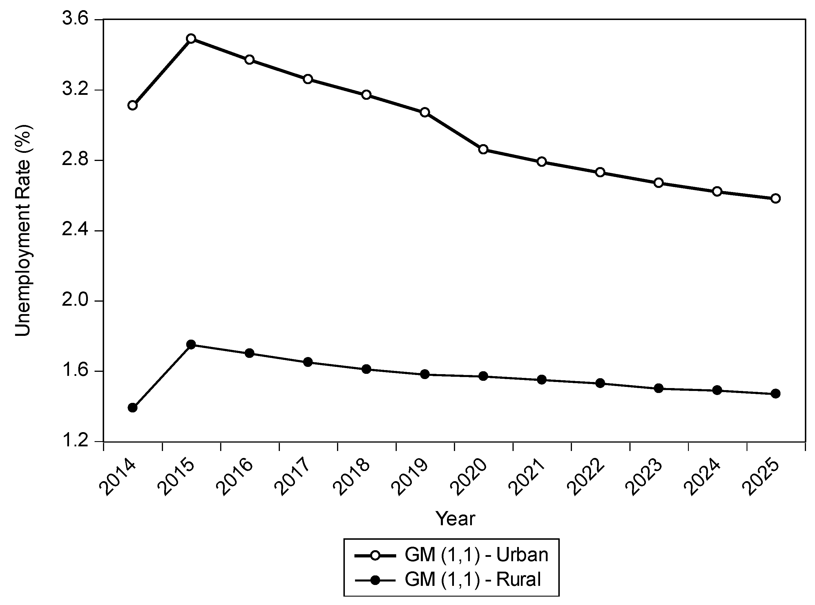
Moreover, the accumulated calculations specified the number of 5800 registered projects since the ‘Doi Moi’ policy; foreign investment projects in the Red River Delta made up 30% of the total projects in Vietnam, accounting for approximately 26% of the total amount of FDI in the country. The FDI data from a report in 2017 by the Foreign Direct Investment Department showed a significant increase in the number of new projects. It was estimated that in 2017, the Red River Delta had attracted nearly 7202 projects, which were worth USD 81.76 billion. According to GM (1,1) model, the average forecastings of unemployment rates in urban and rural areas are shown in Figure 1.
From Figure 1, it is seen that the forecasts of unemployment rates show a descending trend based on GM (1,1) model. Average forecasting of urban areas’ unemployment rates will reach above 2.5%. However, this rate decreases by approximately 1.5% in rural areas. In the context of GM (1,1) model predictions, the unemployment rates for each region will be evaluated between Figure 2, Figure 3, Figure 4, Figure 5, Figure 6, Figure 7, Figure 8, Figure 9, Figure 10, Figure 11, Figure 12 and Figure 13, separately.
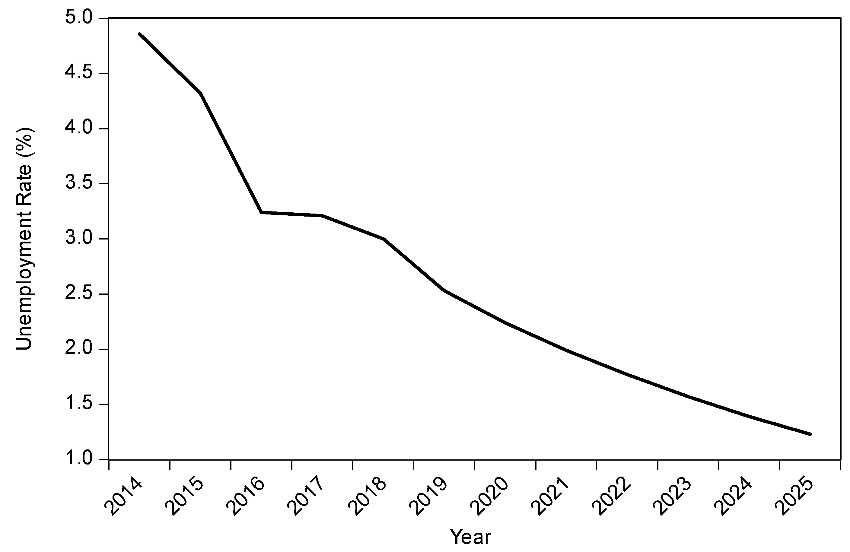
According to Figure 2, it is clear that the unemployment rate in the urban area of the Red River Delta region declined as time went on. The unemployment rate in that region was around 4.86%; then it decreased by 11.1% to 4.32% in the next year. After that, the unemployment rate declined significantly by 25% to around 3.24% in 2016. Since the sharp decline in 2016, in the following years, the unemployment rate maintained at around 3% in 2018. In the latest update, the unemployment rate in the region decreased to 2.53% in 2019. In addition, it is estimated that the Red River Delta’s urban area’s unemployment rate would continue to decrease in the following years, from 2.53% to 1.23% in 2025.
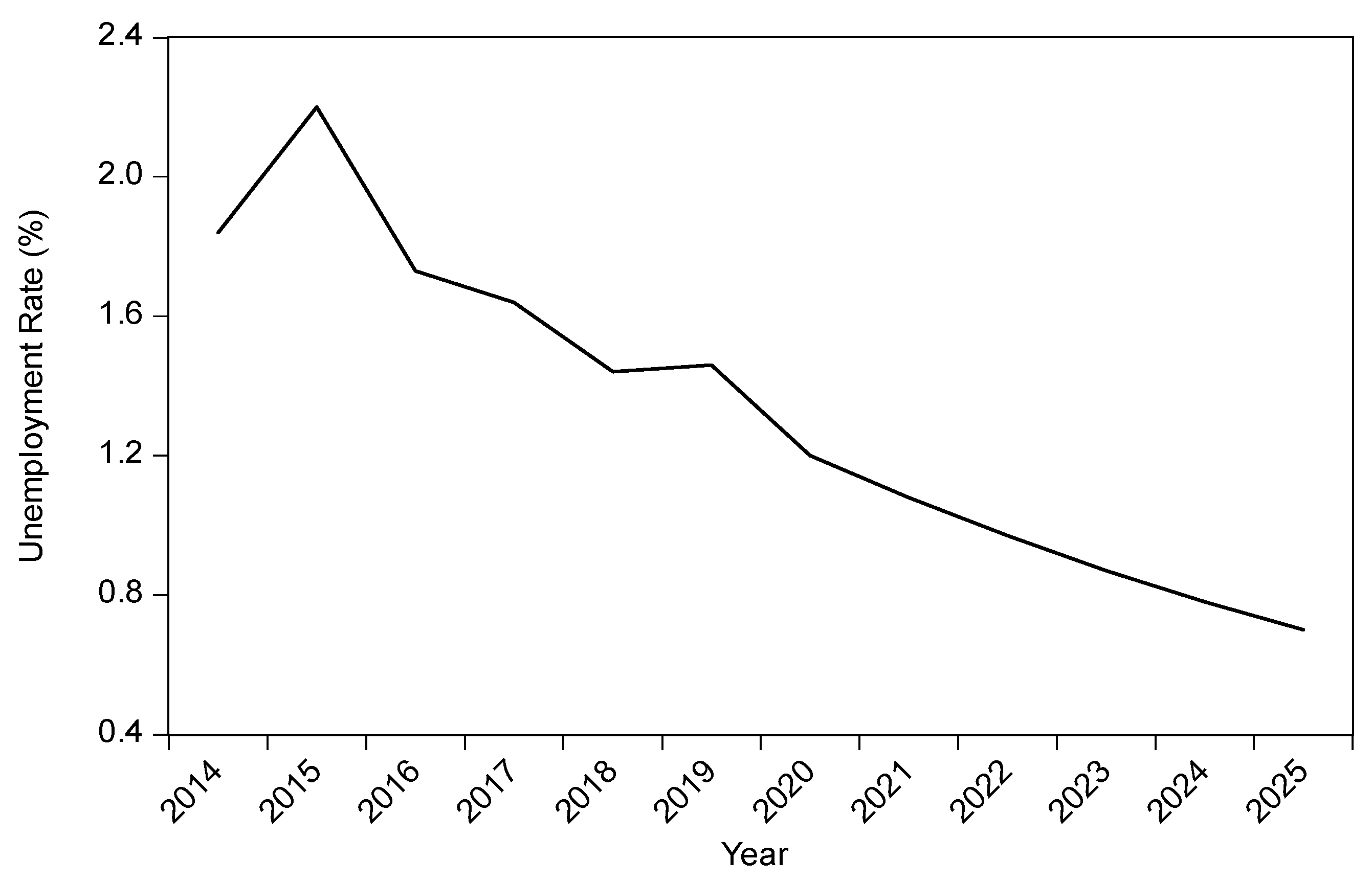
Regarding the unemployment rate in the Red River Delta’s rural area, as shown in Figure 3, the unemployment rate decreased for most of the period. On the one hand, there was only a sharp increase in the year 2015. In 2014, the number of unemployed in the total number of employed people was recorded at 1.84%. In 2015, the unemployment rate increased by approximately 20% to 2.2%, which declined by 21.4% to 1.73% in 2016. In the next three years, the unemployment rates were between 1.44% and 1.64%; it could continue this downward trend and decrease to 0.7% by 2025.
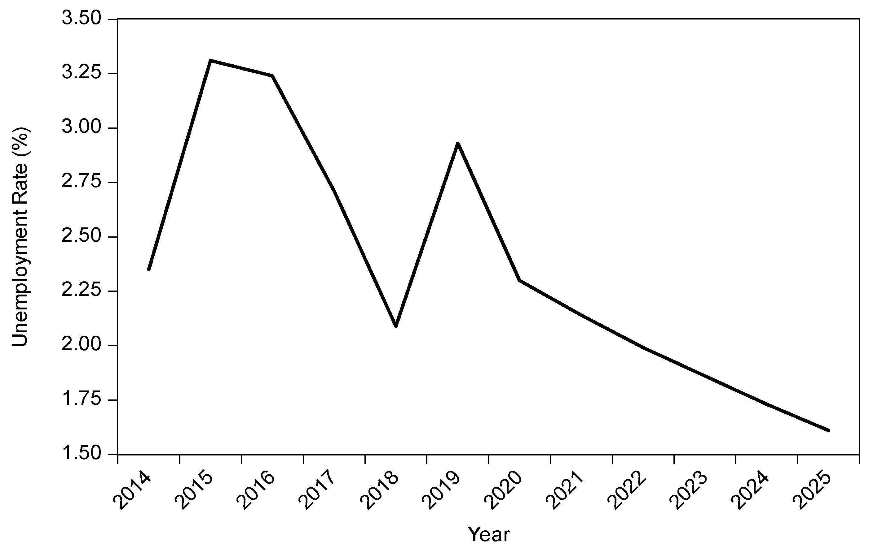
As shown in Figure 4, the urban unemployment rate in the Northern Midlands and Mountains was estimated at 2.4% in 2014. It then rose by 37.5% to 3.3% in 2015. However, the unemployment rate declined significantly to 2.09% in 2018, which was 22% lower than the rate for the year 2016. The year 2019 saw an increasing unemployment rate at 2.93%, up 38% from the previous year. In the next six years, the unemployment rate is estimated to continue a downward trend as it would decrease gradually from 2.9% to 1.6% in 2025.
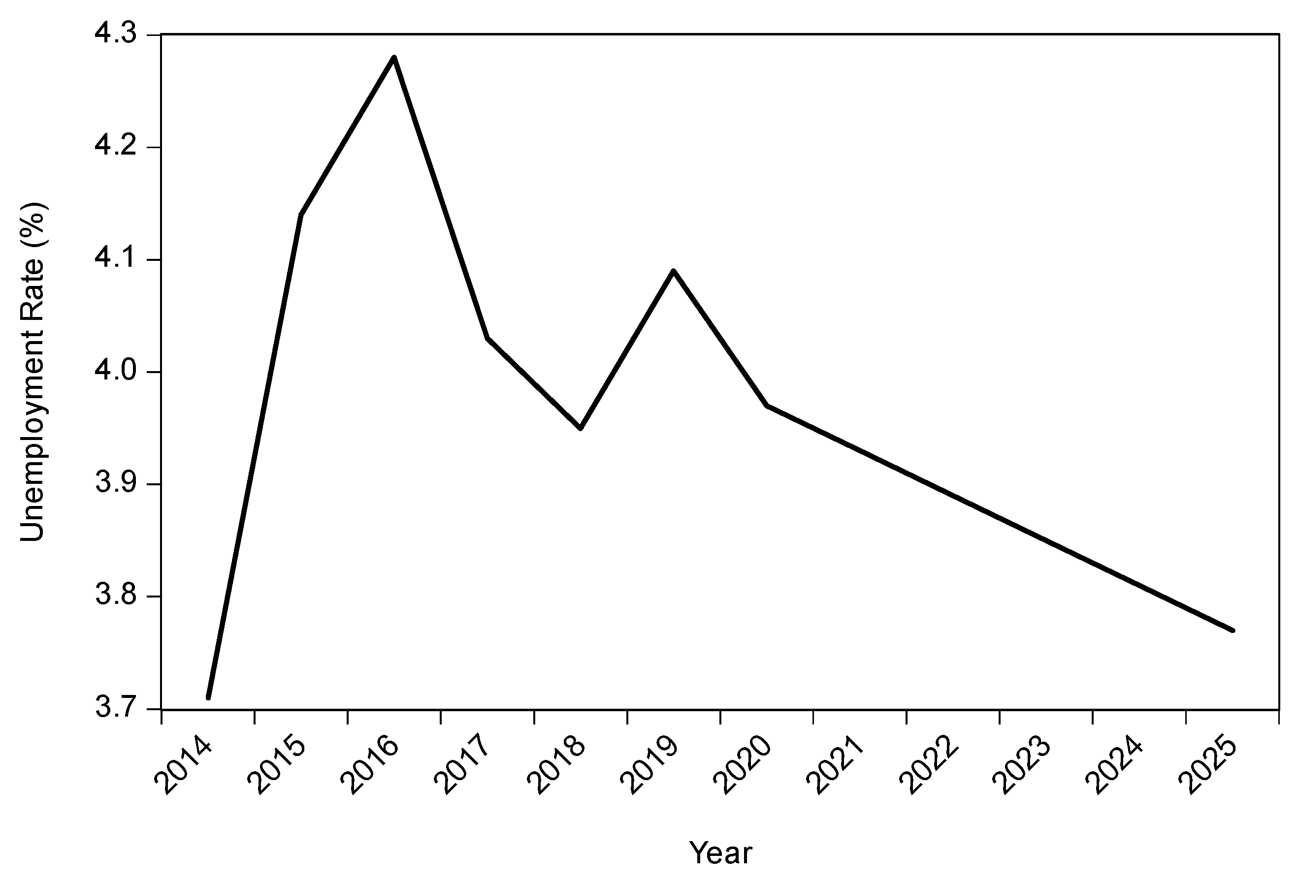
Figure 5 shows the unemployment rate for the rural area of the Northern Midlands and Mountains. It can be seen that the rural unemployment rate reached 0.85% in 2015, a tremendous increase from 2014, then it decreased to 0.78% in 2016. Following the downward trend, the rate decreased to 0.69% in 2017. There were increases in the rate of 0.85% in 2018 and 0.98% in 2019. Estimations for the period from 2020–2025 indicate that the unemployment rate would continue its downward trend as it could increase to about 1.17% by 2025. Figure 6 shows the unemployment rate for the urban area of the North Central region. The North Central region’s unemployment rate was quite volatile. Starting at 3.71% in 2014, it increased at the rate of 11.6% to 4.14% in 2015. In the following years, the urban unemployment rate fluctuated between 3.95% to 4.28%. The rate is then expected to decrease for the next six consecutive years to around 3.77% in 2025.
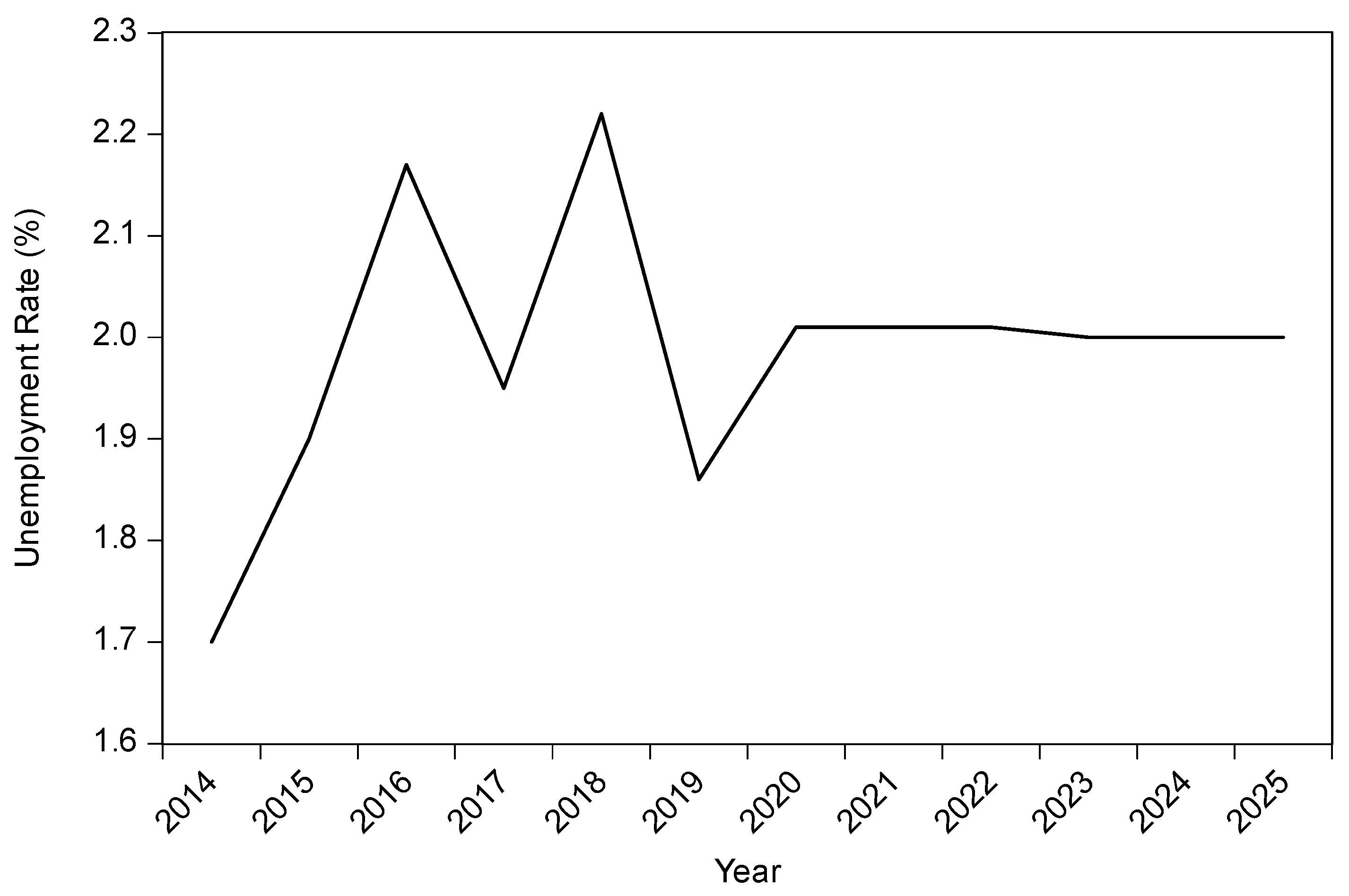
According to Figure 7, the unemployment rate increased continuously from around 12% to 14% in the first three years of the period. Nevertheless, it fluctuated around 2% in the next three years, and this trend is estimated to continue until 2025.
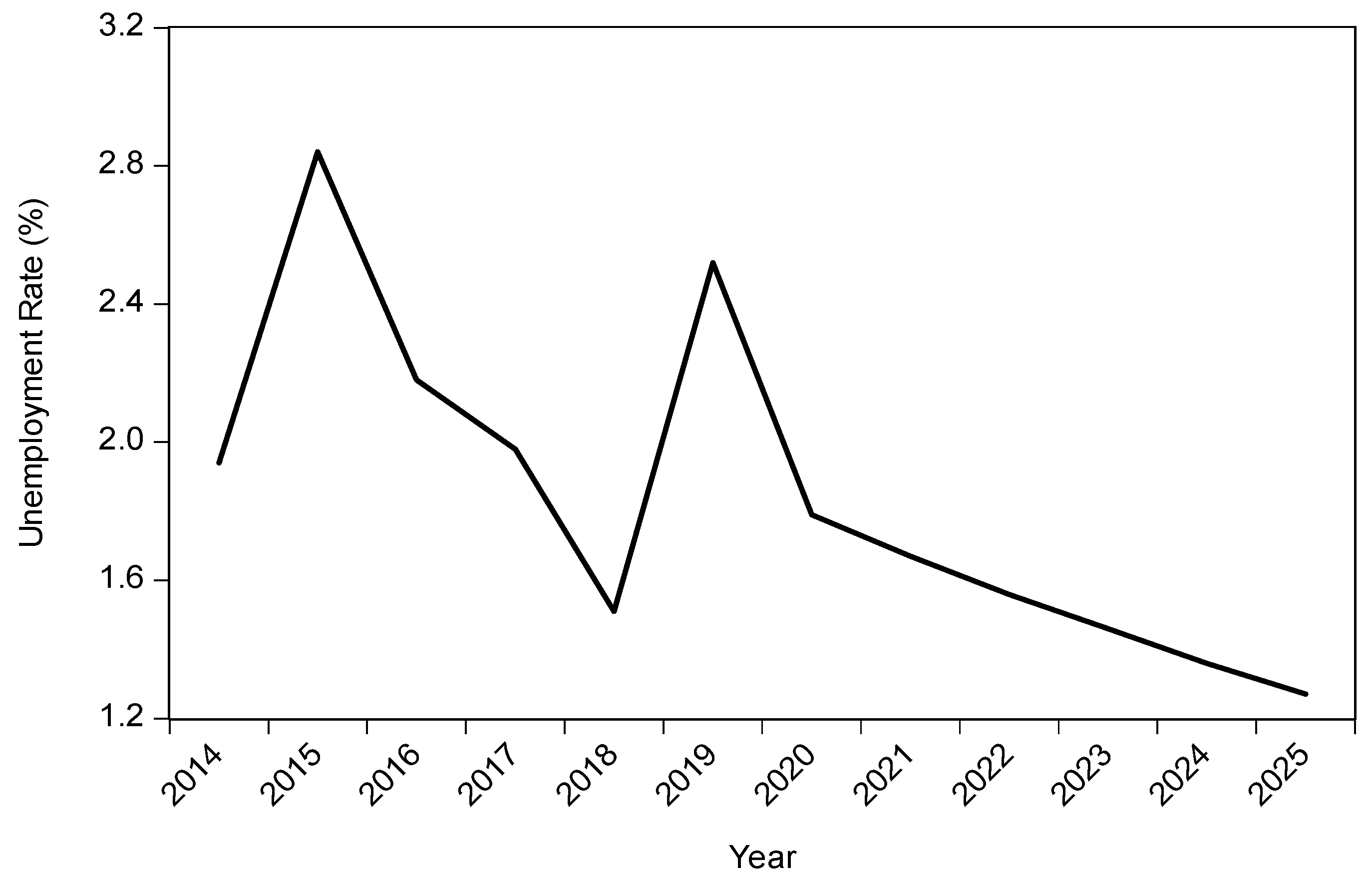
Concerning the percentage of the unemployed in the Highlands region’s urban area, it is pretty visible that the rate increased by nearly 50% from 1.94% in 2014 to 2.84% in 2015 (see Figure 8). After that, the rate experienced declines in 2016, 2017, and 2018 before witnessing a high rise in 2019. It is expected that the rate could continue its downward trend in the next six years as it might decrease to 1.27% in 2025.
Figure 9 shows the unemployment rate for the rural area of the Highlands. Starting at 0.93% in 2014, the unemployment rate in the rural area of the Highlands region decreased to 0.76% in 2015. The year 2017 was quite similar to that of 2015 as the rate decreased to 0.69% from 0.88% in 2016. Finally, in 2019, there was a slight increase in the rate, from 0.88% to 0.94%. In the next six years, the trend is expected to increase to 1.18% in 2025.
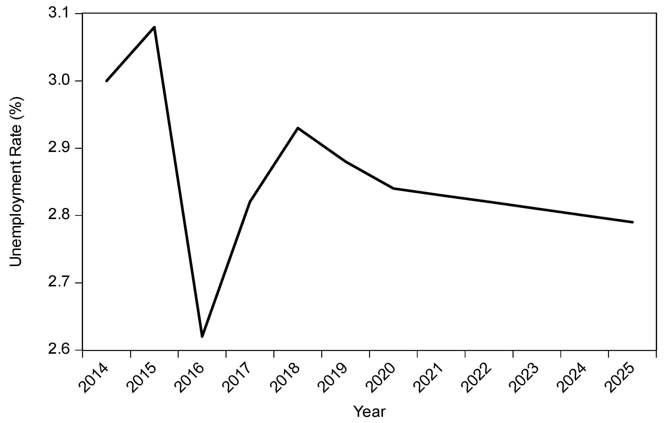
According to Figure 10, the average unemployment rate in the urban Southeast region during the period from 2014—2019 was about 2.88%, with the rate in 2015 being the highest, followed by the rates for the years 2014, 2018, 2019, 2017, and 2016. Then, in the following years, the unemployment rate for this region is expected to decline year after year to 2.79% in 2025.
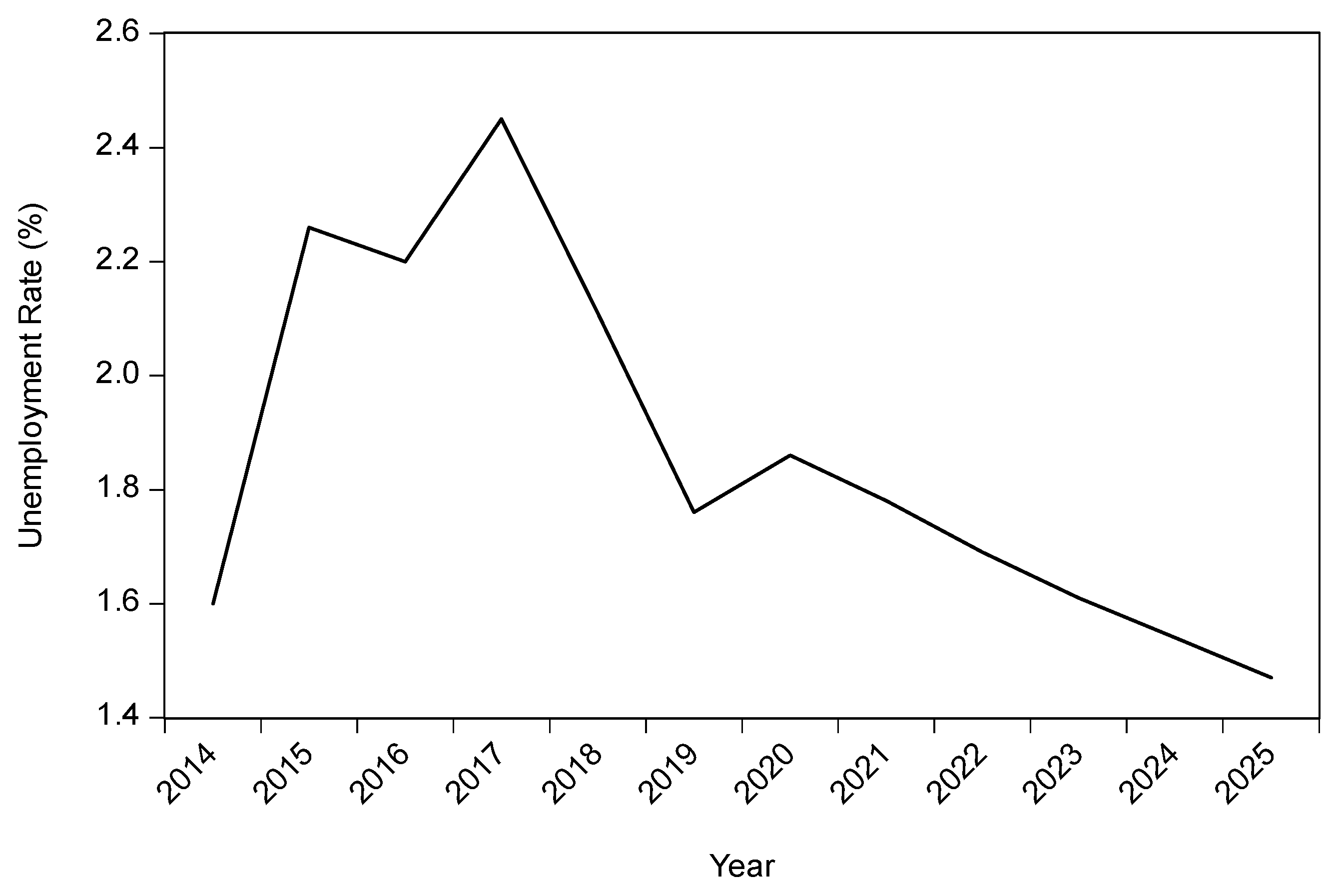
Figure 11 shows the unemployment rate for the rural area of the Southeast region. Between 2014 and 2019, the unemployment rate stood at 1.60% 2014. Then, there was a rise to 2.26% in 2015 before falling to 2.2% in the rural unemployment rate in the Southeast region in 2016. The rate then increased to 2.45% in 2017. From 2020 to 2025, the percentages for the unemployed in this region’s rural area are expected to decrease by 1.47%.
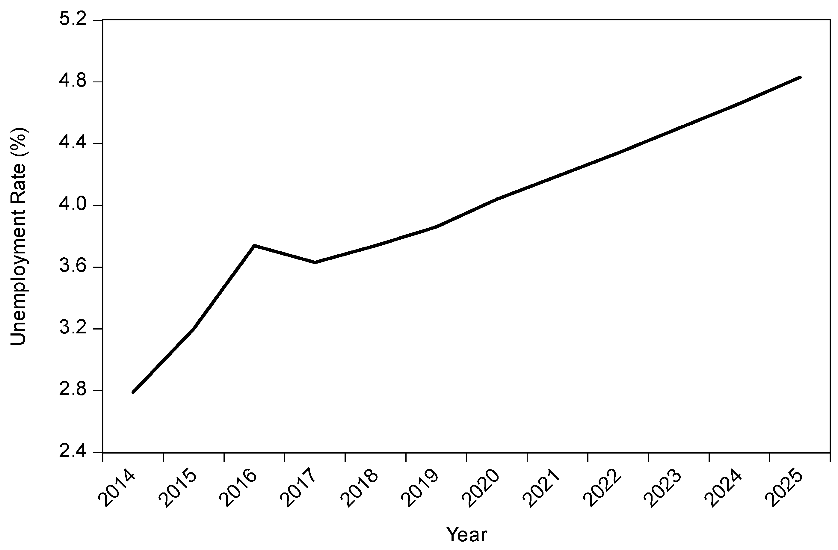
In Figure 12, The Mekong River Delta’s urban unemployment rate, which increased from 2.79% to 3.74% in the first three years, decreased slightly to 3.63% in 2017. However, it continued its upward trend to 3.86% in 2019 and is expected to rise to 4.83% in 2025.
In the Mekong River Delta’s rural area, the unemployment rate was estimated at 1.83% in 2014. The unemployment rate maintained at around 2.6% during three years from 2015 to 2018, and then experienced a decline to 2.37% in 2018. Last but not least, the unemployment rate increased to 2.6%. Nevertheless, estimations indicate that the unemployment rate in the Mekong River’s rural area would continue to decrease until 2025, and by 2025 the rate could be around 2.31% in Figure 13.

4.3. Comparative Analysis Results of the Proposed Models

The three models’ accuracies were tested through the MAPE. The performance of the proposed methods was investigated by comparing the initial values with x ^ ( 0 ) ( k ) and y ^ ( λ ) t . Details about the calculations of x ^ ( 0 ) ,   ε ( k ) ,   Δ ( k ) ,   Δ t can be explored in Equations (8), (17), and (21) for the GM (1,1), GVM, and ARIMA models, respectively.
According to Table 4 for estimated data, it is clarified that the errors of GM (1,1) are more accurate in comparison to that of GVM and ARIMA models. The average MAPE values of 5.88% for urban areas and 5.16% for rural areas in Table 4 are well fitted to the first level of the grade reference of the Grey prediction model, which is considered a highly accurate prediction. On the contrary, the MAPE values from the GVM and ARIMA models indicated significant errors (except HLR at the urban area in the ARIMA model) in the predictions for the future unemployment rate.
From Table 4, it is apparent that the predicted values have the lowest mean percentage errors. For the North Central region, the lowest mean percentage error is roughly 1.76%, which means the forecast was completely accurate with an accuracy of 98.24%. Meanwhile, the Highlands region results had a mean percentage error of 14.73% from the ARIMA (1,0,1) model, indicating forecasted reliability of 85.27%. The remaining reliability test results for other regions revolve around 2.25% to nearly 9%, considered highly accurate forecasting for GM (1,1) model.
It is shown in Table 4 that the mean percentage errors of the expected rural unemployment rate with GM (1,1) model in the North Central, Highlands, and Southeast Regions are relatively similar at 5.74%, 5.94%, and 5.57%, respectively. The Red River Delta’s figure is 4.53%, nearly twofold the number for the Mekong River Delta at 2.21%. However, the reliability test results of the estimated unemployment rates in the six regions are well fitted in the range of 1% to 10%.
Likewise, the MAPE results from the other administrative regions showed little-to-no errors in the GM (1,1) technique. This could be explained as, generally, the Traditional Grey Verhulst model could reflect the future unemployment rate; some defects in the model caused low predictions. This model indicated significant errors in the predictions for the future unemployment rate. However, the ARIMA model gave more successful forecastings than the Traditional Grey Verhulst model, except for RRD at the urban area and SER at the rural area.
As can be seen from the Appendices, the performance of the proposed methods was tested by comparing the initial values with g ^ ( 0 ) ( k ) and y ^ ( λ ) t . Details about the calculations of g ^ ( 0 ) ,   ε ( k ) ,   Δ ( k ) ,   Δ t can be explored in Equations (8), (9), (16) and (17) for the GM and GVM models and in Equations (20) and (21) for the ARIMA model (Appendix A, Appendix B, Appendix C, Appendix D and Appendix E).
Table 5 shows the unemployment rates for all regions’ urban and rural areas by using the GVM and ARIMA models. It is quite apparent that the unemployment rates for urban and rural areas would follow a downward trend until 2025 with the GVM model. On the contrary, the unemployment rates might steadily continue until 2025 with the ARIMA model.
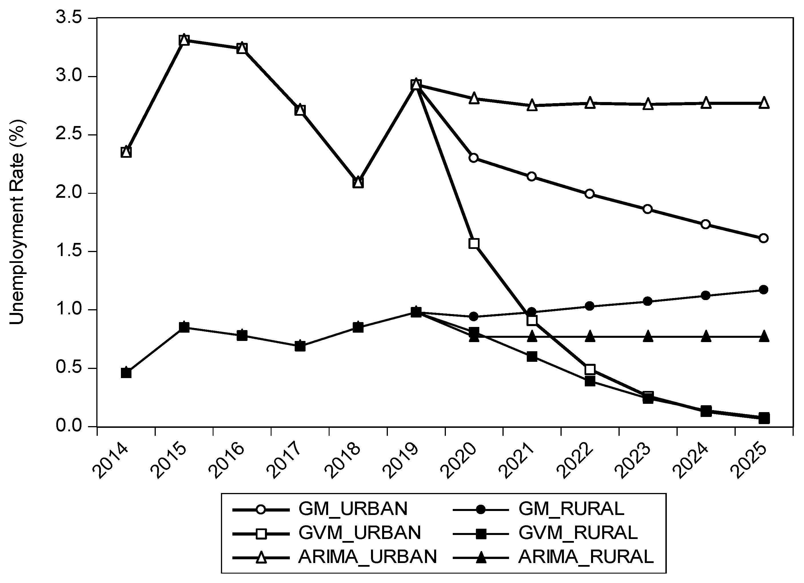
Figure 14 shows the comparisons of the average forecasted unemployment rates in the urban and rural areas for the GM, GVM, and ARIMA models. According to the GVM model’s forecasting between 2020 and 2025, the average forecasted unemployment rates in the urban and rural regions will reach 0.79 and 0.42, respectively. However, the average forecasted unemployment rates with the ARIMA model in urban regions range from approximately 3.1%, whereas the figures for the rural areas are 1.62%. The diagrams between Table A7 and Table A12 show the unemployment rates in whole regions for six years from 2020 to 2025 using three forecasting methods, separately.
5. Conclusions and Recommendations

5.1. Conclusions

Unemployment continues to be a significant source of economic decline in both developed and emerging countries, resulting in losing their aggregate financial and economic influence. Predicting unemployment rates attracted researchers’ interest within a short period. This study employed the GM (1,1), GVM, and ARIMA forecasting models to find the optimal technique for estimating the unemployment rate in Vietnam.
Forecast results indicated that the GM (1,1) is the optimal model for predicting Vietnam’s unemployment rate. The reason for choosing the GM (1,1) model is supported by an average MAPE of 5.88% for the forecast of the urban unemployment rate in Vietnam. The MAPE was calculated by comparing the forecast values with the initial values. Then, an error grade reference table was applied to assess the forecast model’s accuracy in the following step. It was clarified in the table that MAPE values ranging from below 10% to 10% could be perceived as highly accurate forecasting, except for the Highlands area. For this area, MAPE was found to be 14.94% with the GM (1,1) model, while the lowest value was seen at 14.73% from the ARIMA (1,0,1) model. On the opposite side, the MAPE of the urban unemployment rate using the GVM model was 17.17%, which was nearly three times that of the GM (1,1) model. However, the ARIMA model showed better performance than the GVM model with 10.41% as an average MAPE of the urban unemployment rate. According to the average MAPE of the rural unemployment rate results, the lowest value was found to be 5.16% in the GM (1,1) model. The GM (1,1) model was followed by the ARIMA model with 11.56% and the GVM model with 14.50%. In addition to the average results in rural areas, the GM (1,1) model was prominent enough that MAPE values ranging from below 7% could be perceived as highly accurate forecasting for all regions in rural.
According to the GM (1,1) model results, the unemployment rate for urban areas will follow a downward trend until 2025 except for MRD. The average unemployment rate of this area descends from more than 3% to 2.5% While the worst rate for MRD is 4.83% in 2025, in the same year, the rates of the rest of the regions from the highest to the lowest are NCR, SER, NMM, HLR, and RRD, respectively.
However, the mean unemployment rates of rural areas might continue to be relatively more stable than urban areas at approximately 1.5% levels. Our expectations show that the lowest unemployment rate will be seen in RRD or HLR between 2020 and 2025. NCR and MRD will exceed the mean of rural areas for the same sequence regularly.
The GM (1,1) model is evaluated in this study as the most successful strategy with a MAPE of around 5% (good forecasting results). As demonstrated by numerous previous studies, the GM (1,1) model has the following advantages: first, it is easy to calculate and requires less computing time; second, it requires a small number of data samples to generate reliable forecasts (generally, only four or more samples are required); and third, no prior series distribution is assumed.
However, the following are some disadvantages of the proposed approach. To begin, the GM (1,1) model uses the least-squares approach, resulting in skewed forecast results when the system has a high level of noise. Second, this approach is unsuitable for long-term forecasting.

5.2. Recommendations

Forecasting unemployment accurately is an essential challenge for policymakers since it is vital to a country’s financial and economic growth strategies. From the managerial perspective, the proposed forecasting model may be beneficial for financial institutions and policymakers to develop preference and strategy formulations. Results from the Grey Forecasting model identified an upward trend for the unemployment rate in most administrative regions. As shown in the illustrations for the Red River Delta, North Central, and Southeast regions, the unemployment rates for urban and rural areas in these three regions would continue to decrease as time goes on, maintaining at around between under 2% to above 3%. Supporting the trend is an influx way of Foreign Direct Investment (FDI). The number of newly registered investment projects was recorded at 606, amounting to USD 2,6 billion. In addition to that, capital-increasing projects accounted for about 62.5% of the region’s total FDI.
Moreover, accumulated calculations specified the number of 5800 registered projects since the ‘doi moi’ policy. In the Red River Delta, foreign investment projects made up 30% of total projects in Vietnam, accounting for approximately 26% of the total amount FDI in the country. The FDI data from a report in 2017 by the Foreign Direct Investment Department showed a significant increase in the number of new projects. It was estimated that in 2017, the Red River Delta had attracted nearly 7202 projects, which were worth USD 81,76 billion. Similarly, in recent years, the North Central region has attracted 402 projects with a total value of USD 32 billion, making up nearly 10% of the total FDI in Vietnam. This figure is relatively high as opposed to that of provinces in the South Central region.
Regarding the reasons for the region’s breakthrough, in addition to switching focus on developing synchronous infrastructure and proactively promoting investment opportunities, authorities in the North Central region also offer investment incentive policies towards administrative reform for foreign investors. Additionally, the GRDP in the agriculture, forestry, and fishery sector is less affected by the pandemic, experiencing an increase of 2.5% over the same period in 2019, higher than the whole country’s average of 1.19%; the GRDP in the construction sector also rose by 3.79% over the same period in 2019. Thanh Hoa and Quang Tri are the provinces with the highest GRDP growth at 3.7% and 4.17%, respectively. Meanwhile, the Southeast region experienced a GRDP growth of 7.9% in the first six months of 2019, above the nation’s average. As of 2020, the Southeast region makes up 60% of total foreign investment projects and nearly 50% of the total FDI; the region’s export turnover accounts for 60% of the country’s total export turnover.
Apart from attractive investment destinations such as the Red River Delta, the North Central, Southeast, Highlands, Northern Midlands and Mountains regions, and the Mekong River Delta stand in stark contrast with foreign investors’ low investment expectations. According to research co-conducted by Foreign Investment Department and United Nations Industrial Development Organization, they found up to 32% of foreign investors opt for the opinion that a shortage of high-skilled, discipline laborers is the main reason they cannot use up the full capacity of the machinery. On the one hand, since the Highlands region and the Mekong River Delta rely too much on agricultural business and the low quality of human capital, inadequate socioeconomic infrastructure, and very few vocational training centers and universities, the predictions for the unemployment rate in these regions are pretty pessimistic.
In general, increases in FDI growth over the past few years have created more job opportunities for thousands of workers. However, the FDI’s central focus in the regions mentioned above is on the garments and textiles industry, electrical device assembling, and real estate development. Moreover, disadvantaged regions are still struggling with attracting FDI due to internal difficulties. Consequently, domestic enterprises find it difficult to engage effectively in the global value chain, leading to the coordination between domestic and foreign companies not meeting expectations. In comparison to medium and high-skilled employees, young and low-skilled laborers are more prone to unemployment. This is because young and low-skilled laborers face a skills deficit. Thus, to attract further FDI, boost GDP, and alleviate unemployment in the following years, the Vietnamese government must build new labor markets that can alleviate the youth’s fixation with unemployment. A good example is a nightlife economy operating under the government’s control; this way, enterprises having business relationships with countries in different time zones could work 24 h a day. Simultaneously, Vietnamese authorities should also allocate finances to develop the logistics, ports, aviation, banking, and tourism industries. Specifically, the barriers in communicating in foreign languages and applying advanced technologies must be eliminated.

Author Contributions

Conceptualization, P.-H.N.; methodology, P.-H.N. and I.E.K.; software, P.-H.N. and I.E.K.; validation, J.-F.T.; formal analysis, J.-F.T.; investigation, P.-H.N.; resources, P.-H.N.; data curation, J.-F.T. and M.-H.L.; writing—original draft preparation, P.-H.N.; writing—review and editing, J.-F.T.; visualization, P.-H.N.; supervision, J.-F.T. and M.-H.L.; project administration, J.-F.T.; funding acquisition, J.-F.T. All authors have read and agreed to the published version of the manuscript.

Funding

This research was supported in part by the Ministry of Science and Technology in Taiwan under Grant MOST 109-2410-H-027-012-MY2.

Institutional Review Board Statement

The study was conducted according to the guidelines of the Declaration of Helsinki, and approved by the Institutional Review Board.

Informed Consent Statement

Informed consent was obtained from all subjects involved in the study.

Data Availability Statement

Not applicable.

Conflicts of Interest

Declare no conflict of interest.

Appendix A. Comparisons of the Proposed Methods for the Red River Delta Region

Table A1. Red River Delta—Urban area.
The Results of the Three Proposed Models (%)
Year g ( 0 ) ( k ) GM(1,1)GVMARIMA
g ^ ( 0 ) ( k ) ε(k)Δ(k) g ^ ( 1 ) ( k ) ε ( 1 ) ( k ) Δ(k) y ^ ( λ ) t Δ t p
20144.864.860.00000.0004.860.00000.0003.52cons.
20154.324.07−0.00230.0542.94−0.01360.3194.620.0070.000
20163.243.610.00370.1153.650.00410.1284.14AR (1)
20173.213.21−0.00000.0013.750.00540.1693.270.7950.003
20183.002.85−0.00160.0523.170.00170.0583.27
20192.532.53−0.00010.0022.27−0.00260.1023.11
Table A2. Red River Delta—Rural area.
The Results of the Three Proposed Models (%)
Year g ( 0 ) ( k ) GM(1,1)GVMARIMA
g ^ ( 0 ) ( k ) ε(k)Δ(k) g ^ ( 1 ) ( k ) ε ( 1 ) ( k ) g ^ ( 0 ) ( k ) y ^ ( λ ) t Δ t p
20141.841.840.00000.0001.840.00000.0001.70cons.
20152.202.08−0.00120.0541.31−0.00890.4031.730.0110.000
20161.731.870.00140.0781.780.00050.0291.87AR (1)
20171.641.670.00030.0191.970.00330.1991.700.3370.083
20181.441.500.00060.0401.740.00300.2081.67
20191.461.34−0.00120.0811.26−0.00200.1361.60

Appendix B. Comparisons of the Proposed Methods for the Northern Midlands and Mountains

Table A3. Northern Midlands and Mountains—Urban area.
The Results of the Three Proposed Models (%)
Year g ( 0 ) ( k ) GM(1,1)GVMARIMA
g ^ ( 0 ) ( k ) ε(k)Δ(k) g ^ ( 1 ) ( k ) ε ( 1 ) ( k ) g ^ ( 0 ) ( k ) y ^ ( λ ) t Δ t p
20142.352.350.00000.0002.350.00000.0002.77cons.
20153.313.27−0.00040.0121.83−0.01480.3192.730.0280.000
20163.243.05−0.00190.0592.68−0.00560.1282.84MA (1)
20172.712.840.00130.0483.230.00520.1692.78−1.0000.241
20182.092.650.00560.2663.110.01020.0582.76
20192.932.47−0.00470.1592.41−0.00520.1022.70
Table A4. Northern Midlands and Mountains—Rural area.
The Results of the Three Proposed Models (%)
Year g ( 0 ) ( k ) GM(1,1)GVMARIMA
g ^ ( 0 ) ( k ) ε(k)Δ(k) g ^ ( 1 ) ( k ) ε ( 1 ) ( k ) g ^ ( 0 ) ( k ) y ^ ( λ ) t Δ t p
20140.460.460.00000.0000.460.00000.0000.77cons.
20150.850.76−0.00090.1060.34−0.00510.6030.770.0080.000
20160.780.790.00010.0170.53−0.00250.3230.77MA (1)
20170.690.830.00140.2000.750.00060.0810.771.5460.000
20180.850.860.00010.0170.910.00060.0730.77
20190.980.90−0.00080.0790.94−0.00040.0420.77

Appendix C. Comparisons of the Proposed Methods for North Central

Table A5. North Central—Urban area.
The Results of the Three Proposed Models (%)
Year g ( 0 ) ( k ) GM(1,1)GVMARIMA
g ^ ( 0 ) ( k ) ε(k)Δ(k) g ^ ( 1 ) ( k ) ε ( 1 ) ( k ) g ^ ( 0 ) ( k ) y ^ ( λ ) t Δ t p
20143.713.710.00000.0003.710.00000.0004.03cons.
20154.144.190.00050.0114.10−0.00040.6034.190.0400.000
20164.284.14−0.00140.0334.280.00000.3234.09MA (1)
20174.034.100.00070.0174.030.00000.0813.89−1.3340.000
20183.954.060.00110.0273.950.00000.0733.96
20194.094.01−0.00080.0194.090.00000.0424.00
Table A6. North Central—Rural area.
The Results of the Three Proposed Models (%)
Year g ( 0 ) ( k ) GM(1,1)GVMARIMA
g ^ ( 0 ) ( k ) ε(k)Δ(k) g ^ ( 1 ) ( k ) ε ( 1 ) ( k ) g ^ ( 0 ) ( k ) y ^ ( λ ) t Δ t p
20141.701.700.00000.0001.700.00000.0001.98cons.
20151.902.030.00130.0661.28−0.00620.3292.040.0090.000
20162.172.02−0.00150.0681.86−0.00310.1412.05AR (1)
20171.952.020.00070.0362.290.00340.1761.980.5730.039
20182.222.02−0.00200.0912.290.00070.0331.98MA (1)
20191.862.010.00150.0831.860.00000.0011.91−1.0000.012

Appendix D. Comparisons of the Proposed Methods for the Highlands

Table A7. Highlands—Urban area.
The Results of the Three Proposed Models (%)
Year g ( 0 ) ( k ) GM(1,1)GVMARIMA
g ^ ( 0 ) ( k ) ε(k)Δ(k) g ^ ( 1 ) ( k ) ε ( 1 ) ( k ) g ^ ( 0 ) ( k ) y ^ ( λ ) t Δ t p
20141.941.940.00000.0001.940.00000.0002.15cons.
20152.842.51−0.00330.6911.34−0.01500.5302.240.0170.000
20162.182.350.00171.6971.91−0.00270.1251.91AR (1)
20171.982.190.00212.6912.340.00360.1821.930.2490.000
20181.512.050.00544.1342.390.00880.5842.06MA (1)
20192.521.91−0.00614.6422.03−0.00490.2952.46−1.0000.077
Table A8. Highlands—Rural area.
The Results of the Three Proposed Models (%)
Year g ( 0 ) ( k ) GM(1,1)GVMARIMA
g ^ ( 0 ) ( k ) ε(k)Δ(k) g ^ ( 1 ) ( k ) ε ( 1 ) ( k ) g ^ ( 0 ) ( k ) y ^ ( λ ) t Δ t p
20140.930.930.00000.0000.930.00000.00000.85cons.
20150.760.76−0.00000.0040.52−0.00240.31500.820.0060.000
20160.880.79−0.00090.1000.71−0.00170.19400.86AR (1)
20170.690.830.00140.2000.870.00180.25800.840.3280.000
20180.880.87−0.00010.0160.930.00050.06100.92MA (1)
20190.940.91−0.00030.0370.87−0.00070.07000.89−1.0000.077

Appendix E. Comparisons of the Proposed Methods for the Southeast Region

Table A9. Southeast Region—Urban area.
The Results of the Three Proposed Models (%)
Year g ( 0 ) ( k ) GM(1,1)GVMARIMA
g ^ ( 0 ) ( k ) ε(k)Δ(k) g ^ ( 1 ) ( k ) ε ( 1 ) ( k ) g ^ ( 0 ) ( k ) y ^ ( λ ) t Δ t p
20143.003.000.00000.0003.000.00000.0002.88cons.
20153.082.88−0.00200.0641.88−0.01200.3892.850.0180.000
20162.622.880.00260.0972.60−0.00020.0092.78AR (1)
20172.822.870.00050.0163.120.00300.1062.910.3920.000
20182.932.86−0.00070.0253.180.00250.0862.95MA (1)
20192.882.85−0.00030.0112.75−0.00130.0462.93−1.0000.062
Table A10. Southeast Region—Rural area.
The Results of the Three Proposed Models (%)
Year g ( 0 ) ( k ) GM(1,1)GVMARIMA
g ^ ( 0 ) ( k ) ε(k)Δ(k) g ^ ( 1 ) ( k ) ε ( 1 ) ( k ) g ^ ( 0 ) ( k ) y ^ ( λ ) t Δ t p
20141.601.600.00000.0001.600.00000.0002.06cons.
20152.262.370.00110.0481.40−0.00860.3832.080.0210.000
20162.202.260.00060.0262.11−0.00090.0392.06AR (1)
20172.452.15−0.00300.1222.570.00120.0502.06−0.0260.000
20182.112.05−0.00060.0282.410.00300.1422.05
20191.761.960.00190.11071.760.00000.0022.06

Appendix F. Comparisons of the Proposed Methods for the Mekong River Delta Region

Table A11. Mekong River Delta Region—Urban area.
The Results of the Three Proposed Models (%)
Year g ( 0 ) ( k ) GM(1,1)GVMARIMA
g ^ ( 0 ) ( k ) ε(k)Δ(k) g ^ ( 1 ) ( k ) ε ( 1 ) ( k ) g ^ ( 0 ) ( k ) y ^ ( λ ) t Δ t p
20142.792.7900.00000.0002.7900.00000.0003.49cons.
20153.206.169−2.96900.9282.0461.15400.3613.000.0100.000
20163.749.671−5.93101.5863.0490.69060.1853.29AR (1)
20173.6313.300−9.67002.6643.928−0.29830.0823.670.7080.000
20183.7417.061−13.32103.5624.209−0.46940.1263.59
20193.8620.959−17.09904.4303.7070.15270.0403.67
Table A12. Mekong River Delta Region—Rural area.
The Results of the Three Proposed Models (%)
Year g ( 0 ) ( k ) GM(1,1)GVMARIMA
g ^ ( 0 ) ( k ) ε(k)Δ(k) g ^ ( 1 ) ( k ) ε ( 1 ) ( k ) g ^ ( 0 ) ( k ) y ^ ( λ ) t Δ t p
20141.831.830.00000.0001.830.00000.0002.45cons.
20152.644.47−0.01830.6911.441.19550.4532.660.0170.000
20162.627.07−0.04451.6972.190.42920.1642.52AR (1)
20172.619.63−0.07022.6912.81−0.20250.0782.420.3180.000
20182.3712.17−0.09804.1342.93−0.55870.2362.34MA (1)
20192.6014.67−0.12074.6422.450.14550.0562.40−1.0000.041
Figure A1. Comparisons of forecasted unemployment rates in urban and rural areas of the Northern Midlands and Mountains for three models.
Sustainability 13 07879 g0a1
Figure A2. Comparisons of forecasted unemployment rates in urban and rural areas of the North Central region for three models.
Sustainability 13 07879 g0a2
Figure A3. Comparisons of forecasted unemployment rates in urban and rural areas of the Highlands for three models.
Sustainability 13 07879 g0a3
Figure A4. Comparisons of forecasted unemployment rates in urban and rural areas of the South East Region for three models.
Sustainability 13 07879 g0a4
Figure A5. Comparisons of forecasted unemployment rates in urban and rural areas of the Mekong River Delta Region for three models.
Sustainability 13 07879 g0a5

References

  1. Couch, K.A.; Fairlie, R.W.; Xu, H. Early evidence of the impacts of COVID-19 on minority unemployment. J. Public Econ. 2020, 192, 104287. [Google Scholar] [CrossRef]
  2. Christiano, L.; Trabandt, M.; Walentin, K. Involuntary Unemployment and the Business Cycle. Rev. Econ. Dyn. 2010, 39, 26–54. [Google Scholar] [CrossRef]
  3. Stauder, J. Unemployment, unemployment duration, and health: Selection or causation? Eur. J. Health Econ. 2018, 20, 59–73. [Google Scholar] [CrossRef]
  4. Nguyen, P.-H.; Tsai, J.-F.; Nguyen, H.-P.; Nguyen, V.-T.; Dao, T.-K. Assessing the Unemployment Problem Using a Grey MCDM Model under COVID-19 Impacts: A Case Analysis from Vietnam. J. Asian Financ. Econ. Bus. 2020, 7, 53–62. [Google Scholar] [CrossRef]
  5. Giang, N.T. Long-run Relationship of Economic Growth with Consumption, Unemployment Rates and Saving Rates in Developing Countries: A Case Study of Vietnam. J. Bus. Manag. Sci. 2020, 8, 61–66. [Google Scholar]
  6. Petrosky-Nadeau, N.; Zhang, L. Unemployment Crises. J. Monet. Econ. 2013, 117, 335–353. [Google Scholar] [CrossRef]
  7. Ahn, H.J.; Hamilton, J.D. Heterogeneity and Unemployment Dynamics. J. Bus. Econ. Stat. 2016, 38, 554–569. [Google Scholar] [CrossRef] [Green Version]
  8. Carrère, C.; Fugazza, M.; Olarreaga, M.; Robert-Nicoud, F. Comparative advantage and equilibrium unemployment. Eur. Econ. Rev. 2020, 127, 103496. [Google Scholar] [CrossRef]
  9. Blustein, D.L.; Duffy, R.; Ferreira, J.; Cohen-Scali, V.; Cinamon, R.G.; Allan, B.A. Unemployment in the time of COVID-19: A research agenda. J. Vocat. Behav. 2020, 119, 103436. [Google Scholar] [CrossRef]
  10. Cazzola, A.; Pasquini, L.; Angeli, A. The relationship between unemployment and fertility in Italy: A time-series analysis. Demogr. Res. 2016, 34, 1–38. [Google Scholar] [CrossRef] [Green Version]
  11. Ullah, M.N.; Su, K.K.; Jan, B. Forecasting, Cointegration and Causality Analysis of Unemployment Using Time Series Models. SSRN Electron. J. 2017. [Google Scholar] [CrossRef]
  12. Chang, S.-S.; Sterne, J.; Huang, W.-C.; Chuang, H.-L.; Gunnell, D. Association of secular trends in unemployment with suicide in Taiwan, 1959–2007: A time-series analysis. Public Health 2010, 124, 49–54. [Google Scholar] [CrossRef] [PubMed]
  13. Chakraborty, T.; Chakraborty, A.K.; Biswas, M.; Banerjee, S.; Bhattacharya, S. Unemployment Rate Forecasting: A Hybrid Approach. Comput. Econ. 2021, 57, 183–201. [Google Scholar] [CrossRef]
  14. Green, A.E.; Owen, D.W.; Winnett, C.M. The Changing Geography of Recession: Analyses of Local Unemployment Time Series. Trans. Inst. Br. Geogr. 1994, 19, 142. [Google Scholar] [CrossRef]
  15. Ayinde, O.E. Empirical Analysis of Agricultural Growth and Unemployment in Nigeria. Afr. J. Agric. Res. 2008, 3, 465–468. [Google Scholar]
  16. Schaal, E. Uncertainty and Unemployment. Econometrica 2017, 85, 1675–1721. [Google Scholar] [CrossRef]
  17. Katris, C. Prediction of Unemployment Rates with Time Series and Machine Learning Techniques. Comput. Econ. 2019, 55, 673–706. [Google Scholar] [CrossRef]
  18. JLuna-Romera, M.; Núñez-Hernández, F.; Martínez-Ballesteros, M.; Riquelme, J.C.; Ibáñez, C.U. Analysis of the evolution of the Spanish labour market through unsupervised learning. IEEE Access 2019, 7, 121695–121708. [Google Scholar] [CrossRef]
  19. Cockx, B.; Lechner, M.; Bollens, J. Priority to Unemployed Immigrants? A Causal Machine Learning Evaluation of Training in Belgium (2020). CESifo Working Paper No. 8297. Available online: https://ssrn.com/abstract=3603832 (accessed on 20 May 2020).
  20. Hall, A.S. Machine Learning Approaches to Macroeconomic Forecasting. Fed. Reserv. Bank Kans. City Econ. Rev. 2018, 103, 2. [Google Scholar] [CrossRef]
  21. Kreiner, A.; Duca, J.V. Can machine learning on economic data better forecast the unemployment rate? Appl. Econ. Lett. 2020, 27, 1434–1437. [Google Scholar] [CrossRef] [Green Version]
  22. Adam, A.M.A.M.T.; Abd Allah, B. Estimating the Determinants of Unemployment in Sudan by Applying the Philips Curve Using the E GARCH Model during the Period 1990–2018. Int. J. Innov. Sci. Res. Technol. 2020, 5, 172–178. [Google Scholar]
  23. Abouelfarag, H.A.; Qutb, R. Does government expenditure reduce unemployment in Egypt? J. Econ. Adm. Sci. 2020. [Google Scholar] [CrossRef]
  24. Misra, A.; Singh, A.K. A mathematical model for unemployment. Nonlinear Anal. Real World Appl. 2011, 12, 128–136. [Google Scholar] [CrossRef]
  25. Al-Maalwi, R.; Al-Sheikh, S.; Ashi, H.; Asiri, S. Mathematical modeling and parameter estimation of unemployment with the impact of training programs. Math. Comput. Simul. 2021, 182, 705–720. [Google Scholar] [CrossRef]
  26. Shimer, R. Reassessing the Ins and Outs of Unemployment. Rev. Econ. Dyn. 2007, 15, 127–148. [Google Scholar] [CrossRef] [Green Version]
  27. Dritsakis, N.; Klazoglou, P. Forecasting Unemployment Rates in USA Using Box-Jenkins Methodology. Int. J. Econ. Financ. Issues 2018, 8, 9–20. [Google Scholar]
  28. Victor, V.; Karakunnel, J.; Loganathan, S.; Meyer, D. From a Recession to the COVID-19 Pandemic: Inflation–Unemployment Comparison between the UK and India. Economies 2021, 9, 73. [Google Scholar] [CrossRef]
  29. Bedowska-Sojka, B. Unemployment Rate Forecasts: Evidence from the Baltic States. East. Eur. Econ. 2015, 53, 57–67. [Google Scholar] [CrossRef]
  30. Claveria, O. Forecasting the unemployment rate using the degree of agreement in consumer unemployment expectations. J. Labour Mark. Res. 2019, 53, 3. [Google Scholar] [CrossRef] [Green Version]
  31. Ahmad, M.; Khan, Y.A.; Jiang, C.; Kazmi, S.J.H.; Abbas, S.Z. The impact of COVID-19 on unemployment rate: An intelligent based unemployment rate prediction in selected countries of Europe. Int. J. Finance Econ. 2021, 1–16. [Google Scholar] [CrossRef]
  32. Davidescu, A.; Apostu, S.-A.; Paul, A. Comparative Analysis of Different Univariate Forecasting Methods in Modelling and Predicting the Romanian Unemployment Rate for the Period 2021–2022. Entropy 2021, 23, 325. [Google Scholar] [CrossRef]
  33. Gil-Alana, L. A fractionally integrated exponential model for UK unemployment. J. Forecast. 2001, 20, 329–340. [Google Scholar] [CrossRef] [Green Version]
  34. Wong, J.M.W.; Chan, A.P.C.; Chiang, Y.H. Time series forecasts of the construction labour market in Hong Kong: The Box-Jenkins approach. Constr. Manag. Econ. 2005, 23, 979–991. [Google Scholar] [CrossRef]
  35. Naccarato, A.; Falorsi, S.; Loriga, S.; Pierini, A. Combining official and Google Trends data to forecast the Italian youth unemployment rate. Technol. Forecast. Soc. Chang. 2018, 130, 114–122. [Google Scholar] [CrossRef]
  36. Liu, S.; Heinzel, S.; Haucke, M.; Heinz, A. Increased Psychological Distress, Loneliness, and Unemployment in the Spread of COVID-19 over 6 Months in Germany. Medicina 2021, 57, 53. [Google Scholar] [CrossRef]
  37. Khemka, G.; Roberts, S.; Higgins, T. The Impact of Changes to the Unemployment Rate on Australian Disability Income Insurance Claim Incidence. Risks 2017, 5, 17. [Google Scholar] [CrossRef] [Green Version]
  38. Simionescu, M.; Streimikiene, D.; Strielkowski, W. What Does Google Trends Tell Us about the Impact of Brexit on the Unemployment Rate in the UK? Sustainability 2020, 12, 1011. [Google Scholar] [CrossRef] [Green Version]
  39. Hu, Y.-C.; Jiang, P.; Chiu, Y.-J.; Tsai, J.-F. A Novel Grey Prediction Model Combining Markov Chain with Functional-Link Net and Its Application to Foreign Tourist Forecasting. Information 2017, 8, 126. [Google Scholar] [CrossRef] [Green Version]
  40. Julong, D. Introduction to grey system. J. Grey Syst. 1989, 1, 1–24. [Google Scholar]
  41. Liu, S.; Lin, Y. Introduction to Grey Systems Theory. Underst. Complex Syst. 2010, 68, 1–18. [Google Scholar] [CrossRef]
  42. Liu, S.; Yang, Y.; Forrest, J. Series of GM Models. In Grey Data Analysis: Methods, Models and Applications; Springer: Singapore, 2017; pp. 141–181. [Google Scholar]
  43. Submitted, T. A Grey Verhulst Model for Forecasting Construction Costs; ProQuest LLC: Ann Arbor, MI, USA, 2020. [Google Scholar]
  44. Zhou, W.; Pei, L. The grey generalized Verhulst model and its application for forecasting Chinese pig price index. Soft Comput. 2020, 24, 4977–4990. [Google Scholar] [CrossRef]
  45. Nguyen, N.-T.; Tran, T.-T. Optimizing mathematical parameters of Grey system theory: An empirical forecasting case of Vietnamese tourism. Neural Comput. Appl. 2017, 31, 1075–1089. [Google Scholar] [CrossRef]
  46. Zeng, B.; Tong, M.; Ma, X. A new-structure grey Verhulst model: Development and performance comparison. Appl. Math. Model. 2020, 81, 522–537. [Google Scholar] [CrossRef]
  47. Tang, L.; Lu, Y. Study of the grey Verhulst model based on the weighted least square method. Phys. A Stat. Mech. Its Appl. 2020, 545, 123615. [Google Scholar] [CrossRef]
  48. Karaaslan, A.; Özden, K. Özgür Housing Demand in Turkey: Application of Grey Forecasting Model. Mediterr. J. Soc. Sci. 2016, 7, 52–62. [Google Scholar] [CrossRef] [Green Version]
  49. Box, G.E.P.; Jenkins, G.M. Control; Halden-Day: San Francisco, CA, USA, 1970. [Google Scholar]
Figure 1. Comparison of the average forecasted unemployment rates in urban and rural areas with GM (1,1).
Sustainability 13 07879 g001
Figure 2. Predicted unemployment rate for the urban area of the Red River Delta with GM (1,1) for the period from 2020 to 2025.
Sustainability 13 07879 g002
Figure 3. Predicted unemployment rate for the rural area of the Red River Delta with GM (1,1) for the period from 2020 to 2025.
Sustainability 13 07879 g003
Figure 4. Predicted unemployment rate for the urban area of the Northern Midlands and Mountains with GM (1,1) for the period from 2020 to 2025.
Sustainability 13 07879 g004
Figure 5. Predicted unemployment rate for the rural area of the Northern Midlands and Mountains with GM (1,1) for the period from 2020 to 2025.
Sustainability 13 07879 g005
Figure 6. Predicted unemployment rate for the urban area of the North Central Region with GM (1,1) for the period from 2020 to 2025.
Sustainability 13 07879 g006
Figure 7. Predicted unemployment rate for the rural area of the North Central Region with GM (1,1) for the period from 2020 to 2025.
Sustainability 13 07879 g007
Figure 8. Predicted unemployment rate for the urban area of the Highlands Region with GM (1,1) for the period from 2020 to 2025.
Sustainability 13 07879 g008
Figure 9. Predicted unemployment rate for the rural area of the Highlands Region with GM (1,1) for the period from 2020 to 2025.
Sustainability 13 07879 g009
Figure 10. Predicted unemployment rate for the urban area of the Southeast Region with GM (1,1) for the period from 2020 to 2025.
Sustainability 13 07879 g010
Figure 11. Predicted unemployment rate for the rural area of the Southeast Region with GM (1,1) for the period from 2020 to 2025.
Sustainability 13 07879 g011
Figure 12. Predicted unemployment rate for the urban area of the Mekong River Delta with GM (1,1) model for the period from 2020 to 2025.
Sustainability 13 07879 g012
Figure 13. Predicted unemployment rate for the rural area of the Mekong River Delta with GM (1,1) model for the period from 2020 to 2025.
Sustainability 13 07879 g013
Figure 14. Comparisons of average forecasted unemployment rates in urban and rural areas for three models.
Sustainability 13 07879 g014
Table 1. MAPE value efficiencies in forecasting results.
MAPE (%)Forecast Results
<10Highly accurate results
10–20Good results
20–50Reasonable results
>50Weak and inaccurate results
Table 2. Actual and forecasted unemployment rate using GM (1,1) in Urban Areas (%).
NoRegionsUnemployment Rate—Urban Areas (%)
Years201420152016201720182019202020212022202320242025
1RRDActual4.864.323.243.213.002.53
Forecasted4.864.073.613.212.852.532.241.991.771.571.391.23
2NMMActual2.353.313.242.712.092.93
Forecasted2.353.273.052.842.652.472.302.141.991.861.731.61
3NCRActual3.714.144.284.033.954.09
Forecasted3.714.194.144.104.064.013.973.933.893.853.813.77
4HLRActual1.942.842.181.981.512.52
Forecasted1.942.512.352.192.051.911.791.671.561.461.361.27
5SERActual3.003.082.622.822.932.88
Forecasted3.002.882.882.872.862.852.842.832.822.812.802.79
6MRDActual2.793.203.743.633.743.86
Forecasted2.794.044.194.344.504.664.044.194.344.504.664.83
Average Forecast3.113.493.373.263.173.072.862.792.732.672.622.58
Table 3. Actual and forecasted unemployment rate using GM (1,1) in Rural Areas (%).
NoRegionsUnemployment Rate—Rural Areas (%)
Years201420152016201720182019202020212022202320242025
1RRDActual1.842.201.731.641.441.46
Forecasted1.842.081.871.671.501.341.201.080.970.870.780.70
2NMMActual0.460.850.780.690.850.98
Forecasted0.460.760.790.830.860.900.940.981.031.071.121.17
3NCRActual1.701.902.171.952.221.86
Forecasted1.702.032.022.022.022.012.012.012.012.002.002.00
4HLRActual0.930.760.880.690.880.94
Forecasted0.930.760.790.830.870.910.950.991.041.081.131.18
5SERActual1.602.262.202.452.111.76
Forecasted1.602.372.262.152.051.961.861.781.691.611.541.47
6MRDActual1.832.642.622.612.372.60
Forecasted1.832.472.442.412.382.342.472.442.412.382.342.31
Average Forecast1.391.751.701.651.611.581.571.551.531.501.491.47
Table 4. Comparisons of MAPE of the proposed methods (%).
UrbanGM (1,1)GVMARIMAARIMA MAPE
RRD3.72 *13.00(1,0,0)16.67
NMM9.06 *25.00(0,0,1)14.12
NCR1.76 *14.00(0,0,1)3.74
HLR14.9427.00(1,0,1)14.73 *
SER3.56 *11.00(1,0,1)4.25
MRD2.25 *13.00(1,0,0)8.96
Average5.8817.17 10.41
RuralGM (1,1)GVMARIMAARIMA MAPE
RRD4.53 *16.00(1,0,0)11.42
NMM6.99 *19.00(0,0,1)20.12
NCR5.74 *11.00(1,0,1)7.06
HLR5.94 *15.00(1,0,1)8.44
SER5.57 *10.00(1,0,0)13.23
MRD2.21 *16.00(1,0,1)9.10
Average5.1614.50 11.56
* most accurate model.
Table 5. Forecasted unemployment rate using the GVM and ARIMA models for the urban and rural areas (%).
NoRegionsUnemployment Rate (%)
GVMARIMA
Areas202020212022202320242025202020212022202320242025
1RRDUrban1.440.840.470.260.140.072.712.873.013.113.193.26
Rural0.790.450.240.130.060.031.631.681.691.701.701.70
2NMMUrban1.570.910.490.260.130.072.812.752.772.762.772.77
Rural0.810.600.390.240.140.080.770.770.770.770.770.77
3NCRUrban2.691.690.980.550.300.163.964.034.034.034.034.03
Rural1.270.770.430.230.120.061.951.961.971.981.981.98
4HLRUrban1.470.940.560.320.170.102.202.162.152.152.152.15
Rural0.720.530.360.230.140.090.840.840.850.850.850.85
5SERUrban2.051.370.850.500.290.162.922.902.892.892.882.88
Rural1.070.580.290.140.070.032.072.062.062.062.062.06
6MRDUrban2.741.781.060.590.320.173.753.683.623.593.563.54
Rural1.711.040.590.310.160.082.322.402.432.442.442.45
Publisher’s Note: MDPI stays neutral with regard to jurisdictional claims in published maps and institutional affiliations.