The Impact of Indoor Living Wall System on Air Quality: A Comparative Monitoring Test in Building Corridors

Abstract

Living wall systems have been widely recognized as one of the promising approaches for building applications due to their aesthetic value and ecological benefits. Compared with outdoor living wall systems, indoor living wall systems (ILWS) play a more vital role in indoor air quality. The aim of this study is to investigate the effects of ILWS on indoor air quality. In an office building, two parallel corridors were selected as comparative groups. A 10.6 m² ILWS was installed on the sidewall of the west corridor while the east corridor was empty. Some important parameters, including indoor air temperature, relative humidity, concentrations of carbon dioxide (CO₂), and particulate matter (PM) were obtained based on the actual environment monitoring. According to the statistical analysis of the data, there were significant differences in the concentrations of CO₂ and PMs in the corridors with and without ILWS, which indicated that CO₂ and PM_2.5 removal rate ranged from 12% to 17% and 8% to 14%, respectively. The temperature difference is quite small (0.13 °C on average), while relative humidity slightly increased by 3.1–6.4% with the presence of the ILWS.

1. Introduction

Currently, city development trends in the vertical direction owing to the rapid increase in population, especially in developing countries [1,2]. The growth of density and reduction of green spaces has caused a series of urban environmental health problems including the heat island effect [3] and air particle pollution [4]. In recent years, the purification and thermal effects of green plants on the urban environment have received increasing attention in the academic community [5,6,7]. Their ecological effects have also been verified, such as pollution reduction [8,9], noise reduction [10,11,12], increase in biodiversity [13,14,15], and energy consumption reduction [16,17,18,19,20,21,22]. Relevant research studies are mostly focused on outdoor greening, such as three-dimensional greening in urban centers [23], greening of roofs [24], and building skins [25]. Hence, the vertical greenery system (VGS) becomes an ideal typology of greening in a crowded city, since it effectively uses the vertical space to accommodate the green plants. VGS can be categorized into green façade and the living wall system (LWS) based on structure configurations. A green façade refers to the climbing plants rooting at the ground level. The vegetation can either climb on the wall directly or indirectly with trellises. By contrast, an LWS refers to vegetation grown in felt or modular systems attached to the walls. The felt or modular system holds the substrate media which can be watered mechanically [26]. With a number of planting units, LWS can be flexibly pixilated with species of colorful plants to form a green pattern which could add aesthetic value to the built environment [27].

Generally, LWS can be divided into two categories including outdoor living wall system (OLWS) and indoor living wall system (ILWS) [26]. In recent years, OLWS has been widely investigated and conducted to verify the potential in terms of thermal enhancement and energy-saving. Results show that the OLWS can effectively improve thermal comfort and decrease energy demand in summer and act as extra insulation in winter [28,29,30,31].

Compared with OLWS, the studies on ILWS are quite limited. Previous papers of ILWS focus on thermal comfort and energy-saving aspects [32]. There is little attention given to ILWSs’ impact on the indoor physical environment, especially indoor air quality. López-Aparicio et al. [33] found that the deterioration of outdoor air quality could indirectly affect indoor air quality. The most prominent indoor air pollutants are carbon dioxide (CO₂), particulate matter (PM), and a range of volatile organic compounds (VOCs) [34]. An elevated level of CO₂ concentration has been associated with “sick building syndrome”. When CO₂ concentration rises from 389 ppm to 1160 ppm, sick building symptoms will increase significantly [35]. The CO₂ concentration also has an effect on workplace productivity. Research shows that when the indoor CO₂ concentration reduced from 1515 ppm to 735 ppm, the human reaction time was shortened by 5.4% [36]. Long-term exposure to high concentrations of PMs (higher than 50 μg/m³) could lead to the increasing of morbidity and mortality due to cardiovascular, respiratory, and venous thromboembolic diseases [37]. VOCs have also been associated with several health effects according to different main ingredients [34]. As a majority of citizens spend almost 90% of their time indoors every day [38], ensuring good indoor air quality becomes a prerequisite for people to maintain a healthy state of daily life. Although small in number, studies have been done to investigate the impact of green walls on indoor environmental quality, including CO₂ and PMs concentration, temperature, and humidity. Ghazalli et al. [39] studied the impact of IVGS installation in the north-south corridor on PMs, temperature, and humidity, and found that IVGS has no significant impact on temperature but can reduce particulate matter concentration and increase indoor humidity. Su and Lin [40] showed that a 5.72 m² ILWS could reduce the CO₂ concentration of a 38.88 m³ room from 2000 to 800 ppm within 4 h. Torpy et al. [41] showed that a 1 m² ILWS was capable of significant room CO₂ reductions, but only with considerable supplementary lighting (250 mmol/m²/s), whilst indoor light levels typically range between 5 and 12 mmol/m²/s. Tudiwer et al. [42] tested a 5.88 m² ILWS installed on the sidewall of a classroom (8.5m Length × 6.5 m Width × 3.7 m Height) and found that compared with non-green classrooms, the relative humidity of the green classroom increased by 34.21%, and the indoor CO₂ concentration decreased by 3.5%. The comfort level was increased by 20.6% (the local comfort zone: temperature 17 °C to 25.5 °C, relative humidity 18% to 87%).

At present, there are only a few academic research studies on the effect of ILWS on indoor air pollutant removal and thermal comfort enhancement. Research in its impact on different parameters, including the concentration of CO₂, the concentration of PMs, temperature, and humidity, at different climatic zones is needed. The purpose of this paper is to fill this knowledge gap by providing a ten-month monitoring test and statistical analysis within an office building at Cfa climatic zone (the subtropical climate and the precipitation more evenly distributed throughout the year) in Köppen climate classification. Two parallel corridors, with and without ILWS, were investigated to assess the effects of ILWS on indoor air pollutant reduction (CO₂ and PMs concentration) and thermal condition (temperature and relative humidity).

2. Methods

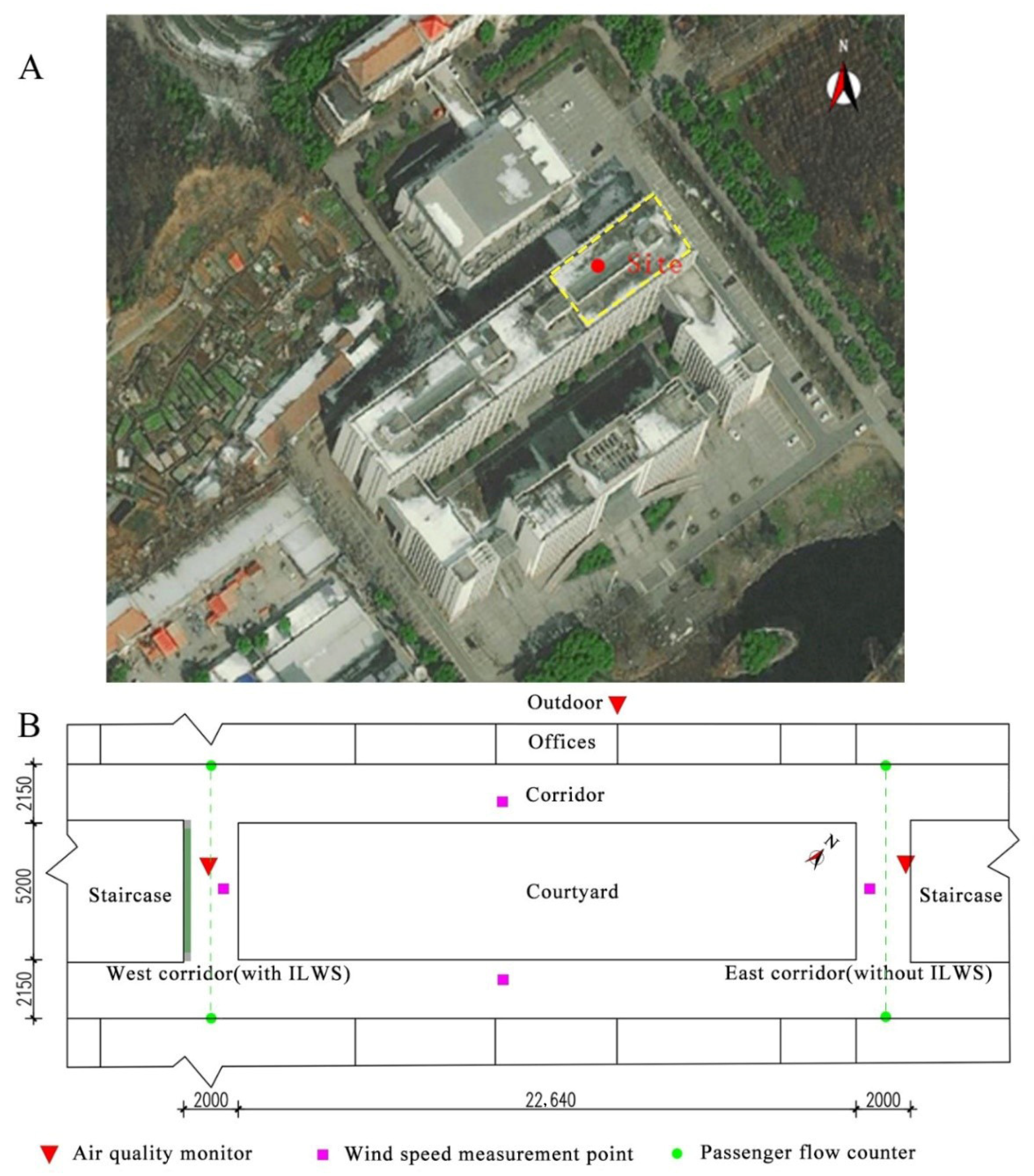
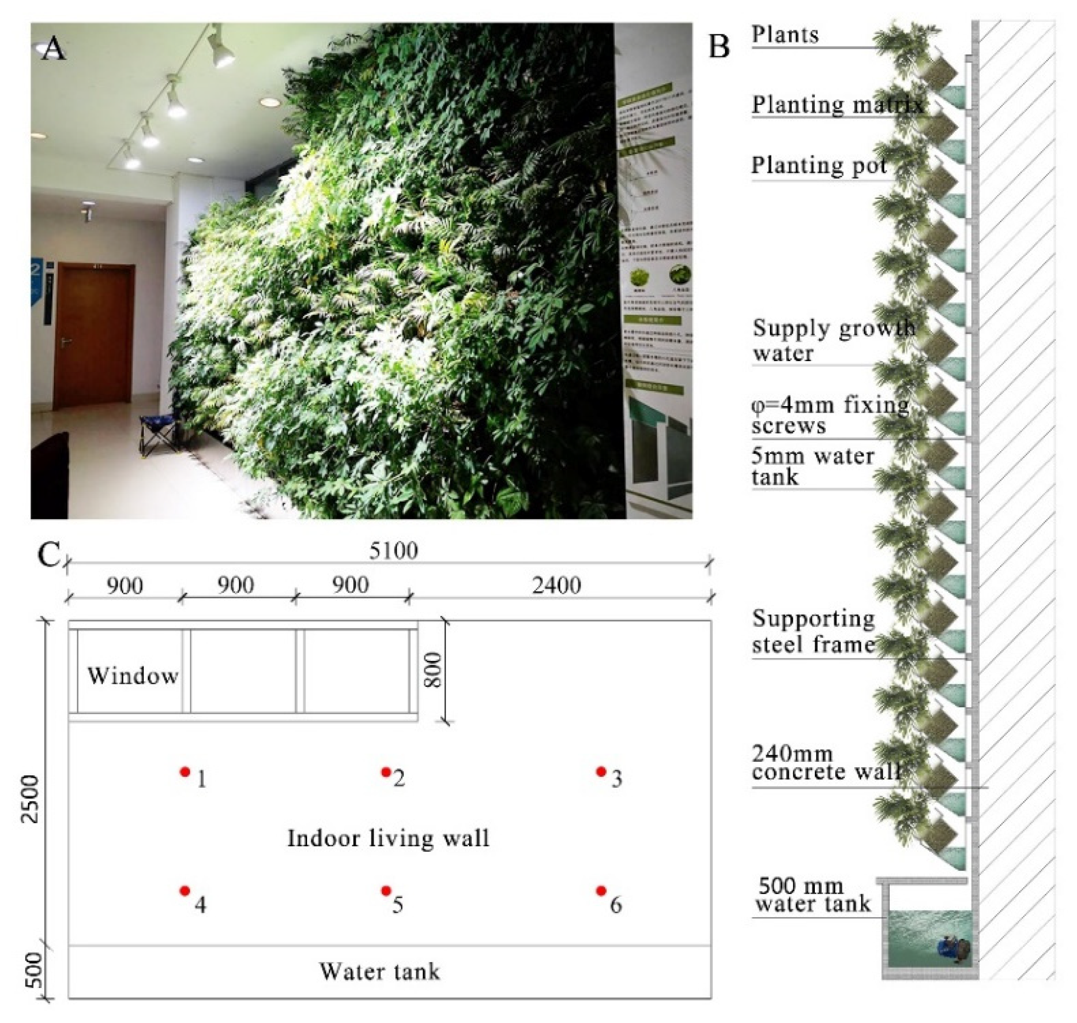
2.1. Location of the Study

The site is located in Nanjing city (118°38′24″ E, 32°04′48″ N), which is situated in the hot summer and cold winter climatic zone. Based on the China Meteorological Data Network [43], as shown in Figure 1, the maximum ambient air temperature is about 37.2 °C in July, while the minimum is −5.6 °C in January. In terms of relative humidity, despite the large fluctuations from 15% to 100%, most of the values are concentrated in the 60–90% range, with an average of over 70%.

2.2. Monitoring Conditions

The monitoring test was carried out on the first floor of a six-story office building (built in 2010) at the university park as shown in Figure 2. To be more specific, the ILWS is arranged on the wall of the stairwell at the western end of the corridor, which has an area of approximately 10.6 m² as shown in Figure 3. The ILWS has been constructed and run for more than 2 years. The ILWS consists of a modular planting pot array, a drip irrigation network, and a light-emitting diode (LED) lighting system. Specifically, the water at the bottom of the tank is pumped to each level of the planting pot array, which is then distributed by the drip irrigation to each pot and finally circulated back to the water tank by gravity. The vegetation of ILWS consists of three shade-requiring landscaping plants (

Table 1. Plants on the indoor living wall system.

Name of the Plant	Light Requirement	Growth Cycle Category	Applied Area (m2)/Proportion (%)
Schefflera octophylla (Lour.) Harms	shade-loving	Perennial	5.2/49.1%
Fatsia japonica (Thunb.) Decne. et Planch	shade-loving	Perennial	2.1/19.8%
Chamaedorea elegans Mart	shade-loving	Perennial	3.3/31.1%

). By contrast, the wall without ILWS is at the eastern end of the corridor. The corridors are enclosed by glazing that separates the indoor corridor space from the courtyard. The building information can be found in

Table 2. Building information.

Building Components	Specifications
Floor height	4 m, floor to floor height
Wall	240 mm hollow concrete small blocks wall with paint finish
Ceiling	light steel keel asbestos board suspended ceiling
Floor	120 mm cast-in-place concrete with floor tile finish
Glazing	6 mm single glazing
HVAC system	no HVAC system in corridors and other public spaces, single air-conditioner in separated offices

.

2.3. Monitored Parameters and Sensors

A series of parameters, including CO₂ and PMs concentration, temperature, and relative humidity, of the two corridors, were compared using recorded monitoring data. In doing this, several devices were adopted, including three air quality monitors, a photosynthetically active radiation (PAR) meter, two anemometers, and two pairs of passenger flow counters, as presented in Figure 4.

Table 3. Parameters measurement and methods.

Parameters	Devices	Type	Measurement Method	Accuracy
CO2 (ppm)	Air quality monitor (BohuBH-03)	SenseonAir S8 PMS7003 Senseon SHT20	7/24 h, automatic recording frequency is 1 time/min	±3%
PM0.3–1 (μg/m3)				±2%
PM1–2.5 (μg/m3)				±2%
PM2.5–10 (μg/m3)				±2%
Temperature (°C)				±0.2 °C
Relative humidity (%)				±2%
PPFD (μmol/s)	PAR meter	Apogee MQ-500	Manual measurement	±5%
Dimension (m)	Laser rangefinder	Bosch GLM30	Manual measurement	±1.0 mm
Wind speed (m/s)	Digital anemometer	PM6252B	7/24 h, automatic recording frequency is 1 time/15 min	±2%
Human traffic	Passenger flow counter	iDTK	7/24 h, automatic recording	N/A

summarized the measurement methods of the concentration of CO₂, PMs (average PMs concentration was recorded for three mutually exclusive PMs fractions: PM_0.3–1, PM_1–2.5, PM_2.5–10), temperature, and relative humidity. The three air quality monitors were located in two corridors and one outside the building. Monitors in each corridor were positioned at a 2 m height level where the air movement was relatively stable with minimum human interference. The third monitor was set outside the exterior window of the first floor (ground floor height: 4 m), at 2 m level to the floor, i.e., 6 m above the ground. The PAR meter measures the photosynthetic energy from natural and artificial light. It was placed at six measuring points on the surface of the ILWS (Figure 3C) in order to obtain the photosynthetic photon flux density (PPFD) values at each point on different sunny and cloudy days. These data were then used to calculate the average PPFD on each point. The four anemometers, setting at the middle of each corridor, record the indoor wind speed. The number of people passing by the corridors was recorded by the passenger flow counters that were positioned at the midline of each corridor. All devices were checked and calibrated before use. The monitoring period was recorded from November 2018 to August 2019. Three independent measurements were conducted in both heating and cooling seasons, in which each measurement contains 15 days of records.

2.4. Data Analysis

As the forms of the two corridors are the same, the air change rate of the corridors depends only on the air movement speed, considering no other mechanical ventilating device is used. The anemometers were set at the middle of each corridor at the height of 1.5 m. The statistical data of 15 days’ records (15 min interval), with and without ILWS, were compared in heating and cooling seasons. Through independent sample t-test analysis (

Table 4. Comparisons on indoor air movement speed between the corridors.

Season	Average Air Movement Speed (m/s)		Difference	MRE	t-Test Sig.	95% Confidence Interval of the Difference
	With ILWS $(C_W)$	Without ILWS $(C_E)$	$C_E-C_W$	$(C_E-C_W)$$/C_E$	$C_W\&C_E$	Lower	Upper
Heating season	0.0859	0.0871	0.0012	1.1%	0.377	−0.0039	0.0015
Cooling season	0.1187	0.1216	0.0029	2.4%	0.147	−0.0068	0.0010

), there was no statistically significant difference in air movement speed between the compared corridors.

The passenger flow counters were applied to check the equality of the intensity of use between the corridors. The counters recorded the daily and total numbers during June, July, and August in the cooling season and November, December, and January in the heating season. Then the average daily number was calculated and compared. Again, the independent sample t-test (

Table 5. Comparisons on the number of people passing through the corridors.

Season	Average		Difference	MRE	t-Test Sig.	95% Confidence Interval of the Difference
	With ILWS $(C_W)$	Without ILWS $(C_E)$	$C_E-C_W$	$(C_E-C_W)$$/C_E$	$C_W\&C_E$	Lower	Upper
Heating season	586	559	−28	−5.0%	0.404	−37.76	91.09
Cooling season	338	327	−11	−3.7%	0.392	−15.20	37.60

) shows that there was no statistically significant difference in daily users between the compared corridors.

The light intensity of natural sunlight varied from time to time, but the light intensity of artificial LED light was stable. In order to figure out which one dominated energy source in plants’ photosynthesis, and quantitatively evaluate daily PAR from that source, PAR meters were used. They were positioned at six measuring points on the surface of ILWS to record the photosynthetic photon flux density (PPFD) value at daytime (sunlight only) and night (LED light only). Daily PAR can be calculated by multiply PPFD and 10 hours’ photoperiod (8:00 AM to 18:00 PM).

The daily photosynthetically active radiation (PAR) values at each measurement point (Figure 3C) on the surface of the ILWS were measured, shown in Figure 5. Since the PAR received from the natural light was relatively small, whether on sunny or cloudy days, the ILWS mainly relied on the LED artificial light sources to provide energy for photosynthesis. The average photosynthetic photon flux density (PPFD) was 35.3 μmol/s and the daily PAR was calculated to be 1.3 mol/day at 10 hours’ photoperiod from 8:00 AM to 18:00 PM.

In this study, parameters of the indoor air quality on both sides of the corridors with and without ILWS were measured, including CO₂ concentration, PM concentration, temperature, and relative humidity. The obtained data of each parameter were then analyzed, using Mean, Mean Relative Error, and Independent Sample t-test, to examine whether there was a statistically significant difference. It can be inferred that the differences in parameters measured in the two corridors were caused by the ILWS, for the following reasons:

(1)

The form of two corridors are completely the same and they are symmetrical in the floor plan;

(2)

There was no statistically significant difference in the air change rate;

(3)

There was no statistically significant difference in the intensity of use of people.

3. Results and Discussion

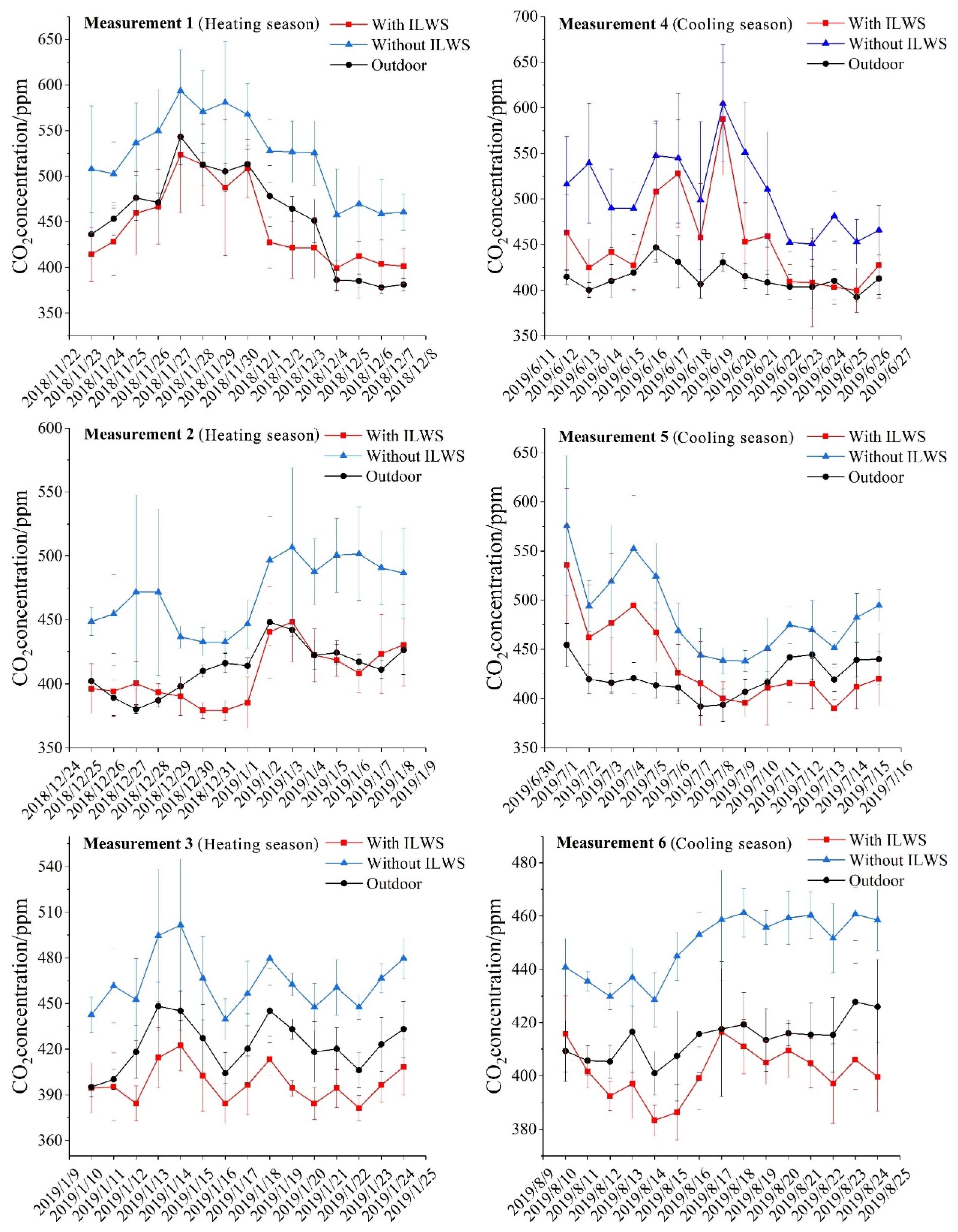
3.1. Comparison of CO₂ Concentration with and without ILWS

The daily average value of CO₂ concentration is shown in Figure 6. The outdoor CO₂ concentration fluctuates from 380 ppm to 450 ppm most of the time. However, in some scenarios, for example in measurement 1 in the heating season, it can even reach 550 ppm. It can be found that the CO₂ concentration at the west corridor (with ILWS) is lower than that of the east corridor (without ILWS), and sometimes it is even lower than the outdoor value. Specifically, as shown in

Table 6. Comparisons on indoor CO₂ concentration between the corridors.

Measurements	Average CO2 (ppm)			Difference	MRE	t-test Sig.	95% Confidence Interval of the Difference
	With ILWS $(C_W)$	Without ILWS $(C_E)$	$\mathrm{Outdoor} (C_S)$	$C_E-C_W$	$(C_E-C_W$$)/C_E$	$C_W\&C_E$	Lower	Upper
Measurement 1	445.8	522.3	455.7	76.5	17%	0.000	−12.91	−10.52
Measurement 2	407.4	471.0	412.6	63.6	16%	0.060	−0.03	1.51
Measurement 3	397.8	464.0	422.5	66.2	17%	0.039	0.02	1.01
Measurement 4	453.2	506.3	413.8	53.1	12%	0.000	12.08	15.03
Measurement 5	435.9	485.2	422.1	49.3	11%	0.000	16.90	19.17
Measurement 6	401.7	449.0	414.1	47.3	12%	0.000	18.55	19.16

Duration of the dataset: Measurement 1: 23 November 2018–7 December 2018; Measurement 2: 25 December 2018–8 January 2019; Measurement 3: 10 January 2019–24 January 2019; Measurement 4: 12 June 2019–26 June 2019; Measurement 5: 1 July 2019–15 July 2019; Measurement 6: 10 August 2019–24 August 2019.

, in the corridor using ILWS during the heating season, the CO₂ concentrations of measurement 1, measurement 2, and measurement 3 are 76.5 ppm, 63.6 ppm, and 66.2 ppm lower than those without ILWS. In the cooling season, the remaining three measured concentrations are 53.1 ppm, 49.3 ppm, and 47.3 ppm lower, respectively. Moreover, according to an independent sample t-test on $C_W \mathrm{and} C_E$ (with ILWS and without ILWS), the difference is statistically significant in most of the cases. Since the differences in air change rate and the number of people passing through the two corridors are not statistically significant (considered as equal), and there are no other objects that generate or absorb CO₂, the difference in CO₂ concentration in the two corridors were considered to be caused by the presence of ILWS. On average, the CO₂ concentration decreased by 16.7% in the heating season and 11.7% in the cooling season, respectively.

3.2. Comparison of Particulate Matter Concentration with and without ILWS

The daily average value in PM_0.3–1, PM_1–2.5, and PM_2.5–10 concentration is shown in Figure 7, Figure 8 and Figure 9. In all cases, the PMs concentrations are much higher in the heating season than in the cooling season. This trend is consistent with the national historical data [44,45]. The reasons for this trend are complicated. The main attributes that influence the concentration of PM are pollution source emissions and meteorological conditions. Coal-fired heating and incomplete combustion in vehicle engines at low temperatures may increase emissions in the heating season. The temperature inversion effect and less precipitation in the heating season may also become adverse meteorological conditions for pollutants’ diffusion and washout [46,47,48,49].

Figure 7 shows that the outdoor PM_0.3–1 concentration varies from 20–80 μg/m³ in the heating season and from 5–45 μg/m³ in the cooling season. By comparison, the PM_0.3–1 in the corridor without ILWS is much higher. The maximum value reaches 120 μg/m³ in the heating season and 55 μg/m³ in the cooling season. In the case of the ILWS, the value is in-between. Figure 8 shows outdoor PM_1–2.5 ranges from 30–180 μg/m³ in the heating season, 10–70 μg/m³ in the cooling season. The maximum value in the cases without ILWS reaches 225 μg/m³ in winter. Even in the cooling season, the maximum value can be as high as 85 μg/m³. The same thing goes for PM_2.5–10 (Figure 9). Outdoor PM_2.5–10 fluctuates from 40–220 μg/m³ in the heating season, 10–85 μg/m³ in the cooling season. Without ILWS, the maximum value breakthroughs 260 μg/m³ in the heating season and nearly 100 μg/m³ in the cooling season.

The results are summarized in

Table 7. Comparison of PMs concentration between the corridors.

Parameter	Measurements	Average PM0.3–1 (μg/m3)			Difference (μg/m3)	MRE	t-Test Sig.	95% Confidence Interval of the Difference
PM0.3–1		With ILWS $(C_W)$	Without ILWS $(C_E)$	Outdoor $(C_S)$	$C_E-C_W$	$(C_E-C_W$$)/C_E$	$C_W\&C_E$	Lower	Upper
	Measurement 1	60.9	72.0	58.8	11.1	15%	0.000	−9.62	−8.35
	Measurement 2	48.4	55.0	46.8	6.6	12%	0.000	−6.50	−5.63
	Measurement 3	56.6	67.1	58.9	10.5	16%	0.000	−11.56	−10.62
	Measurement 4	36.0	36.1	31.1	0.1	0.3%	0.189	−0.41	0.080
	Measurement 5	34.2	34.8	30.1	0.6	2%	0.000	−0.80	−0.44
	Measurement 6	24.2	25.4	22.3	1.2	5%	0.000	−1.38	−0.98
PM1–2.5
	Measurement 1	107.3	125.3	111.6	18	14%	0.000	−13.84	−11.44
	Measurement 2	83.5	92.3	82.4	8.8	10%	0.000	−8.74	−7.06
	Measurement 3	107.5	119.8	109.3	12.3	10%	0.000	−16.19	−14.20
	Measurement 4	53.2	58.0	50.7	4.8	8%	0.000	−5.03	−4.23
	Measurement 5	50.6	56.0	49.7	5.4	10%	0.000	−5.72	−5.12
	Measurement 6	33.3	38.4	33.2	5.1	13%	0.000	−5.39	−4.78
PM2.5–10
	Measurement 1	133.2	143.9	133.3	10.7	7%	0.000	−5.97	−3.06
	Measurement 2	103.8	109.1	100.3	5.3	5%	0.000	−5.82	−3.85
	Measurement 3	140.9	143.6	134.3	2.7	2%	0.000	−8.84	−6.38
	Measurement 4	65.2	70.1	60.4	4.9	7%	0.000	−5.60	−4.69
	Measurement 5	62.4	69.0	59.6	6.6	10%	0.000	−7.00	−6.28
	Measurement 5	39.7	46.0	37.8	6.3	14%	0.000	−6.75	−5.96

Duration of the dataset: Measurement 1: 23 November 2018–7 December 2018; Measurement 2: 25 December 2018–8 January 2019; Measurement 3: 10 January 2019–24 January 2019; Measurement 4: 12 June 2019–26 June 2019; Measurement 5: 1 July 2019–15 July 2019; Measurement 6: 10 August 2019–24 August 2019.

. The results from the independent sample t-test indicate that the differences in these groups are statistically significant in all the cases. During the three monitored periods in the heating season, the average PM_0.3–1 concentration in the corridor with ILWS is 11.1 μg/m³, 6.6 μg/m³, and 10.5 μg/m³ respectively (measurement 1–3) lower than that without ILWS. In the cooling season, the average PM_0.3–1 concentration with ILWS is 0.1 μg/m³, 0.6 μg/m³, and 1.2 μg/m³ respectively (measurement 4–6) lower than that without ILWS (Table 7, PM_0.3–1). During the three monitored periods in the heating season, the average PM_1–2.5 concentration in the corridor with ILWS is 18 μg/m³, 8.8 μg/m³, and 12.3 μg/m³ respectively (measurement 1–3) lower than that without ILWS. In the cooling season, the average PM_1–2.5 concentration with ILWS is 4.8 μg/m³, 5.4 μg/m³, and 5.1 μg/m³ respectively (measurement 4–6) lower than that without ILWS (Table 7, PM_1–2.5). During the three monitored periods in the heating season, the average PM_2.5–10 concentration in the corridor with ILWS is 10.7 μg/m³, 5.3 μg/m³, and 2.9 μg/m³ respectively (measurement 1–3) lower than that without ILWS. In the cooling season, the average PM_2.5–10 concentration with ILWS is 4.9 μg/m³, 6.6 μg/m³, and 6.3 μg/m³ respectively (measurement 4–6) lower than that without ILWS (Table 7, PM_2.5–10).

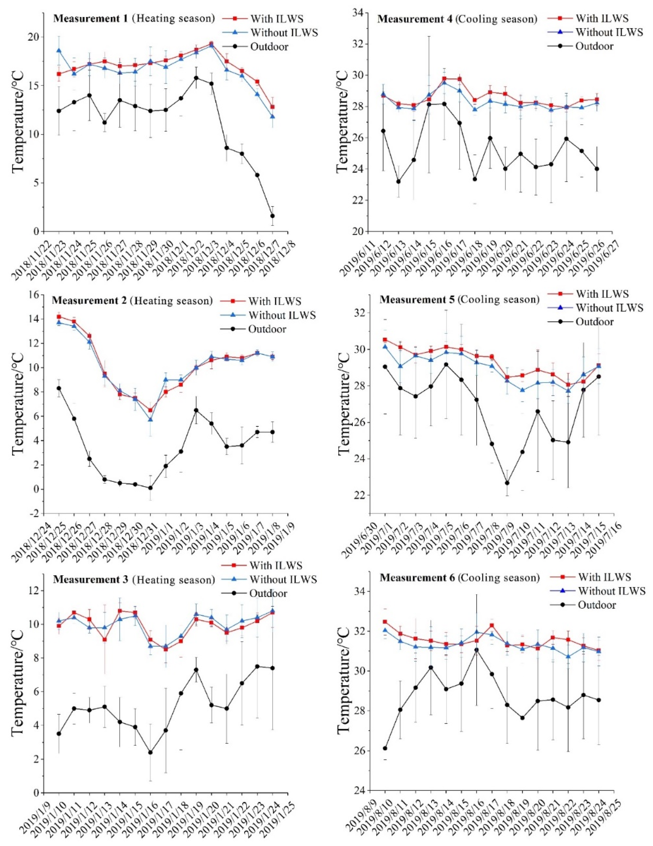
3.3. Comparison of Indoor Air Temperature with and without ILWS

During the experimental period, the average indoor air temperature is approximately 12.3 °C with the relative humidity of 54% in the heating season whereas the mean indoor temperature reaches about 30.0 °C with the relative humidity of 65% in the cooling season.

As shown in Figure 10, the outdoor temperature fluctuates sharply, while the indoor temperature is relatively stable. The temperature difference between indoor and outdoor is 3–6 °C, but the temperature difference between corridors with or without ILWS is much smaller. Data analysis (in

Table 8. Comparisons on air temperature between the corridors.

Season	Measurements	Average Temperature (°C)			Difference (°C)	MRE	t-Test Sig.	95% Confidence Interval of the Difference
		With ILWS $(C_W)$	Without ILWS $(C_E)$	Outdoor $(C_S)$	$C_E-C_W$	$(C_E-C_W$$)/C_E$	$C_W\&C_E$	Lower	Upper
Heating season	Measurement 1	17.0	16.6	11.4	−0.4	−2.4%	0.000	0.45	0.51
	Measurement 2	10.2	10.1	4.5	−0.1	−1.0%	0.890	−0.04	0.05
	Measurement 3	9.9	10.0	5.2	0.1	1.0%	0.000	0.03	0.07
Cooling season	Measurement 4	28.6	28.3	25.3	−0.3	−1.2%	0.000	0.27	0.30
	Measurement 5	29.3	28.9	26.8	−0.4	−1.4%	0.000	0.41	0.45
	Measurement 6	31.6	31.3	28.8	−0.3	−1.0%	0.000	0.21	0.24

Duration of the dataset: Measurement 1: 23 November 2018–7 December 2018; Measurement 2: 25 December 2018–8 January 2019; Measurement 3: 10 January 2019–24 January 2019; Measurement 4: 12 June 2019–26 June 2019; Measurement 5: 1 July 2019–15 July 2019; Measurement 6: 10 August 2019–24 August 2019.

) shows that in most of the cases, the difference in air temperature between the corridors with and without ILWS is statistically significant. The average air temperature in the corridor with ILWS is 0.13 °C higher than that without ILWS in the heating season, and 0.33 °C higher in the cooling season. Given the accuracy of the experimental instrument ($\pm 0.2$ °C), the ILWS just has a quite limited effect on indoor air temperature. However, further research is needed to rectify its effect on indoor air temperature.

3.4. Comparison of Indoor Relative Humidity with and without ILWS

The daily average relative humidity is plotted in Figure 11. It can be seen that in most of the days, whether in the heating season or in the cooling season, outdoor relative humidity is 10–30% higher than indoors. Relative humidity in the cases with the ILWS is slightly higher than that without ILWS. The data in

Table 9. Comparisons on relative humidity between the corridors.

Season	Measurements	Average Relative Humidity (%)			Difference	MRE	t-Test Sig.	95% Confidence Interval of the Difference
		With ILWS $(C_W)$	Without ILWS $(C_E)$	Outdoor $(C_S)$	$C_E-C_W$	$(C_E-C_W$$)/C_E$	$C_W\&C_E$	Lower	Upper
Heating season	Measurement 1	63.5	61.5	73.4	−2.0	−3.3%	0.000	2.40	2.65
	Measurement 2	54.2	52.3	69.1	−3.9	−7.5%	0.000	3.80	4.25
	Measurement 3	57.1	52.7	71.0	−4.4	−8.3%	0.000	3.01	3.30
Cooling season	Measurement 4	63.5	61.3	71.6	−1.9	−3.1%	0.000	2.07	2.34
	Measurement 5	67.6	65.9	75.2	−1.7	−2.6%	0.000	1.44	1.65
	Measurement 6	63.2	61.0	67.5	−2.2	−3.6%	0.000	2.15	2.38

Duration of the dataset: Measurement 1: 23 November 2018–7 December 2018; Measurement 2: 25 December 2018–8 January 2019; Measurement 3: 10 January 2019–24 January 2019; Measurement 4: 12 June 2019–26 June 2019; Measurement 5: 1 July 2019–15 July 2019; Measurement 6: 10 August 2019–24 August 2019.

show that in the three monitored periods in the heating season, the average relative humidity in the corridor with ILWS is 3.3%, 7.5%, and 8.3% higher than that without ILWS (6.4% higher on average). In the cooling season, the values are 3.1%, 2.6%, and 3.6% higher (3.1% higher on average). The increase in relative humidity should be related to the transpiration of plants.

4. Discussions

In this study, the method of field monitoring was adopted. Since the confounding variables were not perfectly controlled, the causal relationship between the living wall system and indoor air quality cannot be directly revealed. However, through the monitoring of the actual environment and statistical analysis of the data, it has been found that there are statistically significant differences in the CO₂ concentration, PM concentration, and relative humidity between the corridors with and without ILWS. However, since the form of the two corridors are the same, and the difference in air change rate, as well as intensity of use, between the two corridors, were not statistically significant, it can be inferred that the differences were caused by the ILWS. Indoor CO₂ and PMs concentration reduced, while temperature and relative humidity slightly increased. Results from this study were compared with other studies (

Table 10. Results comparisons with other studies.

Reference	Köppen Climatic Zone	Area of ILWS (m2)	Function & Volume of Space (m3)	Impact on CO2 Concentration (μg/m3/%)	Impact on PMs Concentration (μg/m3/%)	Impact on Temperature (°C/%)	Impact on Relative Humidity
This study	Cfa	10.6	Corridor 30.6	49.9–68.8↓ 12–17%↓	PM0.3–1: 1.9–9.4↓ 2.4–14.3%↓ PM1–2.5: 5.1–13.3↓ 10.3–11.3%↓ PM2.5–10: 5.9–6.2↓ 4.7–10.3%↓	0.1–0.4↑ 1–2.4%↑	3.1–6.4%↑
Ghazalli et al. [39]	Cfa	3.2	Corridor 27	Not tested	PM2.5: 48.5%↓ PM10: 82.6%↓ >PM10: 65.5%↓	→	2–3%↑
Su and Lin [40]	Cfa	5.72	Laboratory 38.88	21.3%↓	Not tested	2.5 °C↓ 11% ↓	2–4%↑
Gunawardena et al. [50]	Cfb	91	Atrium Not mentioned	Not tested	Not tested	0.2–0.7 °C↑ 1–3.1%↑	2.3–2.4%↑
Tudiwer et al. [42]	Cfb	5.5	Classroom 202	3.5%↓	Not tested	→	25.5%↑
Urrestarazu et al. [51]	Csa	8	Main hall 351	Not tested	Not tested	0.8–4.8 °C↓ 2.6–19.6%↓	6–21.3%↑
Rafael et al. [52]	Csa	7.74	Hall 195.4	Not tested	Not tested	4 °C↑	15%↑
Poorova et al. [53]	Dfb	3	Classroom 207.2	127.9↓ 14%↓	Not tested	1.7 °C↓ 4.6%↓	1.4%↑
Shao et al. [54]	Cfa	6.86	Office 88.92	25.7%–34.3%↓	Not tested	Not tested	Not tested

Note: ↑: increase; ↓: decrease; →: no significant change.

). Currently, the number of studies on ILWS is quite small, and the most studied climatic zone is Cfa in the Köppen classification. The impact of ILWS on CO₂ concentration reduction has been confirmed in studies, although the performance varies from case to case. Only two studies (this study and [39]), within the same climatic zone and similar space volume, investigated the impact of ILWS on PMs. Qualitatively, they draw the same conclusion that ILWS could reduce PMs concentration. However, quantitatively, the discrepancies in effectiveness are quite large. The influence of ILWS on temperature shows no obvious trend. In all the studies, relative humidity increases with the presence of ILWS. The increase in dry climatic zones is greater than that in humid regions.

The results from this study could be used as a reference for other research and development in a similar climatic zone. In this study, the ILWS was considered as a whole system to influence the monitored environmental parameters, which provided an understanding of the overall effect of a typical ILWS in the particular climatic zone, although the weight of each attribute within the system was still unknown. For example, as the results indicated that there was a statistically significant reduction in PMs caused by the presence of the ILWS, the main attributes could not be quantitatively or even qualitatively identified. Whether the pollutants were adsorbed by the plants’ leaves or by the water in the growing pods or by the water vapor produced by plants’ transpiration could not be separated out and given weight. In order to figure out the causal relationship, a number of strictly controlled experiments in sealed chambers are needed. Of course, this is very time-consuming. However, from the perspective of the built environment, more attention should be paid to the overall performance of a typical system to evaluate its effectiveness and feasibility. In addition, studying the overall impact could achieve even more accurate prediction results than studying the effects of individual attributes and then adding them up. Since, under real-world conditions, it is almost impossible to control all influencing factors, extract the weight of each one from a whole system, and eliminate the possibility of mutual influence between attributes. Real-world tests can be used as references for other projects or studies, where an analogy method could be used with a large database to predict the potential impact of a new ILWS. A number of tests of different ILWS projects from different climatic zones with different combinations of plants are needed to build such a database. When an analogy method is used, the higher the matching degree of parameters, the higher the accuracy of prediction results will be. Area of ILWS to space volume ratio could be used as a key parameter for such an analogy evaluation, along with other parameters, such as plant type, the proportion of plants’ combination, daily PAR on the ILWS, and so forth. In order to match the parameters from a new ILWS to those from a database, a training sample dataset is needed for machine learning, using a computer algorithm to determine the weight of each parameter. This study is just the first step, as one of the important case studies in many, towards this target.

The idea of introducing ILWS to the indoor environment starts from improving indoor air quality and environmental aesthetic value for human well-being [33]. However, the benefits do not stop here. The potential of using ILWS to reduce building energy consumption in heating and cooling seasons cannot be ignored [28]. The direct impact of ILWS on indoor air temperature is still inconclusive. It may be also influenced by some exterior factors, such as the orientation of the building, the location of openings on the building, or even the function of space. Further studies on these factors are needed. The indirect effect of ILWS on building energy saving could be mainly reflected in ventilation energy consumption. Currently, the main method of removing indoor air pollutants still relies on diluting the indoor pollutants by ventilating the fresh air from the outside [55]. During the spring or autumn seasons, when the outside temperature fluctuates within the temperature comfort zone, usually 18–26 °C, natural ventilation can be used directly [56]. However, in cooling or heating seasons when the temperature is beyond the comfort zone, the fresh air needs to be pre-heated or pre-cooled before it is ventilated mechanically to the indoor space in order to reach the indoor designed temperature. Therefore, in such scenarios, the ventilation rate, determined by the fresh air requirement, has a proportional relationship with the building energy consumption in ventilating sector. Introducing ILWS into buildings may improve the air quality, thus equivalently reduces the fresh air requirement and the ventilation rate when the outside temperature is beyond the comfort zone for natural ventilation. Apart from indoor and outdoor temperature and humidity differences, the performance of energy consumption reduction in ventilation is mainly determined by the CO₂ absorption rate of ILWS instead of the adsorption rate of PMs or VOC. It is because PMs and VOC can be adsorbed by various artificial porous materials, but there is currently no low-cost practical method for massive CO₂ conversion [57]. Plants’ photosynthesis is still the most extensive process of carbon dioxide to oxygen conversion on earth. Consequently, if working with other artificial filters, ILWS may reduce the building energy consumption through ventilation heat loss/gain in heating or cooling seasons. The effectiveness of this mechanism still needs further study.

5. Conclusions

In this study, a field monitoring test of the ILWS was implemented in order to evaluate the system performance for the Cfa climate zone (Köppen climate classification) from November 2018 to August 2019. The influences of the ILWS on indoor air quality with and without ILWS between two parallel corridors were studied in an office building based on different parameters such as CO₂ concentration, PM, atmospheric temperature, and relative humidity. Some key findings are concluded as follows:

• ILWS could be a promising opportunity in the eco-design of the buildings considering its aesthetic value and purification function of indoor air.
• Based on the results from the statistical analysis, the differences in CO₂ and PM concentration in the two corridors are statistically significant—this indicates the positive effect of ILWS on improving indoor air quality.
• In terms of the CO₂ concentration, the average indoor air temperature of the corridors with ILWS can be reduced to the same level of outdoor condition, or even slightly lower than outdoor levels.
• The purification performance of CO₂ and PMs in the heating season is better in comparison with that in the cooling season due to the local seasonal climate condition and pollutant emission.
• The effect of ILWS on indoor air temperature is quite limited. However, the relative humidity in the corridor with ILWS is slightly higher (3.1–6.4%) than that without ILWS.

References

1. Wilson, T. Population Growth. In International Encyclopedia of Human Geography, 2nd ed.; Kobayashi, A., Ed.; Elsevier: Oxford, UK, 2020; pp. 1–6. [Google Scholar]
2. Liu, C.H.; Rosenthal, S.S.; Strange, W.C. The vertical city: Rent gradients, spatial structure, and agglomeration economies. J. Urban Econ. 2018, 106, 101–122. [Google Scholar] [CrossRef]
3. Bek, M.A.; Azmy, N.; Elkafrawy, S. The effect of unplanned growth of urban areas on heat island phenomena. Ain Shams Eng. J. 2018, 9, 3169–3177. [Google Scholar] [CrossRef]
4. von Schneidemesser, E.; Steinmar, K.; Weatherhead, E.C.; Bonn, B.; Gerwig, H.; Quedenau, J. Air pollution at human scales in an urban environment: Impact of local environment and vehicles on particle number concentrations. Sci. Total Environ. 2019, 688, 691–700. [Google Scholar] [CrossRef] [PubMed]
5. Vieira, J.; Matos, P.; Mexia, T.; Silva, P.; Lopes, N.; Freitas, C.; Correia, O.; Santos-Reis, M.; Branquinho, C.; Pinho, P. Green spaces are not all the same for the provision of air purification and climate regulation services: The case of urban parks. Environ. Res. 2018, 160, 306–313. [Google Scholar] [CrossRef] [PubMed]
6. Cai, M.; Xin, Z.; Yu, X. Particulate matter transported from urban greening plants during precipitation events in Beijing, China. Environ. Pollut. 2019, 252, 1648–1658. [Google Scholar] [CrossRef]
7. Deng, S.; Ma, J.; Zhang, L.; Jia, Z.; Ma, L. Microclimate simulation and model optimization of the effect of roadway green space on atmospheric particulate matter. Environ. Pollut. 2019, 246, 932–944. [Google Scholar] [CrossRef]
8. Charoenkit, S.; Yiemwattana, S. Living walls and their contribution to improved thermal comfort and carbon emission reduction: A review. Build. Environ. 2016, 105, 82–94. [Google Scholar] [CrossRef]
9. Marchi, M.; Pulselli, R.M.; Marchettini, N.; Pulselli, F.M.; Bastianoni, S. Carbon dioxide sequestration model of a vertical greenery system. Ecol. Model. 2015, 306, 46–56. [Google Scholar] [CrossRef]
10. Klingberg, J.; Broberg, M.; Strandberg, B.; Thorsson, P.; Pleijel, H. Influence of urban vegetation on air pollution and noise exposure–A case study in Gothenburg, Sweden. Sci. Total Environ. 2017, 599–600, 1728–1739. [Google Scholar] [CrossRef]
11. Lacasta, A.M.; Penaranda, A.; Cantalapiedra, I.R.; Auguet, C.; Bures, S.; Urrestarazu, M. Acoustic evaluation of modular greenery noise barriers. Urban Urban Green. 2016, 20, 172–179. [Google Scholar] [CrossRef] [Green Version]
12. Van Renterghem, T.; Forssén, J.; Attenborough, K.; Jean, P.; Defrance, J.; Hornikx, M.; Kang, J. Using natural means to reduce surface transport noise during propagation outdoors. Appl. Acoust. 2015, 92, 86–101. [Google Scholar] [CrossRef] [Green Version]
13. Madre, F.; Clergeau, P.; Machon, N.; Vergnes, A. Building biodiversity: Vegetated façades as habitats for spider and beetle assemblages. Glob. Ecol. Conserv. 2015, 3, 222–233. [Google Scholar] [CrossRef] [Green Version]
14. Oh, R.R.Y.; Richards, D.R.; Yee, A.T.K. Community-driven skyrise greenery in a dense tropical city provides biodiversity and ecosystem service benefits. Landsc. Urban Plan. 2018, 169, 115–123. [Google Scholar] [CrossRef]
15. Mayrand, F.; Clergeau, P.; Vergnes, A.; Madre, F. Chapter 3.13–Vertical Greening Systems as Habitat for Biodiversity. In Nature Based Strategies for Urban and Building Sustainability; Pérez, G., Perini, K., Eds.; Butterworth-Heinemann: Oxford, UK, 2018; pp. 227–237. [Google Scholar]
16. Dahanayake, K.W.D.K.; Chow, C.L. Studying the potential of energy saving through vertical greenery systems: Using EnergyPlus simulation program. Energy Build. 2017, 138, 47–59. [Google Scholar] [CrossRef]
17. Poddar, S.; Park, D.Y.; Chang, S. Simulation Based Analysis on the Energy Conservation Effect of Green Wall Installation for Different Building Types in a Campus. Energy Procedia 2017, 111, 226–234. [Google Scholar] [CrossRef]
18. Morakinyo, T.E.; Lau, K.K.; Ren, C.; Ng, E. Performance of Hong Kong’s common trees species for outdoor temperature regulation, thermal comfort and energy saving. Build. Environ. 2018, 137, 157–170. [Google Scholar] [CrossRef]
19. Coma, J.; Pérez, G.; de Gracia, A.; Burés, S.; Urrestarazu, M.; Cabeza, L.F. Vertical greenery systems for energy savings in buildings: A comparative study between green walls and green facades. Build. Environ. 2017, 111, 228–237. [Google Scholar] [CrossRef] [Green Version]
20. Yaghoobian, N.; Srebric, J. Influence of plant coverage on the total green roof energy balance and building energy consumption. Energy Build. 2015, 103, 1–13. [Google Scholar] [CrossRef] [Green Version]
21. Lee, L.S.H.; Jim, C.Y. Energy benefits of green-wall shading based on novel-accurate apportionment of short-wave radiation components. Appl. Energy 2019, 238, 1506–1518. [Google Scholar] [CrossRef]
22. Zazzini, P.; Grifa, G. Energy Performance Improvements in Historic Buildings by Application of Green Walls: Numerical Analysis of an Italian Case Study. Energy Procedia 2018, 148, 1143–1150. [Google Scholar] [CrossRef]
23. Cui, Y.; Zheng, H. Impact of Three-Dimensional Greening of Buildings in Cold Regions in China on Urban Cooling Effect. Procedia Eng. 2016, 169, 297–302. [Google Scholar] [CrossRef]
24. Ávila-Hernández, A.; Simá, E.; Xamán, J.; Hernández-Pérez, I.; Téllez-Velázquez, E.; Chagolla-Aranda, M.A. Test box experiment and simulations of a green-roof: Thermal and energy performance of a residential building standard for Mexico. Energy Build. 2020, 209, 109709. [Google Scholar] [CrossRef]
25. Coma, J.; Chàfer, M.; Pérez, G.; Cabeza, L.F. How internal heat loads of buildings affect the effectiveness of vertical greenery systems? An experimental study. Renew. Energy 2019, 151, 919–930. [Google Scholar] [CrossRef]
26. Bustami, R.A.; Belusko, M.; Ward, J.; Beecham, S. Vertical greenery systems: A systematic review of research trends. Build. Environ. 2018, 146, 226–237. [Google Scholar] [CrossRef]
27. Veisten, K.; Smyrnova, Y.; Kl Boe, R.; Hornikx, M.; Mosslemi, M.; Kang, J. Valuation of Green Walls and Green Roofs as Soundscape Measures: Including Monetised Amenity Values Together with Noise-attenuation Values in a Cost-benefit Analysis of a Green Wall Affecting Courtyards. Int. J. Environ. Res. Public Health 2012, 9, 3770–3788. [Google Scholar] [CrossRef] [Green Version]
28. Safikhani, T.; Abdullah, A.M.; Ossen, D.R.; Baharvand, M. Thermal Impacts of Vertical Greenery Systems. Environ. Clim. Technol. 2014, 14, 5. [Google Scholar] [CrossRef] [Green Version]
29. Kingsbury, N. Planting Green Roofs and Living Walls; Timber Press: Portland, OR, USA, 2008. [Google Scholar]
30. Cameron, R.W.F.; Taylor, J.E.; Emmett, M.R. What’s ‘cool’ in the world of green façades? How plant choice influences the cooling properties of green walls. Build. Environ. 2014, 73, 198–207. [Google Scholar] [CrossRef] [Green Version]
31. Mårtensson, L.L.; Wuolo, A.A.; Fransson, A.A.; Emilsson, T.T. Plant performance in living wall systems in the Scandinavian climate. Ecol. Eng. 2014, 71, 610–614. [Google Scholar] [CrossRef] [Green Version]
32. Gunawardena, K.; Steemers, K. Living walls in indoor environments. Build. Environ. 2019, 148, 478–487. [Google Scholar] [CrossRef]
33. López-Aparicio, S.; Smolík, J.; Mašková, L.; Součková, M.; Grøntoft, T.; Ondráčková, L.; Stankiewicz, J. Relationship of indoor and outdoor air pollutants in a naturally ventilated historical building envelope. Build. Environ. 2011, 46, 1460–1468. [Google Scholar] [CrossRef]
34. Pettit, T.; Irga, P.J.; Torpy, F.R. Towards practical indoor air phytoremediation: A review. Chemosphere 2018, 208, 960–974. [Google Scholar] [CrossRef]
35. Jafari, M.J. Association of Sick Building Syndrome with Indoor Air Parameters. Tanaffos 2015, 14, 55–62. [Google Scholar]
36. Myhrvold, A.; Olesen, E. Pupil’s Health and Performance due to Renovation of Schools. In Proceedings of the Healthy Buildings/IAQ, Washington, DC, USA, 27 September–2 October 1997; Volume 1, pp. 81–86. [Google Scholar]
37. Dzierzanowski, K.; Popek, R.; Gawrońska, H.; Saebø, A.; Gawroński, S.W. Deposition of particulate matter of different size fractions on leaf surfaces and in waxes of urban forest species. Int. J. Phytoremediation 2011, 13, 1037–1046. [Google Scholar] [CrossRef]
38. El Hamdani, S.; Limam, K.; Abadie, M.O.; Bendou, A. Deposition of fine particles on building internal surfaces. Atmos. Environ. 2008, 42, 8893–8901. [Google Scholar] [CrossRef]
39. Ghazalli, A.J.; Brack, C.; Bai, X.; Said, I. Alterations in use of space, air quality, temperature and humidity by the presence of vertical greenery system in a building corridor. Urban Urban Green. 2018, 32, 177–184. [Google Scholar] [CrossRef]
40. Su, Y.; Lin, C. Removal of Indoor Carbon Dioxide and Formaldehyde Using Green Walls by Bird Nest Fern. Hortic. J. 2015, 84, 69–76. [Google Scholar] [CrossRef] [Green Version]
41. Torpy, F.R.; Zavattaro, M.; Irga, P.J. Green wall technology for the phytoremediation of indoor air: A system for the reduction of high CO2 concentrations. Air Qual. Atmos. Health 2016, 10, 1–11. [Google Scholar] [CrossRef]
42. Tudiwer, D.; Korjenic, A. The effect of an indoor living wall system on humidity, mould spores and CO2 concentration. Energy Build. 2017, 146, 73–86. [Google Scholar] [CrossRef]
43. National Meteorological Science Data Center. National meteorological Observation Data. Available online: http://data.cma.cn/data/online/t/1 (accessed on 5 January 2020).
44. Li, J.; Liao, H.; Hu, J.; Li, N. Severe particulate pollution days in China during 2013–2018 and the associated typical weather patterns in Beijing-Tianjin-Hebei and the Yangtze River Delta regions. Environ. Pollut. 2019, 248, 74–81. [Google Scholar] [CrossRef]
45. Zhang, Y.; Cao, F. Fine particulate matter (PM2.5) in China at a city level. Sci. Rep. 2015, 5, 1–12. [Google Scholar] [CrossRef] [PubMed] [Green Version]
46. Bollasina, M.A.; Ming, Y.; Ramaswamy, V. Anthropogenic Aerosols and the Weakening of the South Asian Summer Monsoon. Sci. Am. Assoc. Adv. Sci. 2011, 334, 502–505. [Google Scholar] [CrossRef] [PubMed] [Green Version]
47. Yin, Z.; Wang, H. Seasonal prediction of winter haze days in the north central North China Plain. Atmos. Chem. Phys. 2016, 16, 14843–14852. [Google Scholar] [CrossRef] [Green Version]
48. Cheng, X.; Zhao, T.; Gong, S.; Xu, X.; Han, Y.; Yin, Y.; Tang, L.; He, H.; He, J. Implications of East Asian summer and winter monsoons for interannual aerosol variations over central-eastern China. Atmos. Environ. 2016, 129, 218–228. [Google Scholar] [CrossRef]
49. Yin, X.; Sun, Z.; Miao, S.; Yan, Q.; Wang, Z.; Shi, G.; Li, Z.; Xu, W. Analysis of abrupt changes in the PM2.5 concentration in Beijing during the conversion period from the summer to winter half-year in 2006–2015. Atmos. Environ. 2019, 200, 319–328. [Google Scholar] [CrossRef]
50. Gunawardena, K.R.; Steemers, K. Living wall influence on microclimates: An indoor case study. J. Phys. Conf. Ser. 2019, 1343, 12188. [Google Scholar] [CrossRef]
51. Pérez-Urrestarazu, L.; Fernández-Cañero, R.; Franco, A.; Egea, G. Influence of an active living wall on indoor temperature and humidity conditions. Ecol. Eng. 2016, 90, 120–124. [Google Scholar] [CrossRef]
52. Fernández-Cañero, R.; Urrestarazu, L.P.; Franco Salas, A. Assessment of the Cooling Potential of an Indoor Living Wall using Different Substrates in a Warm Climate. Indoor Built. Environ. 2012, 21, 642–650. [Google Scholar] [CrossRef]
53. Poorova, Z.; Vranayova, Z. Humidity, Air Temperature, CO2 and Well-Being of People with and Without Green Wall; Springer International Publishing: Cham, Switzerland, 2020; pp. 336–346. [Google Scholar]
54. Shao, Y.; Li, J.; Zhou, Z.; Hu, Z.; Zhang, F.; Cui, Y.; Chen, H. The effects of vertical farming on indoor carbon dioxide concentration and fresh air energy consumption in office buildings. Build. Environ. 2021, 195, 107766. [Google Scholar] [CrossRef]
55. Ahmed, K.; Kurnitski, J.; Sormunen, P. Demand controlled ventilation indoor climate and energy performance in a high performance building with air flow rate controlled chilled beams. Energy Build. 2015, 109, 115–126. [Google Scholar] [CrossRef]
56. Zhang, F.; Haddad, S.; Nakisa, B.; Rastgoo, M.N.; Candido, C.; Tjondronegoro, D.; de Dear, R. The effects of higher temperature setpoints during summer on office workers’ cognitive load and thermal comfort. Build. Environ. 2017, 123, 176–188. [Google Scholar] [CrossRef] [Green Version]
57. Kim, M.K.; Choi, J. Can increased outdoor CO2 concentrations impact on the ventilation and energy in buildings? A case study in Shanghai, China. Atmos. Environ. 2019, 210, 220–230. [Google Scholar] [CrossRef]
Figure 1. Monthly temperature and relative humidity statistics.
Sustainability 13 07884 g001
Figure 2. Monitoring location: (A): location of the site; (B): floor plan and the setup of measuring devices (Unit in mm).
Sustainability 13 07884 g002
Figure 3. Photo and diagrams of the ILWS: (A): photo; (B): section; (C): PAR measuring points (Unit in mm).
Sustainability 13 07884 g003
Figure 4. Monitoring equipment: ((A): air quality monitor; (B): PAR meter; (C): anemometer; (D): passenger flow counter).
Sustainability 13 07884 g004
Figure 5. Average photosynthetic photon flux density (PPFD) under natural light and artificial light.
Sustainability 13 07884 g005
Figure 6. 15 days’ record on CO2 concentration.
Sustainability 13 07884 g006
Figure 7. 15 days’ record on PM0.3–1 concentration.
Sustainability 13 07884 g007
Figure 8. 15 days’ record on PM1–2.5 concentration.
Sustainability 13 07884 g008
Figure 9. 15 days’ record on PM2.5–10 concentration.
Sustainability 13 07884 g009
Figure 10. 15 days’ record on air temperature.
Sustainability 13 07884 g010
Figure 11. 15 days’ record on relative humidity.
Sustainability 13 07884 g011