Proton Exchange Membrane Fuel Cells Modeling Using Chaos Game Optimization Technique

Abstract

For the precise simulation performance, the accuracy of fuel cell modeling is important. Therefore, this paper presents a developed optimization method called Chaos Game Optimization Algorithm (CGO). The developed method provides the ability to accurately model the proton exchange membrane fuel cell (PEMFC). The accuracy of the model is tested by comparing the simulation results with the practical measurements of several standard PEMFCs such as Ballard Mark V, AVISTA SR-12.5 kW, and 6 kW of the Nedstack PS6 stacks. The complexity of the studied problem stems from the nonlinearity of the PEMFC polarization curve that leads to a nonlinear optimization problem, which must be solved to determine the seven PEMFC design variables. The objective function is formulated mathematically as the total error squared between the laboratory measured terminal voltage of PEMFC and the estimated terminal voltage yields from the simulation results using the developed model. The CGO is used to find the best way to fulfill the preset requirements of the objective function. The results of the simulation are tested under different temperature and pressure conditions. Moreover, the results of the proposed CGO simulations are compared with alternative optimization methods showing higher accuracy.

1. Introduction

In addition to the environmental impact of fossil fuels, they are declining and unsustainable sources of energy. For this reason, more focus has been given to develop clean renewable energy resources [1,2]. FCs are among promising energy resources. In FCs, electricity is generated by chemical reactions from chemical energy [3,4,5]. PEMFC is one of the FCs that have been widely used. The major characteristics and benefits of the PEMFCs are: (1) low operating pressure and temperature, (2) high performance ratio, and (3) no waste materials [6]. The fuel cell temperature requirements vary from 50 to 100 °C and the output power is between 30 and 60 percent under these temperature operating conditions [6,7]. In [8], a switched reluctance motor powered by the PEMFC’s stack is used to optimize the operating performance. The performance is examined in terms of: (1) torque-ampere ratio, (2) torque smoothness, and (3) starting torque. The work in [9] applies an algorithm to a step-up converter in order to improve the performance of PEMFCs. A comprehensive review of the benefits of different design and optimization algorithms for PEMFCs is provided in [10]. In [11], a model is introduced for the PEMFC to save the undesirable thermal energy generated during the operation. The model uses the unoccupied capacity of the PEMFC to produce/store hydrogen.

Many researchers have recently drawn attention to the construction of a PEMFC model. A hybrid optimization approach is introduced in [12] for estimating the parameters of the PEMFC. The analysis in this work is performed on a 250 W stack, NedStack PS6, BCS 500-W, and SR-12 PEM 500 W fuel cells. To obtain results which are very similar to experimental results, the researchers strive to find a trustworthy PEMFC model with software programs and modeling that reduce substantial time and effort [13]. The PEMFC modeling is an important and promising research field. Both conventional and metaheuristic methods can be used to extract the parameters of the fuel cell. For example, the work in [14] introduces an evaluation of parameters’ effects on the FC performance and model validation besides identification of optimal parameters. Taleb [15] presents monitoring of the operation of the PEMFC using a model-based approach. Experimental validation is done to the model using a frequency identification method. Then, time series identification is conducted using a least square method. In [16], a semi-empirical model is proposed based on the data of a three-cell SOFC stack, which predicts the performance of real stacks. The effects of key operation parameters were studied. The generalized reduced gradient technique is introduced in [17]. Moreover, in that context, a large number of complex analysis techniques were implemented to obtain an accurate fuel cell model [18,19,20].

Traditional optimization methods are unable to achieve sufficient results over a fair period. There are also drawbacks of traditional optimization methods which includes: (i) sensitivity for the initial problem estimate, (ii) reliance on solution exactness on the differential equation solver, and (iii) the possibility of getting trapped in a local solution. The probability of becoming trapped in a local optimal solution increases when dealing with highly nonlinear problems.

To efficiently deal with complex optimization problems, various algorithms have been developed. One of these algorithms is the CGO algorithm, which was introduced by Talatahari, Siamak, and Mahdi Azizi. [21]. The new optimization approach can be chosen to solve various problems in the field of engineering and other areas such as manufacturing applications and scientific models. The key idea of the CGO algorithm consists of some theories of chaos, which consider the construction of fractals according to the chaos game and the fractal problems of self-similarity. The findings have shown the superiority of the CGO in most cases. The theory of chaos shows that a few slight modifications in the initial guess of a complex system led to drastic variations in the conditions of these systems as they depend on the initial conditions.

In this paper, a new application of the CGO algorithm is presented to achieve the optimal PEMFC model design parameters. The objective of this study is to develop a PEMFC theoretical model. The results of the developed model are tested using measurements data provided by practical experiments. The experimentally measured data should yield close results to those found by the theoretical model. Considering that the data provided by the manufacturers are insufficient, and because of the nonlinear properties of the PEMFC as well as the seven design variables, the current–voltage characteristics of the PEMFC must be modeled. Thus, a NLOP is mathematically formulated in this study. In this formulated problem, the objective function is to achieve the minimum value of the square errors between the experimentally measured PEMFC voltage and the determined voltages by the developed model. The CGO algorithm is implemented explicitly to minimize the FF. The theoretical model’s simulation effects are also tested at different temperatures and pressures.

The contribution of this research study can be summarized as: (1) the static theoretical models of the different types of PEMFCs are introduced and the estimated output voltages of the PEMFCs are compared with the measured voltages to evaluate the adequateness of the model, and (2) the robustness of the proposed CGO algorithm in minimizing the objective function is verified by comparing the results with other optimization methods.

2. Modeling of The PEMFCS Methods

To explain PEMFC equations and to assess their simulation effectiveness, the model given by Mann et al. [22] is chosen. This model is often used as a reference for the research analysis in more than one literature paper. The number of series cells ($N_{cells}$) is expressed by (1) [22,23,24] in the mathematical equation of terminal voltage from the PEM fuel cell ($V_{stack}$).

$$V_{stack}=N_{cells}.\left(E_{nernst}-v_{act}-v_{\mathsf{\Omega }}-v_{conc}\right)$$

(1)

where $E_{nernst}$ is the Nernst voltage of a cell, $v_{act}$ is the overpotential of cell activation, $v_{\mathsf{\Omega }}$ is the ohmic voltage drop in the cell, and $v_{conc}$ is the over-potential of the concentration. If the temperature is below 100 °C, $E_{nernst}$ is calculated using Equation (2). The voltage drops $v_{act}, v_{\mathsf{\Omega }},$ and $v_{conc}$ can be calculated using (3)–(5), respectively [22,24].

$$E_{Nernst}=1.229-0.85\times {10}^{-3}\left(T_{fc}-298.15\right)+4.3085\times {10}^{-5}{T}_{fc}\ln \left(P_{H_2}\sqrt{P_{O_2}}\right)$$

(2)

$$v_{act}=-\left[{\xi }_1+{\xi }_2{T}_{fc}+{\xi }_3{T}_{fc}\ln \left(C_{O_2}\right)+{\xi }_4{T}_{fc}\ln \left(I_{fc}\right)\right]$$

(3)

$$E_{Nernst}=1.229-0.85\times {10}^{-3}\left(T_{fc}-298.15\right)+4.3085\times {10}^{-5}{T}_{fc}\ln \left(P_{H_2}\sqrt{P_{O_2}}\right)$$

(4)

$$E_{Nernst}=1.229-0.85\times {10}^{-3}\left(T_{fc}-298.15\right)+4.3085\times {10}^{-5}{T}_{fc}\ln \left(P_{H_2}\sqrt{P_{O_2}}\right)$$

(5)

$$v_{act}=-\left[{\xi }_1+{\xi }_2{T}_{fc}+{\xi }_3{T}_{fc}\ln \left(C_{O_2}\right)+{\xi }_4{T}_{fc}\ln \left(I_{fc}\right)\right]$$

(6)

where

$$C_{O_2}=\frac{P_{O_2}}{{\mathrm{5.08.10}}^6}. exp\left(498/T_{fc}\right)$$

(7)

$$v_{\mathsf{\Omega }}=I_{fc}\left(R_m+R_c\right); R_m=\frac{{\rho }_{m}l}{M_A}$$

(8)

where

$${\rho }_m=\frac{181.6\left[1+0.03\left(\frac{I_{fc}}{M_A}\right)+0.062{\left(\frac{I_{fc}}{303}\right)}^2{\left(\frac{I_{fc}}{M_A}\right)}^{2.5}\right]}{\left[\lambda -0.634-3\left(\frac{I_{fc}}{M_A}\right)\right].exp\left[4.18\left(\frac{T_{fc}-303}{T_{fc}}\right)\right]}$$

(9)

$$v_{conc}=-\beta .\ln \left(1-\frac{J}{J_{max}}\right)$$

(10)

where $T_{fc}$ represents the PEMFC temperature in Kelvin (K), $P_H$ and $P_O$ are the hydrogen (${\mathrm{H}}_2$) pressure and oxygen (${\mathrm{O}}_2$) pressure, respectively, ${\mathrm{I}}_{\mathrm{fc}}$ is the fuel cell current (A), $M_A$ is the membrane surface area (cm²), ${\mathrm{C}}_{{\mathrm{O}}_2}$ is the concentration of ${\mathrm{O}}_2$ (mol/cm³), ${\xi }_1-{\xi }_4$ are semi-empirical factors, $R_m$ denotes the membrane resistance (Ω), $R_c$ is the leads’ resistances (Ω), $\mathrm{l}$ is the membrane thickness (cm), ${\rho }_m$ denotes the membrane resistivity (Ω.cm), λ is a tunable design variable, $\mathsf{\beta }$ represents a constant of an empirical range, $J$ refers to the current density (A/cm²), and $J_{max}$ is the maximum current density (A/cm²).

${\xi }_1-{\xi }_4$ are design variables which are established according to the geometrical dimensioning and the material resources of the manufactured fuel cells [23]. The fact that the design variable λ is dependent on different factors such as relative humidity, the stoichiometric ratio, makes its design a complex task. Hence, in this paper, the value of λ is assumed to be varied from 13 to 23. As λ becomes less, this indicates higher cell relative humidity. On the other hand, as λ becomes greater, it is an indication of the supersaturated conditions [7,22,23]. $\beta$ is a design variable for Equation (5) which can be computed using Equation (6).

$$\beta =\frac{\Re .T_{fc}}{2\alpha F}$$

(11)

where $\Re$ is the ideal gas constant, F refers to the Faraday’s constant, and α is the charge transfer coefficient.

It can be noted from Equations (5) and (6) that the drop in the concentration voltage follows a linear relationship with the temperature and the current density.

There are seven design variables (i.e., ${\mathsf{\xi }}_1-{\mathsf{\xi }}_4$, λ, Rc, and β) to be determined when constructing the model for the PEM fuel cells to utilize it in any further electric power system investigations.

3. Problem Formulation

The problem introduced in this article is solved using the newly developed CGO algorithm. The PEMFC model introduces nonlinear characteristics including multiple unknown design variables due to a shortage in manufacturing data about PEMFCs. Therefore, a detailed model is a challenge that must be addressed. To achieve the unique, dependable model, there are seven design variables to be tuned. These variables must be accurately calculated in order to minimize the FF. The FF is the sum of the square of the errors which is the difference between the terminal voltage calculated from the PEMFC and the terminal voltage observed by measurements as provided in Equation (7) [21,23]. The proposed fitness function is minimized by using the CGO algorithm. The solution of the optimization problem yields the design value for the aforementioned design variables: ${\mathsf{\xi }}_1-{\mathsf{\xi }}_4$, λ, Rc, and β [25].

$$FF=\left(SSE\right)=\left({\displaystyle \sum }_{m=1}^{N_{samples}}{\left[V_{FC,exp}\left(m\right)-V_{FC,est}\left(m\right)\right]}^2\right)$$

(12)

where $N_{samples}$ refers to the number of the voltages measured, $m$ defines the iteration number, $V_{FC,exp}$ is the PEMFC measured voltage (V), and $V_{FC,est}$ is the PEMFC computed voltage by the introduced model (V).

4. The Chaos Game Optimization Algorithm

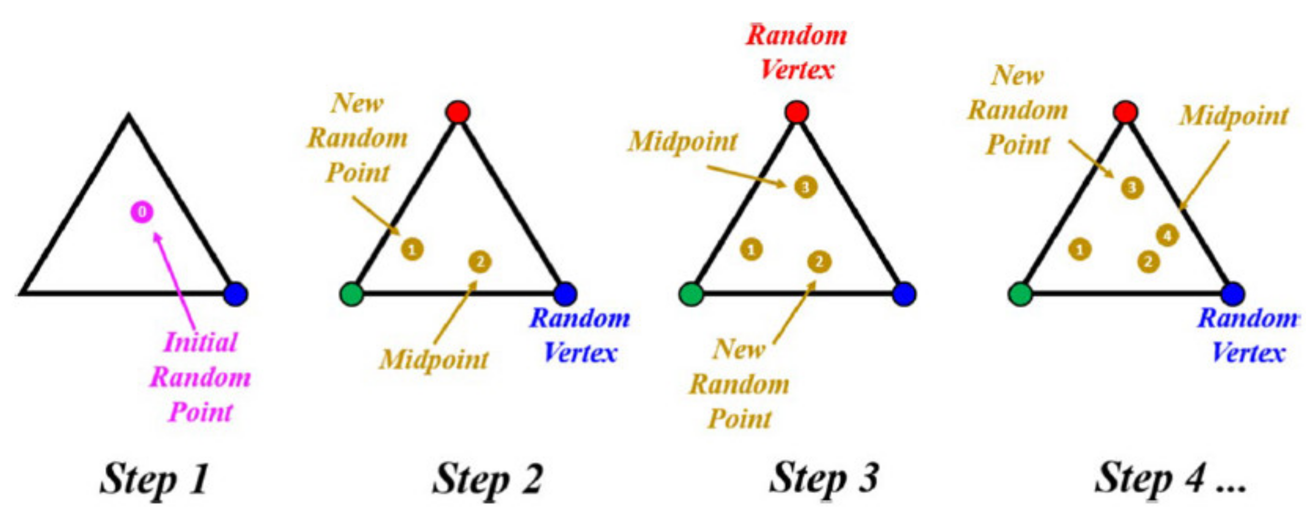
Studying the use of chaotic systems attracted many researchers as the theme of chaos achieves a high interdisciplinary level [26]. Employing the chaotic systems in the optimization algorithms is an example, a new metaheuristic Chaos Game Optimization is introduced. The CGO algorithm’s key concept is based on the chaos theory in which fractals are configured through the technique of the chaos game. The theory of chaos game is used as the key principle of the algorithm in the CGO method.

4.1. Inspiration

Chaos theory focuses on the basic characteristics of dynamically sensitive systems to the initial conditions. In view of the randomness of these complex processes, the principle of chaos refers to the presence of certain fundamental patterns.

The method of constructing fractals using the initial form and a random initial point is the Chaos Game. The main goal is to construct an iterative sequence of points to enter a sketch of similar form in various scales. Firstly, it is important to correctly place a triangle vertex. A random, initial point for the formation of fractal is chosen. The next item is then calculated as a part of the space between the first point and the random vertex. A fractal is generated while repeating this step with regard to the initial point and the vertex selected. Initially, the principal fractal form, which is triangular, is formed by three vertices. Dice with two, red, blue and green faces are used. The fractal, which is a seed, is chosen as a first random point. The first seed is pushed towards the corresponding vertex in the middle of the gap between the seed and the vertex while the dice are rolled, according to which color is selected. In the next iteration, the new location of the seed is used. The Sierpinski triangle is obtained by rolling the dice several times. The schematic explanation of such an approach is shown in Figure 1.

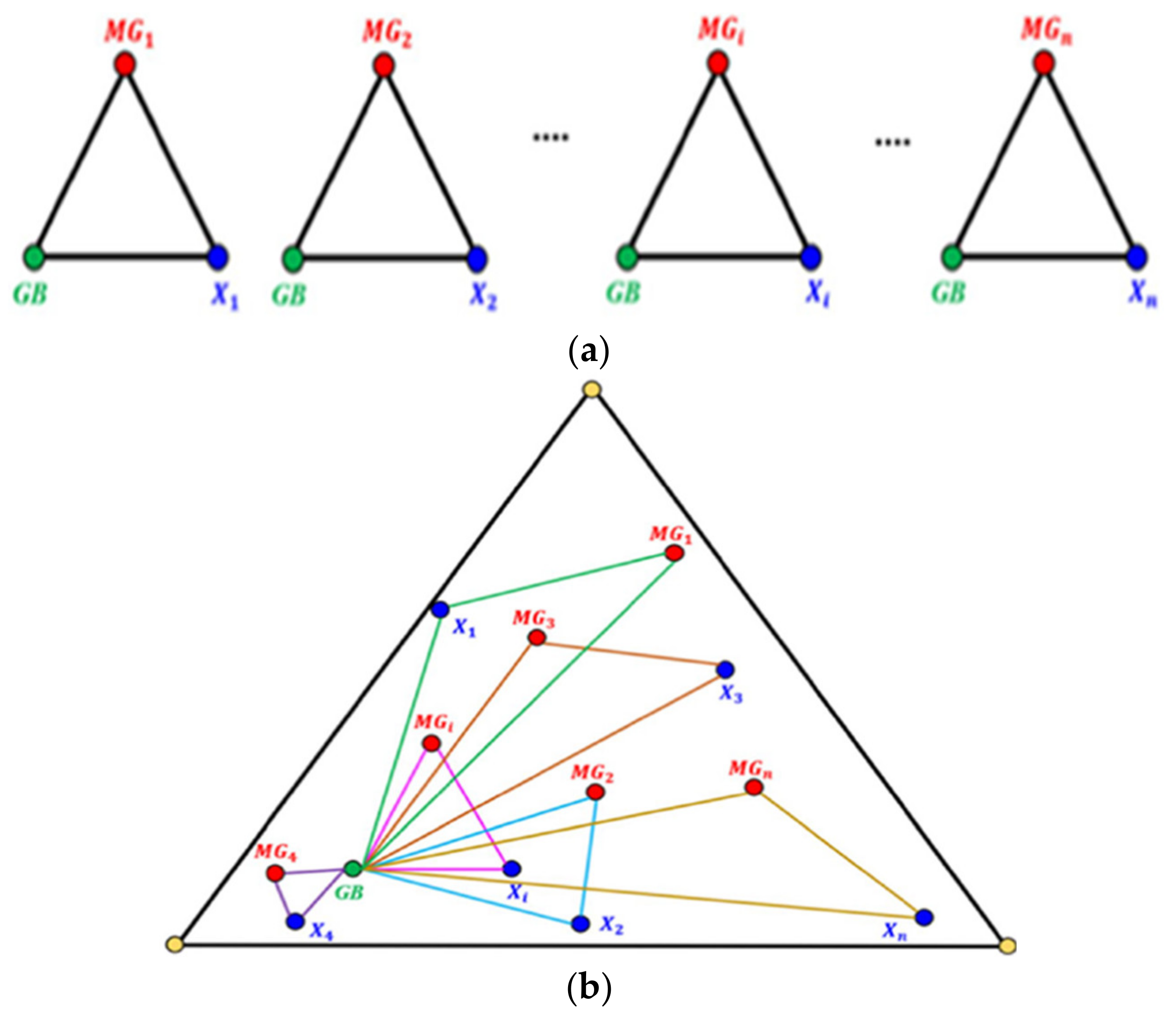
4.2. Mathematical Model

A number of solution candidates ($X$) representing the seeds is assumed by the CGO algorithm. Each candidate solution ($X_i$) consists of some tuneable variables ($X_{i,j}$) representing the seed’s location. The triangle of Sierpinski is considered the exploration field looking for solutions. The following is the mathematical representation:

$$X=\left[\begin{array}{c}{X}_1\\ X_2\\ ⋮\\ X_i\\ ⋮\\ X_n\end{array}\right]=\left[\begin{array}{cccccc}{x}_1^1& x_1^2& \cdots & x_1^j& \cdots & x_1^d\\ x_2^1& x_2^2& \cdots & x_2^j& \cdots & x_2^d\\ ⋮& ⋮& ⋮& ⋮& \ddots & ⋮\\ x_i^1& x_i^2& \cdots & x_i^j& \cdots & x_2^d\\ ⋮& ⋮& ⋮& ⋮& \ddots & ⋮\\ x_n^1& x_n^2& \cdots & x_n^j& \cdots & x_n^d\end{array}\right], \left\{\begin{array}{c}i=1, 2, \dots , n.\\ i=1, 2, \dots , d.\end{array}\right.$$

(13)

where $n$ represents the population size of the exploration field while $d$ refers to the problem dimension. The initialization of the seeds is random as follows:

$$x_i^j\left(0\right)=x_{i,min}^j+rand.\left(x_{i,max}^j-x_{i,min}^j\right), \left\{\begin{array}{c}i=1, 2, \dots , n.\\ i=1, 2, \dots , d.\end{array}\right.$$

(14)

where $x_i^j\left(0\right)$ is the initial population, $x_{i,min}^j$ and $x_{i,max}^j$ refer to the min. and max. values for the $j\mathrm{th}$ design variable, and $rand$ is a random number between 0 and 1.

To finalize the structure of a triangle, the mathematical model generates different seeds within their upper and lower limits. A temporary triangle with three seeds is drawn as follows:

• The Global Best (GB) found so far;
• The Mean Group (MGi) which is the mean values of random seeds;
• The $i\mathrm{th}$ solution candidate ($X_i$).

The vertices of the triangle are GB, MGi and $X_i$. A temporary triangle is generated for each initial seed to generate new seeds to complete a new triangle. The basic schemes of the formation of temporary triangles are shown in Figure 2.

The $i\mathrm{th}$ iteration contains the three corners of a Sierpinski triangle and the seeds obtained in the previous iteration. For new seeds, the temporary triangle is used. The dice are rolled. The seed in $X_i$ is transferred to the GB or to the MGi depending on the resulting color. This is modeled by a random integer function. It generates two integers, either 0 or 1, to allow green or red faces to be selected. According to the chaos game, seed movement should be minimal.

Some generated factorials are used in this regard. The defined process for the first seed is presented mathematically as follows:

$$See{d}_i^1=X_i+{\alpha }_i\times \left({\beta }_i\times GB-{\gamma }_i\times M{G}_i\right), i=1, 2, \dots , n.$$

(15)

where $X_i$ refers to the $ith$ candidate, ${\alpha }_i$ defines the random factorial which limits the seeds’ movement, and ${\beta }_i$ and ${\gamma }_i$ are random integers of 0 or 1 representing the probability of rolling some dice.

Dice of three blue and red faces are used for the second seed (GB). The dice are rolled, and the GB is shifted to $X_i$ or MGi, according to the resulting color. The seed moves towards the $X_i$ when a blue face is raised; if the red face is raised, the seed moves towards the MGi. The second seed goes towards a point on the connecting lines between $X_i$ and MGi. The following equation describes this mathematically:

$$See{d}_i^2=GB+{\alpha }_i\times \left({\beta }_i\times X_i-{\gamma }_i\times M{G}_i\right), i=1, 2, \dots , n.$$

(16)

Regarding the third seed, the dice are rolled. According to the resulting color, the seed moves towards the $X_i$ or GB, which produces only two integrals as 0 and 1. According to some random factors, the seed will travel towards the connected lines between the $X_i$ and GB as expressed in Equation (12).

$$See{d}_i^3=M{G}_i+{\alpha }_i\times \left({\beta }_i\times X_i-{\gamma }_i\times GB\right), i=1, 2, \dots , n.$$

(17)

Another method is also used to create the fourth seed to introduce a mutation step in the location updates of the seeds. The location modification is based on certain changes in the selected decisions. The mathematical model of the process mentioned is:

$$See{d}_i^4=X_i\left(x_i^k=x_i^k+R\right), k=\left[1, 2, \dots , d\right].$$

(18)

where $k$ represents a random integer between 1 and $d$, and $R$ represents random number ranges from 0 to 1.

Four different formulations for ${\alpha }_i$ which regulate the motion limitations of the grain are presented to monitor and change the exploration and exploitation rate of the CGO algorithm as follows:

$${\alpha }_i=\left(x_i^k=x_i^k+R\right)\left\{\begin{array}{c}Rand\\ 2\times Rand\\ \left(\delta \times Rand\right)+1\\ \left(\epsilon \times Rand\right)+\left(~\epsilon \right)\end{array}\right.$$

(19)

where $Rand$ denotes random number ranges from 0 to 1, and $\delta$ and $\epsilon$ refer to random factors between 0 and 1.

The fitness of new candidates is compared with the present ones and those of high fitness are kept, meanwhile, the candidates with lower fitness are rejected.

The pseudo-code of the CGO is expressed as follows:

Generate random initial population ($x_i^j$) of seeds ($X_i$)

Calculate fitness for each seed

Calculate GB

While (t < max. number of iterations)

for i = 1: number of initial seeds

Find $M{G}_i$

Create temporary triangles with$X_i$, GB, and $M{G}_i$

Determine ${\alpha }_i$, ${\beta }_i$, and ${\gamma }_i$

Determine new candidates using Equations (9)–(10).

if new candidates exceed the limits

Modify the candidates and amend them

end if

Calculate the fitness for the new seeds

if new candidates have better fitness than the initial ones

Substitute the worst initial eligible seeds by the new seeds

end if

Update GB if a better fitness is obtained

end for

t = t + 1

end while

return GB

5. Simulation Results

Three test cases of PEMFCs are investigated in this work. The considered PEMFCs are Ballard Mark V, AVISTA SR-12 500 W, and the 6 kW Nedstack PS6 PEMFCs. Experimental measurements are observed for the currents, voltages, and their characteristics. These data are used in the assessment of the efficacy of newly developed CGO by calculating the unknown seven PEM fuel cell design variables. The details of the upper and lower limits of the design variables for the PEMFCs are found in [23,27,28,29]. Since the design variables can be calculated offline, the time needed for simulation is not the highest priority. However, the simulation time of the proposed CGO is also contrasted with the times of other approaches. These simulations are tested on a Microsoft Windows 10 Pro 64-bit version: ‘R2014b’ MATLAB platform (10.0, Build 18363). The MATLAB m-files are run on a Toshiba 2.00 GHz AMD A8-6410 CPU, fitted with 4 GB of RAM. In the following sections, the results of more detailed simulation are shown with respect to the SSE convergence and the I/V polarization curves for the three studied cases of PEMFCs.

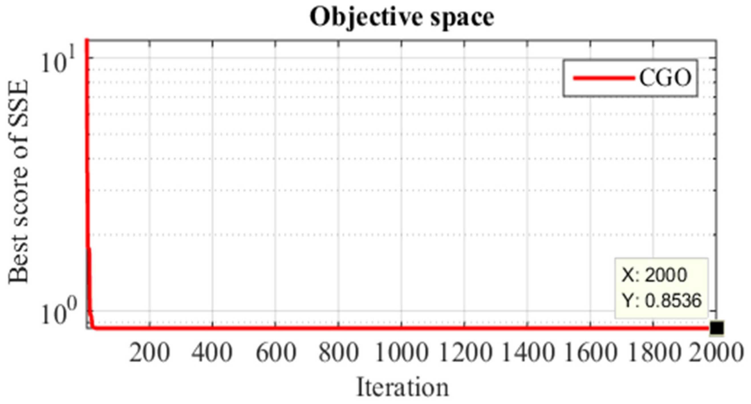
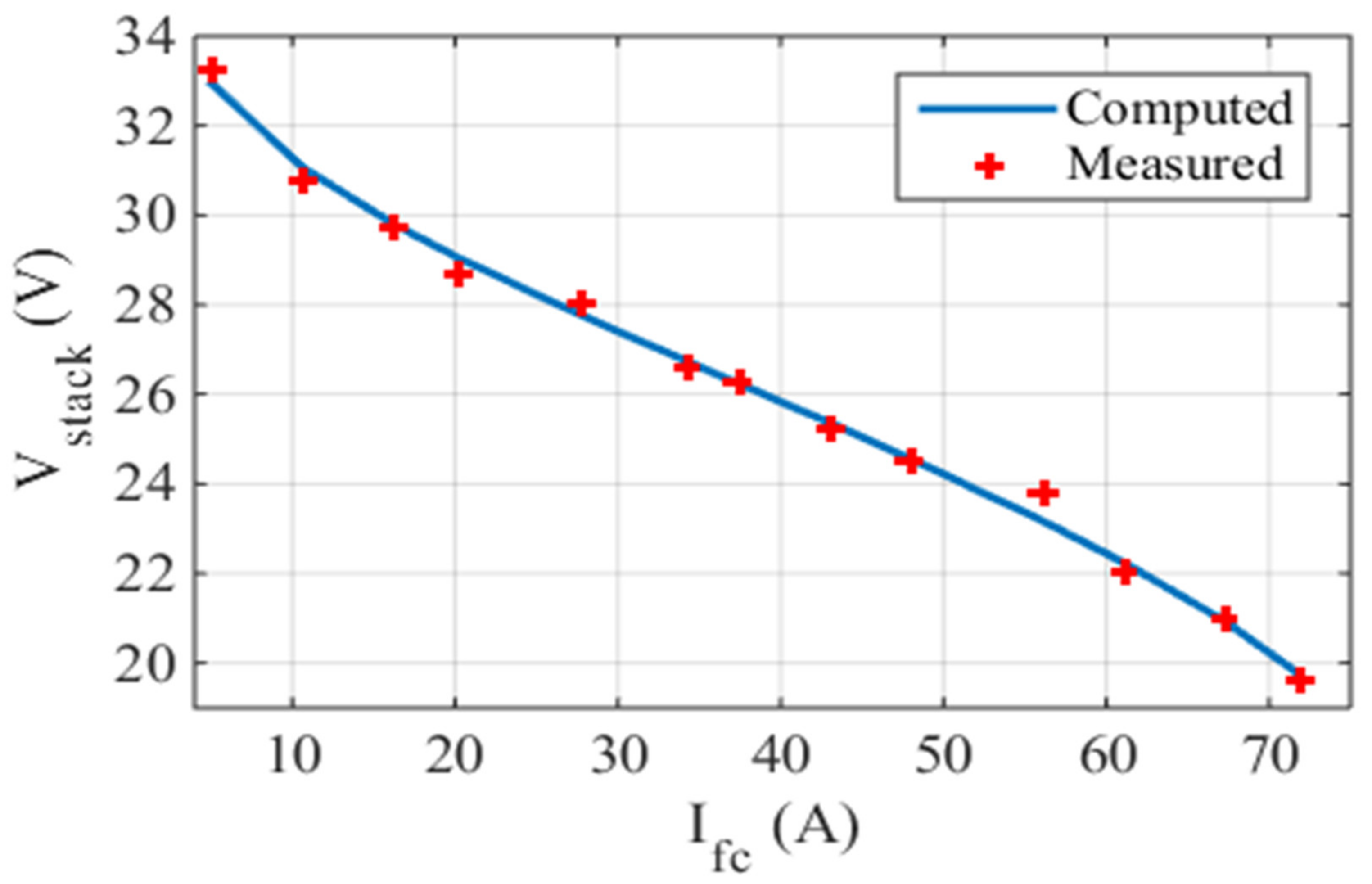
5.1. Case One: The Ballard Mark V

The characteristics of the PEMFC used in this case are illustrated in

Table 1. Characteristics of PEMFC of case one.

Item	Value
No. of series cells	35
Membrane thickness	178 μm
$\mathrm{Surface} \mathrm{area} (M_A)$	50.6 cm2
Thermal limit of the current	70 A
Maximum current density	1.5 A/cm2

. The first case fuel cell used in this experiment contains 35 cells connected in series. The current flowing through the fuel cell under test should not exceed 70 A due to thermal considerations.

Figure 3 depicts the convergence behavior of the objective function during 2000 iterations. The convergence curve represents how the objective function—which is the sum of the squared errors—decreases through the iterations. It can be noted that the proposed CGO algorithm converges fast and smooth. It requires less than 200 iterations to reach a solution close to the final solution at the end of 2000 iterations. For further analysis of the simulation findings of the newly developed optimization method, the I/V curves are provided in Figure 4. It shows a comparison between the estimated voltage by the model and 13 samples of voltages observed experimentally. The blue curve, which is the calculated voltage by the proposed PEMFC model, best fits the 13 voltage readings, which are shown as red crosses, measured experimentally in the lab. The current vs voltage curves show that as the voltage of the fuel cell decreases upon the increase in the drawn current, the appropriate fitting between the estimated and observed voltages is clear. Additionally, the I/P relationship is shown in Figure 5. The blue curve, which is the calculated output power by the proposed PEMFC model, best fits the 13 power readings, which are shown as red crosses, calculated from the measured voltages and currents. As the current increases, more power can be provided by the fuel cell. It validates the exactness of the model and its capability to estimate very close results to those observed in the laboratory.

Further comparisons between the newly developed CGO method versus other optimization methods, used in the literature, are shown in

Table 2. Decision variables for the optimization problem of case one.

Parameter	CGO	HOA	WOA [29]	GHO [23]
${\xi }_1$(V)	−1.192042466678	−0.8532	−1.1978	−0.8532
${\xi }_2\times {10}^{-3}$(V/K)	3.6124342507723	3.3244899099	4.4183	3.4173
${\xi }_3\times {10}^{-5}$(V/K)	4.0797209285374	9.1704275491	9.7214	9.8
${\xi }_4\times {10}^{-5}$(V/K)	−16.283043067932	−15.445073095	−16.273	−15.9555
λ	23	22.999998286	23	22.8458
$R_c$(mΩ)	0.1	0.249053165	0.1002	0.1
β	0.0136000000000001	0.0136	0.0136	0.0136
Population size	50	20	50	60
Number of iterations	2000	2000	2000	2000
Computation time (s)	119.38140	11.4236416	111	95.5
SSE	0.8536075155595	0.9424006399	0.8537	0.871

. It presents the best candidate solutions of the seven design variables (${\xi }_1-{\xi }_4, \mathsf{\lambda }, R_c, \mathrm{and}$β) obtained by each optimization method. This table also shows the settings of the optimization which are: the population size, the number of iterations, and the time taken by each optimization method in seconds to finish the simulation. Finally, the best result of the objective function achieved by each optimization method is shown in the last row.

There are internal losses (voltage drop) in the voltage of the PEMFC such as V_ohmic, V_act, and V_conc. The ohmic losses (V_ohmic) increases linearly upon the current increase. V_act has the highest effect on the total voltage drop (losses). Meanwhile, V_conc has the lowest effect on the total V_losses. The plot of the relation between the internal voltage losses and the current is shown in Figure 6. The simulations are done more than once under different temperatures (30 °C, 50 °C, and 70 °C) at constant partial pressures (${\mathrm{P}}_{{\mathrm{H}}_2}$/${\mathrm{P}}_{{\mathrm{O}}_2}$ = 1/1 atm) to investigate the effect of tuning the temperature on the voltage. This investigation and results are shown in Figure 7. It is noted that the PEMFC output voltage increases when the temperature rises at the same pressure. The difference between the output voltage values at different temperatures increases slightly at higher values of current. In Figure 8, the output power of the fuel cell is plotted against the current. It is observed that the effect of changing the temperature on the output power increases more at higher values of current. Meanwhile, at lower values of current the effect of temperature can hardly be observed.

Besides studying the impact of temperature, the simulations are also done under the different pressures at constant temperature to measure the effect of tuning the pressure on the PEMFC voltage. The resulted I/V curves are shown in Figure 9 which show that the voltage increases when the pressure increases. In Figure 10, the output power of the fuel cell is plotted against the current. It is observed that the effect of changing the pressure on the output power increases at higher values of current. However, when comparing the effect of changing the temperature at constant pressure and vice versa, it is observed that the effect of the temperature on the output power is much higher. Therefore, changing the temperature leads to a wide range of output power from the fuel cell.

5.2. Case Two: The AVISTA SR-12 500 W

The test in the second case of this research study is conducted on 48 cells connected in series, AVISTA SR-12 500 W PEMFC. The specifications of the AVISTA SR-12 500 W PEM fuel cell are found in [25,28,30,31,32]. Figure 11 shows the convergence curve of the objective function for 2000 iterations.

Moreover, Figure 12 presents the I–V characteristics in which the voltage measured for 20 samples is compared with the voltage of the developed model. It can be clearly observed that both voltages are close in value. Regarding the fuel cell of case two, the blue curve of the calculated voltages follows the measured voltage—red marks—much better than that in the case one fuel cell. The relationship between the fuel cell current and power are provided in Figure 13. The results shown in these figures assure the robustness of the model. The values of the measured powers, marked in red, almost satisfy the blue curve of the estimated output power of the fuel cell.

Further numerical comparisons between the newly developed CGO method and other methods in extracting the design variables of the same PEMFC type of case two is given in

Table 3. Decision variables for the optimization problem of case two.

Parameter	CGO	WOA [29]	NNO [32]	GHO [23]
${\xi }_1$(V)	−1.1053135621	−0.8902	−1.0596	−1.1997
${\xi }_2\times {10}^{-3}$ (V/K)	3.506655471	3.3088	3.7435	4.2695
${\xi }_3\times {10}^{-5}$(V/K)	6.726482341	9.75455	9.6902	9.8
${\xi }_4\times {10}^{-5}$ (V/K)	−10.634713544	−10.33	−19.302	−10.1371
λ	21.517713112	22.8311	20.8772	23
$R_c$(mΩ)	0.272639115	0.5677	0.1	0.4638
β	0.150008476	0.1464	0.0161	0.1486
Population size	50	NR	NR	NR
Number of iterations	2000	200	NR	NR
Computation time (s)	116.798459	38.3	33	12.5
SSE	0.000142098	0.0111	0.0117	0.0478

. It provides the values of the seven design variables, the best solution, and the simulation time taken by each optimization method.

The internal voltage losses of the PEMFC of case two are plotted against the fuel cell current in Figure 14. In contrast to the case one fuel cell, the effect of V_conc and V_act on the total voltage losses is more observable. V_conc increases nonlinearly at higher values of the fuel cell current. The ohmic losses has the minimum share in the total voltage losses. The simulations are repeated under different values of temperatures (30 °C, 50 °C, and 70 °C) at constant partial pressures ($P_{H_2}$/$P_{O_2}$ = 1.47/0.2 atm). The effects of changing the temperature on the output voltage and the output power are shown in Figure 15 and Figure 16, respectively. It can be noted that the output voltage of the fuel cell increases upon the temperature rise.

The simulations are further repeated at different pressures under constant temperature. This is done to test the effect of changing the pressure on the voltage. The effects of changing the pressure on the output voltage and the output power are shown in Figure 17 and Figure 18. The voltage increases upon the increase in pressure.

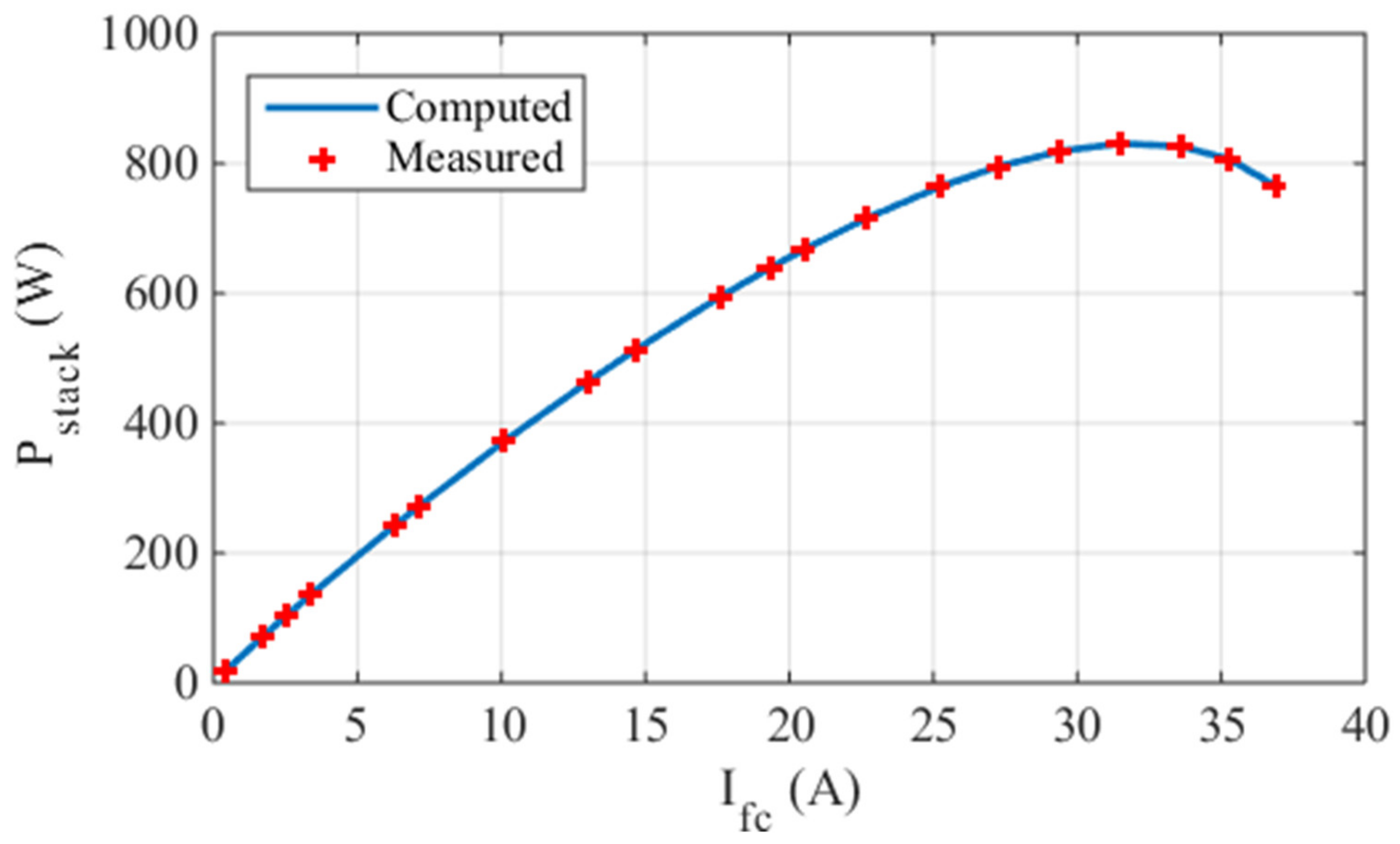
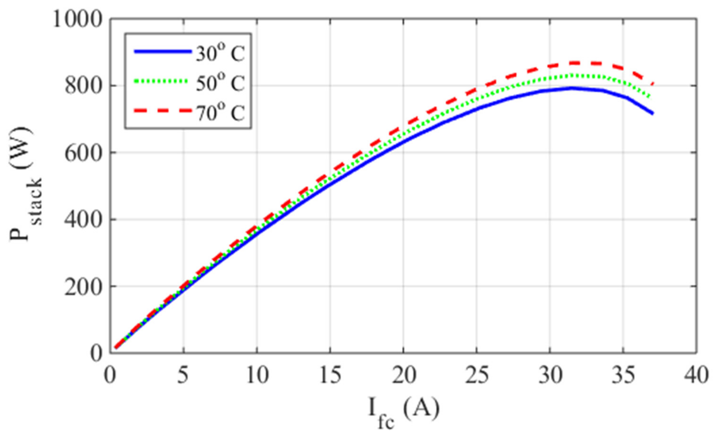
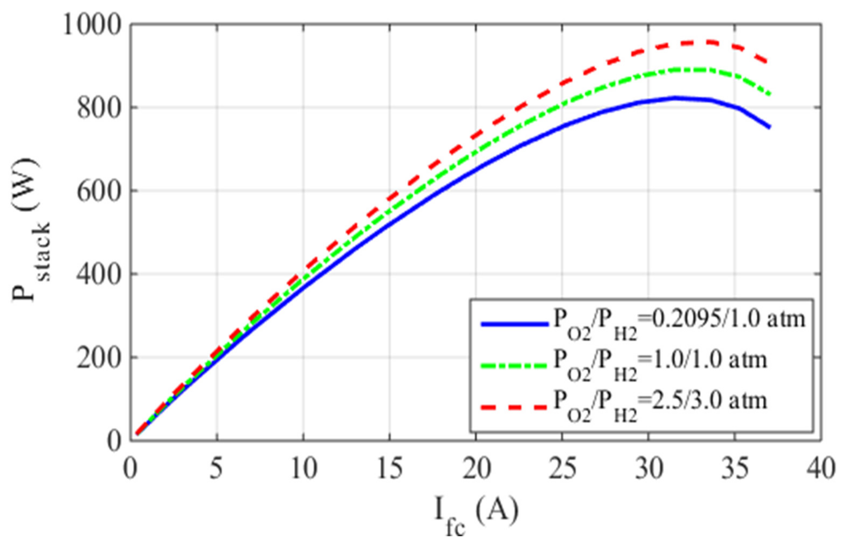
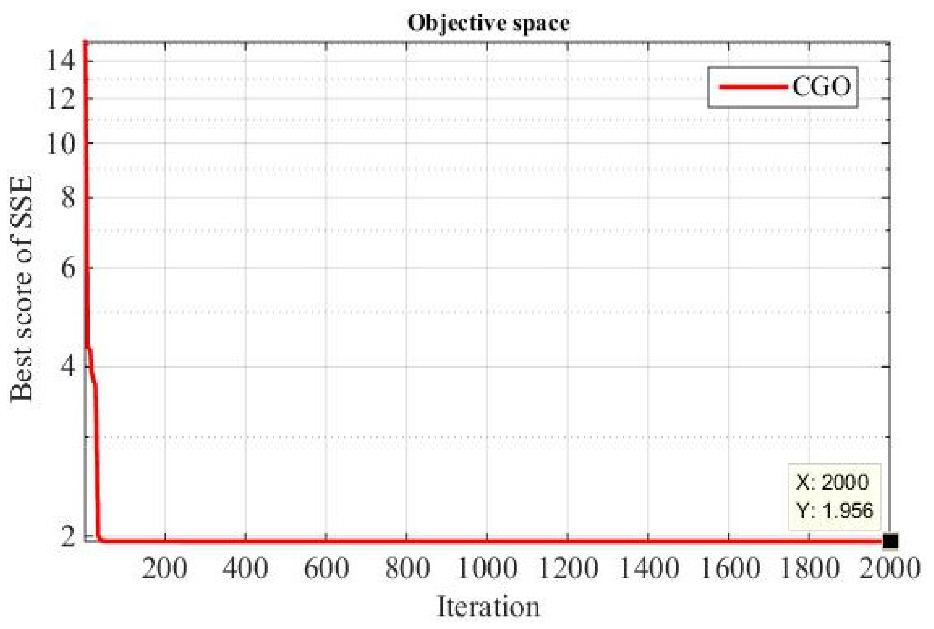
5.3. Case Three: The 6 kW Nedstack PS6

The third considered PEMFC in this study is the 6 kW Nedstack PS6 PEMFC. The specifications of this PEMFC are provided in

Table 4. Characteristics of PEMFC of case three.

Item	Value
No. of series cells	65
Membrane thickness	1.78 mm
$\mathrm{Surface} \mathrm{area} (M_A)$	240 cm2
Max. current density	5 A/cm2

. The test is performed on 65 cells connected in series. The current passing through an area of 1 cm² should not exceed 5 A. The dimensions of the fuel cells under test are shown in the second and third rows in the table.

Similar to the previous two cases, in Figure 19, the change in the values of the FF through the iterations can be seen. For further analysis, the I/V characteristics are provided in Figure 20. It shows a comparison between the estimated voltage and 29 samples of measured voltages. The fitting between the estimated and measured voltages is clear. The relationship between the current and the power is also provided in Figure 21.

Similar to results shown in Table 2 and Table 3 of the first and second fuel cell cases, further comparisons between the newly developed CGO method versus WOA [29] and GHO [23] are presented in

Table 5. Decision variables for the optimization problem of case three.

Parameter	CGO	NNA [32]	SSO [21,25]	GA [23]
${\xi }_1$(V)	−1.14692894516	−0.8535	−0.9719	−1.1997
${\xi }_2\times {10}^{-3}$(V/K)	3.27982148359	2.4316	3.3487	3.4172
${\xi }_3\times {10}^{-5}$(V/K)	3.6043948463	3.7545	7.9111	3.6
${\xi }_4\times {10}^{-5}$(V/K)	−9.54	−9.54	−9.5435	−9.54
λ	13.013946837	13.0802	13	13
$R_c$(mΩ)	0.1	0.1	0.1	0.1376
β	0.0136	0.0136	0.0534	0.0359
Population size	50	NR	NR	NR
Number of iterations	2000	NR	NR	NR
Computation time (s)	91.7770779	NR	NR	NR
SSE	1.955524791	2.14487	2.18067	2.4089

. They present the best candidate solutions of the design variables obtained by each optimization method, the best solution which corresponds to the minimum sum of the square of the errors between the calculated output voltages and the measured output voltages of the fuel cell, and the simulation time taken by each optimization method to finish the simulation and reach such results measured in seconds.

The plot of the internal voltage losses is presented in Figure 22. As seen in this figure, V_act has the maximum effect on the total voltage losses. V_ohmic has the second highest share in the total voltage losses. It increases almost linearly with the fuel cell current. V_conc has a very small value, and it is an almost constant value which is independent of the fuel cell current. The simulations are done more than once under different temperatures (30 °C, 50 °C, and 70 °C) at constant partial pressures (${\mathrm{P}}_{{\mathrm{H}}_2}$/${\mathrm{P}}_{{\mathrm{O}}_2}$ = 1/1 atm). The results of the investigation on the effect of changing the temperature are shown in Figure 23 and Figure 24. The effect is that the voltage increases when the temperature rises. The difference in output voltage increases at higher values of current.

The simulations are also repeated under different pressures at constant temperature to measure the effect of tuning the pressure on the PEMFC voltage. The I/V curves are shown in Figure 25 and Figure 26. From these two figures, it can be seen that the voltage increases when the pressure increases. After observing the results at different temperatures at constant pressure and vice versa, it is concluded that the effect of changing the temperature on the output voltage and the output power is higher than the effect of changing the pressure.

The proposed CGO managed to approximate the optimum values of the design variables of the PEMFCs and the constraints for lowest SSE. The superiority of the CGO PEMFC model reflects the high degree of performance of the CGO and an excellent architecture of the design. Moreover, it has a minimum number of factors and smooth convergence to the optimal solution.

The feasibility of the solution is evaluated by comparing the experimental results with the theoretical simulation results of three PEMFCs. The results achieved by other optimization methods confirmed the privilege of the CGO performance. The implementation of the CGO has resulted in a precise estimation of the PEMFC design variables.

5.4. Robustness Statistical Analysis

Many runs were conducted to further check the robustness of the CGO. The robustness of an optimization algorithm means that many runs should be performed of the same problem to assure that this method can reach such a solution at every run, and that the best solution is not obtained by chance at a single run. For each case, 30 independent runs were performed. The results of case one are shown in detail in

Table 6. Statistical analysis of the proposed CGO algorithm.

Run No.	Case One
1	0.853607516
2	0.853607516
3	0.853607516
4	0.853607516
5	0.853607516
6	0.853607516
7	0.853607516
8	0.853607516
9	0.853607516
10	0.853607516
11	0.853607516
12	0.853607516
13	0.853607516
14	0.853607516
15	0.853607516
16	0.853607516
17	0.853607516
18	0.853607516
19	0.853607516
20	0.853607516
21	1.087297383
22	0.853607516
23	0.853607516
24	0.853607516
25	0.853607516
26	0.853607516
27	0.853607516
28	0.853607516
29	0.853607516
30	0.853607516
Max	1.087297383
Median	0.861397178
Min	0.853607516
Standard Dev.	0.042665737
Variance	0.001820365

.

The values of the standard deviation and the variance are low. This means that the results achieved by each run are very close to each other, indicating the robustness of the proposed optimization process.

6. Conclusions

This article proposed a novel attempt by the CGO to extract the design variables of the PEM fuel cell model. The goal is to achieve an effective PEMFC model that provides comprehensive simulation results for FCs. The FF is formulated to minimize the squaring error between the FC measured voltage and the calculated value. The CGO was introduced to minimize the FF under the problem constraints. The accuracy of the PEMFC model is proved under various temperature and pressure conditions. The efficiency of the constructed model is assessed by comparing the numerical model performance with the experimental results of the three commercial PEMFCs stacks tested. For all case studies, the simulation results coincided with the experimental outcomes. In comparison, the CGO results provided better results than the results based on alternative optimization approaches. This results in a high dominance in the literature of the CGO-based model over other models based on other optimization methods. The proposed CGO algorithm shall be used to solve several other engineering problems such as operation and control of microgrids and smart grids. In future work, the dynamic model of the PEMFCs can be considered instead of the static model. The aging factor of the fuel cell can be also considered.

References

1. Shen, J.; Zhengkai, T.; Siew, H.C. Evaluation criterion of different flow field patterns in a proton exchange membrane fuel cell. Energy Convers. Manag. 2020, 213, 112841. [Google Scholar] [CrossRef]
2. Hussien, A.M.; Mekhamer, S.F.; Hasanien, H.M. Cuttlefish Optimization Algorithm based Optimal PI Controller for Performance Enhancement of an Autonomous Operation of a DG System. In Proceedings of the 2020 2nd International Conference on Smart Power & Internet Energy Systems (SPIES), Bangkok, Thailand, 15–18 September 2020. [Google Scholar]
3. Seleem, S.I.; Hasanien, H.M.; El-Fergany, A.A. El-Fergany. Equilibrium optimizer for parameter extraction of a fuel cell dynamic model. Renew. Energy 2021, 169, 117–128. [Google Scholar] [CrossRef]
4. Sohani, A.; Naderi, S.; Torabi, F.; Sayyaadi, H.; Akhlaghi, Y.G.; Zhao, X.; Talukdar, K.; Said, Z. Application based multi-objective performance optimization of a proton exchange membrane fuel cell. J. Clean. Prod. 2020, 252, 119567. [Google Scholar] [CrossRef]
5. Chen, H.; Liu, B.; Liu, R.; Weng, Q.; Zhang, T.; Pei, P. Optimal interval of air stoichiometry under different operating parameters and electrical load conditions of proton exchange membrane fuel cell. Energy Convers. Manag. 2020, 205, 112398. [Google Scholar] [CrossRef]
6. Agwa, A.M.; El-Fergany, A.A.; Sarhan, G.M. Steady-state modeling of fuel cells based on atom search optimizer. Energies 2019, 12, 1884. [Google Scholar] [CrossRef] [Green Version]
7. Kandidayeni, M.; Macias, A.; Khalatbarisoltani, A.; Boulon, L.; Kelouwani, S. Benchmark of proton exchange membrane fuel cell parameters extraction with metaheuristic optimization algorithms. Energy 2019, 183, 912–925. [Google Scholar] [CrossRef]
8. El-Hay, E.A.; El-Hameed, M.A.; El-Fergany, A.A. El-Fergany. Improved performance of PEM fuel cells stack feeding switched reluctance motor using multi-objective dragonfly optimizer. Neural Comput. Appl. 2019, 31, 6909–6924. [Google Scholar] [CrossRef]
9. Derbeli, M.; Barambones, O.; Farhat, M.; Ramos-Hernanz, J.A.; Sbita, L.; Derbeli, M.; Barambones, O.; Farhat, M.; Ramos-Hernanz, J.A.; Sbita, L. Robust high order sliding mode control for performance improvement of PEM fuel cell power systems. Int. J. Hydrog. Energy 2020, 45, 29222–29234. [Google Scholar] [CrossRef]
10. Karanfil, G. Importance and applications of DOE/optimization methods in PEM fuel cells: A review. Int. J. Energy Res. 2020, 44, 4–25. [Google Scholar] [CrossRef]
11. Gong, X.; Dong, F.; Mohamed, M.A.; Abdalla, O.M.; Ali, Z.M. A secured energy management architecture for smart hybrid microgrids considering PEM-fuel cell and electric vehicles. IEEE Access 2020, 8, 47807–47823. [Google Scholar] [CrossRef]
12. Fathy, A.; Elaziz, M.A.; Alharbi, A.G. A novel approach based on hybrid vortex search algorithm and differential evolution for identifying the optimal parameters of PEM fuel cell. Renew. Energy 2020, 146, 1833–1845. [Google Scholar] [CrossRef]
13. Pan, M.; Li, C.; Liao, J.; Lei, H.; Pan, C.; Meng, X.; Huang, H. Design and modeling of PEM fuel cell based on different flow fields. Energy 2020, 207, 118331. [Google Scholar] [CrossRef]
14. Chugh, S.; Chaudhari, C.; Sonkar, K.; Sharma, A.; Kapur, G.; Ramakumar, S. Experimental and modelling studies of low temperature PEMFC performance. Int. J. Hydrog. Energy 2020, 45, 8866–8874. [Google Scholar] [CrossRef]
15. Taleb, M.A.; Béthouxb, O.B.; Godoy, E. Identification of a PEMFC fractional order model. Int. J. Hydrog. Energy 2017, 42, 1499–1509. [Google Scholar] [CrossRef]
16. Lyu, Z.; Meng, H.; Zhu, J.; Han, M.; Sun, Z.; Xue, H.; Zhao, Y.; Zhang, F. Comparison of off-gas utilization modes for solid oxide fuel cell stacks based on a semi-empirical parametric model. Appl. Energy 2020, 270, 115220. [Google Scholar] [CrossRef]
17. Geem, Z.W.; Noh, J.S. Parameter estimation for a proton exchange membrane fuel cell model using GRG technique. Fuel Cell 2016, 16, 640–645. [Google Scholar] [CrossRef]
18. Chavan, S.; Talange, D.B. Talange. Modeling and performance evaluation of PEM fuel cell by controlling its input parameters. Energy 2017, 138, 437–445. [Google Scholar] [CrossRef]
19. Rao, Y.; Shao, Z.; Ahangarnejad, A.H.; Gholamalizadeh, E.; Sobhani, B. Shark Smell Optimizer applied to identify the optimal parameters of the proton exchange membrane fuel cell model. Energy Convers. Manag. 2019, 182, 1–8. [Google Scholar] [CrossRef]
20. Priya, K.; Sathishkumar, K.; Rajasekar, N. A comprehensive review on parameter estimation techniques for Proton Exchange Membrane fuel cell modelling. Renew. Sustain. Energy Rev. 2018, 93, 121–144. [Google Scholar] [CrossRef]
21. Talatahari, S.; Azizi, M. Optimization of constrained mathematical and engineering design problems using chaos game optimization. Comput. Ind. Eng. 2020, 145, 106560. [Google Scholar] [CrossRef]
22. Mann, R.F.; Amphlett, J.C.; Hooper, M.A.I.; Jensen, H.M.; Peppley, B.A.; Roberge, P.R. Development and application of a generalised steady-state electrochemical model for a PEM fuel cell. J. Power Sources 2000, 86, 173–180. [Google Scholar] [CrossRef]
23. El-Fergany, A. Electrical characterisation of proton exchange membrane fuel cells stack using grasshopper optimiser. IET Renew. Power Gener. 2017, 12, 9–17. [Google Scholar] [CrossRef]
24. Saleh, I.M.M.; Ali, R.; Zhang, H. Simplified mathematical model of proton exchange membrane fuel cell based on horizon fuel cell stack. J. Mod. Power Syst. Clean Energy 2016, 4, 668–679. [Google Scholar] [CrossRef] [Green Version]
25. El-Fergany, A.A. Extracting optimal parameters of PEM fuel cells using salp swarm optimizer. Renew. Energy 2018, 119, 641–648. [Google Scholar] [CrossRef]
26. Talatahari, S.; Azar, B.F.; Sheikholeslami, R.; Gandomi, A. Imperialist competitive algorithm combined with chaos for global optimization. Commun. Nonlinear Sci. Numer. Simul. 2012, 17, 1312–1319. [Google Scholar] [CrossRef]
27. Shaheen, M.A.; Hasanien, H.M.; Alkuhayli, A. A novel hybrid GWO-PSO optimization technique for optimal reactive power dispatch problem solution. Ain Shams Eng. J. 2021, 12, 621–630. [Google Scholar] [CrossRef]
28. Shaheen, M.; Mekhamer, S.F.; Hasanien, H.M.; Talaat, H.E.A. Optimal Power Flow of Power Systems Using Hybrid Firefly and Particle Swarm Optimization Technique. In Proceedings of the 2019 21st International Middle East Power Systems Conference (MEPCON), Cairo, Egypt, 17–19 December 2019; pp. 232–237. [Google Scholar]
29. El-Fergany, A.A.; Hasanien, H.M.; Agwa, A.M. Semi-empirical PEM fuel cells model using whale optimization algorithm. Energy Convers. Manag. 2019, 201, 112197. [Google Scholar] [CrossRef]
30. Zhang, G.; Jiao, K. Three-dimensional multi-phase simulation of PEMFC at high current density utilizing Eulerian-Eulerian model and two-fluid model. Energy Convers. Manag. 2018, 176, 409–421. [Google Scholar] [CrossRef]
31. Qais, M.H.; Hasanien, H.M.; Alghuwainem, S. Transient search optimization: A new meta-heuristic optimization algorithm. Appl. Intell. 2020, 50, 3926–3941. [Google Scholar] [CrossRef]
32. Fawzi, M.; El-Fergany, A.A.; Hasanien, H.M. Hasanien. Effective methodology based on neural network optimizer for extracting model parameters of PEM fuel cells. Int. J. Energy Res. 2019, 43, 8136–8147. [Google Scholar] [CrossRef]
Figure 1. The approach of chaos game to create the Sierpinski triangle.
Sustainability 13 07911 g001
Figure 2. (a) Formation of sub-triangles; (b) sub-triangles inside the exploration field.
Sustainability 13 07911 g002
Figure 3. Convergence curve of the CGO method in the case of Ballard Mark V.
Sustainability 13 07911 g003
Figure 4. Comparison between estimated and practical current–voltage relationship of Ballard Mark V.
Sustainability 13 07911 g004
Figure 5. Comparison between estimated and practical current–power relationship of Ballard Mark V.
Sustainability 13 07911 g005
Figure 6. Internal voltage losses in case of Ballard Mark V.
Sustainability 13 07911 g006
Figure 7. Comparison between I/V curves under various temperatures in case of Ballard Mark V PEMFC.
Sustainability 13 07911 g007
Figure 8. Comparison between I/P curves under various temperatures in case of Ballard Mark V PEMFC.
Sustainability 13 07911 g008
Figure 9. Comparison between I/V curves under various pressures in case of Ballard Mark V PEMFC.
Sustainability 13 07911 g009
Figure 10. Comparison between I/P curves under various pressures in case of Ballard Mark V PEMFC.
Sustainability 13 07911 g010
Figure 11. Convergence curve of the CGO method in case of AVISTA SR–12 500 W.
Sustainability 13 07911 g011
Figure 12. Comparison between estimated and practical current–voltage relationship of AVISTA SR-12 500 W.
Sustainability 13 07911 g012
Figure 13. Comparison between estimated and practical current–power relationship of AVISTA SR-12 500 W.
Sustainability 13 07911 g013
Figure 14. Internal voltage losses in case of AVISTA SR-12 500 W.
Sustainability 13 07911 g014
Figure 15. Comparison between I/V curves under various temperatures in case of AVISTA SR-12 500 W PEMFC.
Sustainability 13 07911 g015
Figure 16. Comparison between I/P curves under various temperatures in case of AVISTA SR-12 500 W PEMFC.
Sustainability 13 07911 g016
Figure 17. Comparison between I/V curves under various pressures in case of AVISTA SR-12 500 W PEMFC.
Sustainability 13 07911 g017
Figure 18. Comparison between I/P curves under various pressures in case of AVISTA SR-12 500 W PEMFC.
Sustainability 13 07911 g018
Figure 19. Convergence curve of the CGO method in case of 6 kW Nedstack PS6.
Sustainability 13 07911 g019
Figure 20. Comparison between estimated and practical current–voltage relationship of 6 kW Nedstack PS6.
Sustainability 13 07911 g020
Figure 21. Comparison between estimated and practical current–power relationship of 6 kW Nedstack PS6.
Sustainability 13 07911 g021
Figure 22. Internal voltage losses in case of 6 kW Nedstack PS6.
Sustainability 13 07911 g022
Figure 23. Comparison between I/V curves under various temperatures in case of 6 kW Nedstack PS6 PEMFC.
Sustainability 13 07911 g023
Figure 24. Comparison between I/P curves under various temperatures in case of 6 kW Nedstack PS6 PEMFC.
Sustainability 13 07911 g024
Figure 25. Comparison between I/V curves under various pressures in case of AVISTA SR-12 500 W PEMFC.
Sustainability 13 07911 g025
Figure 26. Comparison between I/P curves under various pressures in case of AVISTA SR-12 500 W PEMFC.
Sustainability 13 07911 g026