A Hydrodynamic-Based Robust Numerical Model for Debris Hazard and Risk Assessment

Abstract

Debris flow simulations are important in practical engineering. In this study, a graphics processing unit (GPU)-based numerical model that couples hydrodynamic and morphological processes was developed to simulate debris flow, transport, and morphological changes. To accurately predict the debris flow sediment transport and sediment scouring processes, a GPU-based parallel computing technique was used to accelerate the calculation. This model was created in the framework of a Godunov-type finite volume scheme and discretized into algebraic equations by the finite volume method. The mass and momentum fluxes were computed using the Harten, Lax, and van Leer Contact (HLLC) approximate Riemann solver, and the friction source terms were calculated using the proposed splitting point-implicit method. These values were evaluated using a novel 2D edge-based MUSCL scheme. The code was programmed using C++ and CUDA, which can run on GPUs to substantially accelerate the computation. After verification, the model was applied to the simulation of the debris flow process of an idealized example. The results of the new scheme better reflect the characteristics of the discontinuity of its movement and the actual law of the evolution of erosion and deposition over time. The research results provide guidance and a reference for the in-depth study of debris flow processes and disaster prevention and mitigation.

1. Introduction

Debris flows have occurred in many provinces and municipalities in China, and they can be disastrous, often destroying nearly everything in their path and threatening lives, property, and infrastructure [1,2,3]. It is generally believed that a debris flow is a series of processes between the movement of blocks such as collapse and landslide and sediment-bearing water flow, which is formed by the interaction and development of solid-liquid two-phase materials on mountain slopes or channels.

At present, most debris flow models can be clarified as dynamic models and numerical models. The dynamic model of debris flow can be divided into continuous medium, discrete medium, and mixed medium models from the perspective of describing the composition and movement. Continuous medium models can be divided into single-fluid [4,5] and multifluid models [6,7,8,9,10]. The two-phase model is attractive because it can explicitly reveal the relative motions and interactions between the fluid and solid phases. Accordingly, however, the increase in computing costs and also the demand for extra relationships to close the governing equations constrain its applications. Moreover, it is still unclear if they can perform considerably better than traditional single-phase models in terms of modelling accuracy [11]. Single fluid models are generally applicable to debris flows with a large bulk density or a small velocity difference between two phases [12]. Non-Newtonian models include the Bingham body [13], the Bagnold expansion body [14], and the viscoelastic body [15]. The multifluid model mainly refers to the two-component hydrodynamic equations established by considering the momentum exchange between solid and liquid phases. These models can explicitly reveal the relative motion and interaction between the fluid and the solid phase [16]. For example, in the Coulomb mixed flow model, considering the constitutive relationship of granular matter and the interaction force between two phases [17,18,19], Pitman and Le [20] proposed a two-fluid model considering the effect of liquid buoyancy. The discrete medium model simplifies the debris flow into a system composed of a large number of material particles of a certain size. In recent years, with the development of thermal dynamics theory and turbulence theory, the traditional Boltzmann equation has been extended to the study of turbulence and particle flow [21], which provides a method different from the traditional Navier–Stokes (N-S) equation for the theoretical and numerical study of debris flows. The mixed medium model uses a continuous medium model and a discrete medium model to describe the movement of the liquid and solid parts of debris flows. In practice, debris flows are composed of two phases; only certain special types of debris flows, such as mud flows, can be simplified as a phase flow. Although the multifluid model describes the liquid phase and the solid phase with different equations, the equation describing the motion of solid particles is still a continuum model. Generally, the liquid phase of debris flows is a slurry liquid composed of fine particles and water that is smaller than a certain size, which can be regarded as a continuous medium. The solid phase of large particles above a certain size should be described by a discrete medium model. The liquid phase of debris flows is described by a non-Newtonian continuous medium, and the motion equation adopts the two-dimensional depth-averaged shallow water wave equation.

The numerical calculation model of debris flow is closely related to the research problems. Due to the complexity of the debris flow process, a number of models were developed to simulate the flow behavior. The first numerical calculations of debris flows were performed using a one-dimensional homogeneous single-phase continuum model [22,23,24]. With the development of computational fluid dynamics, numerical calculation methods, computer technology, and debris flow theory, numerical approaches have been gradually extended to include multidimensional, heterogeneous, and multiphase models [25,26,27,28,29,30,31,32,33].

It is well known that numerical simulations are an important tool for studying debris flow disaster process. Although full three-dimensional models [34] can increase the precision of high-resolution simulations and may help very detailed resolution of the phenomena, when calculating large practical cases, this method is impractical due to the high calculation cost. In contrast, using the principles of the conservation of mass and momentum, depth-averaged models provide a reasonable balance of completeness and theoretical application and have therefore been broadly applied.

Future science and engineering breakthroughs depend on computing. In recent years, through the implementation of parallelization techniques, there has been a reliable way to significantly reduce computational effort, such as multiprocessing (open MP) and message passing interface (MPI), which allow simulations to be run on cluster machines [35]. Graphics processing units (GPUs) are a new computation engine for high-resolution modeling as computation burdens become increasingly heavy. To resolve the challenge of further accelerating up computations, modern high-performance computer systems increasingly employ GPUs and other accelerators, such as open MP and MPI. Their disadvantages are related hardware cost and energy processor requirements, which usually create a limitation on their practical usage. On the contrary, hardware accelerators, such as GPU, have become a low-cost option, because they can be used on simple personal computers. Previous studies have developed strategies for implementing the pure shallow water equations on graphics processors [36,37]. However, less research has focused on high-resolution terrain using GPU acceleration technology. GPU computing is expected to become more common in future systems. Therefore, programs must be adapted to the use of graphics processors, because graphics processors provide high performance with low costs and power requirements, and therefore they have become the main computing resources of many of the largest supercomputers. Under the framework of a shallow sediment-geomorphology dynamic model, this study focused on a two-dimensional depth-averaged quasi-multiphase mixing model with non-uniform sediment transport to simulate the evolution of debris flows on inclined bed slopes. Namely, by using the GPU Accelerated Surface Water Flow and Transport Model (GAST) model, which can accurately predict debris sediment transport and the debris sediment scouring process, GPU techniques were applied in a numerical model, making it possible to simulate the sediment transport and bed evolution in a high-resolution but efficient way. This method resolves the realistic features of debris sediment transport and uses a GPU-based parallel computing technique to accelerate calculations. The proposed model was validated against experimental benchmark tests. Finally, brief conclusions are drawn.

2. Model Description

Debris flows consist of a multiphase body including solid particles, water, and gas. However, the solid and liquid parts are fully mixed in motion, showing holistic motion. Therefore, debris flows can be regarded as a single fluid that follows the N-S equation of fluid motion. In the process of debris flow movement, the vertical scale is much smaller than the horizontal and vertical scales, so the vertical change in debris flow movement can be ignored. The Saint-Venant equation describing the two-dimensional motion of debris flow can be obtained by the vertical integration of the N-S equation. The vector form of the two-dimensional nonlinear shallow water equation is as follows [38]:

$$\frac{\partial q}{\partial t}+\frac{\partial F}{\partial x}+\frac{\partial G}{\partial y}=S$$

(1)

where,

$$q=\left[\begin{array}{c}\eta \\ q_{{}_x}\\ q_{{}_y}\\ h{c}_s\\ h{\mathrm{c}}_b\\ z_b\end{array}\right]F=\left[\begin{array}{c}{q}_x\\ u{q}_x+\frac{kg{h}^2}{2}\\ u{q}_y\\ q_x{C}_s\\ \beta q_x{C}_b\\ 0\end{array}\right]G=\left[\begin{array}{c}{q}_y\\ v{q}_{{}_y}+\frac{kg{h}^2}{2}\\ v{q}_{{}_y}\\ q_y{C}_s\\ \beta q_y{C}_b\\ 0\end{array}\right]$$

(2)

$$S=\left[\begin{array}{c}0\\ S_{bx}+S_{fx}\\ S_{by}+S_{fy}\\ {\omega }_0\left(C_{sae}-C_{sa}\right)\\ -\frac{\left(q_x{c}_b-\beta q^{*}\right)}{L}\\ \frac{1}{1-p}\left[\alpha \left(\frac{q_x{c}_b-q^{*}}{\beta L}\right)+{\omega }_0\left(1-\alpha \right)\left(C_{sa}-C_{sae}\right)\right]\end{array}\right]$$

(3)

where t is time; x and y are the two-dimensional Cartesian coordinates; $h$ is the flow depth; $F$ and $G$ are the flux vectors of the conserved variables in the x and y directions, respectively; $g$ is the gravitational acceleration with a value of 9.81 m·s⁻²; $u$ and $v$ are the depth-averaged velocities in the and directions, where $q_x=uh$ and $q_y=vh$; hC_s and hC_b are the conserved concentrations of the debris flow suspended load and the bed load, respectively; $z_b$ is the debris flow bed elevation; D and E denote the deposition and entrainment rates, respectively; and the subscripts s and b denote the debris flow suspended load and the bed load, respectively.

$$\begin{gathered} S_{fx}=\frac{{\tau }_{}}{{\gamma }_m}+\frac{\kappa \eta u}{8h{\gamma }_m}+\frac{g{n}^{2}u\sqrt{u^2+v^2}}{h^{1/3}} \\ {S}_{fy}=\frac{\tau }{{\gamma }_m}+\frac{\kappa \eta v}{8h{\gamma }_m}+\frac{g{n}^{2}v\sqrt{u^2+v^2}}{h^{1/3}} \end{gathered}$$

where $\tau$ represents the yield stress, ${\gamma }_m$ represents the unit weight of the debris flow, and $\eta$ represents the viscosity coefficient.

$k$ is the lateral earth pressure coefficient, which depends on the strain rate of the moving material columns [39] and can be expressed as follows:

$$k=\frac{2}{{\cos }^2\phi }\times \left[1\mp \sqrt{1-(1+{\tan }^2\delta )\cos \phi }\right]-1$$

(4)

The conservation Equations (1)–(3) are solved by the GAST model, and the finite volume method in the center format is used to calculate the interface flux. The HLLC approximate Riemann solution of the approximate Godunov method is used. The function of this format is better than that of other formats when dealing with dry elements. This format can better deal with the alternating dry and wet changes in complex terrains and has a strong shock capture ability, considering that the approximate Riemann solution based on HLLC is used to solve the interface flux with only first-order accuracy in space to increase the spatial accuracy of the numerical solution to the second order. At the same time, to avoid the phenomenon of numerical oscillations where the water surface gradient is large after the numerical reconstruction, the model adopts the TVD (Total Variation Diminishing)-MUSCL (Monotonic Upstream-Centered Scheme for Conservation Laws) method for numerical reconstruction. In addition, to ensure that the numerical solution is improved to the second-order accuracy as a whole while maintaining the stability of the numerical solution, the two-order Runge–Kutta format is used for the time step to obtain the second-order accuracy. For dry and wet dynamic boundary treatment, the water depth tolerance is 0.000001 m to distinguish between dry and wet grid cells. The calculation of the friction resistance term uses the split point implicit method to improve stability. In the calculation process, Courant is 0.5, and the CFL (Courant, Friedrichs, Lewy) criterion is used to predict the new time step of the next iteration [40,41,42].

In this work, the proposed numerical scheme was implemented on a GPU using the NVIDIA CUDA toolkit. CUDA (Compute Unified Device Architecture) is a CPU + GPU hybrid programming framework proposed by NVIDIA. The CUAD-based code used a CPU as the Host and the GPU as the co-processor or Device. In the proposed numerical model, the CPU and GPU work together. The CPU is responsible for processing the data transaction and performing serial calculations, whereas the GPU is performing parallel processing tasks. The CUDA parallel computing function running on a GPU is called a kernel function. The C++ programming language is applied on the Host, while the kernel function of the Device must follow the syntax rules and API interface provided by the CUDA. The kernel function can be executed on the GPU after being compiled by the NVCC compiler.

As shown in Figure 1, when performing the parallel computing task, the data are first read into the Host memory through the Host terminal program, and the corresponding GPU device space is allocated for the variable information, such as the grid, initial and boundary conditions, and hydrological and hydraulic parameters. Before calling the kernel function, data must be copied to the device memory. The kernel function is then executed on the GPU for loops. Finally, the computed results are copied back from the Device to the Host for saving and visualization. If the data exchange between the Host and Device memory is too frequent, the data transfer can reduce the performance of the model.

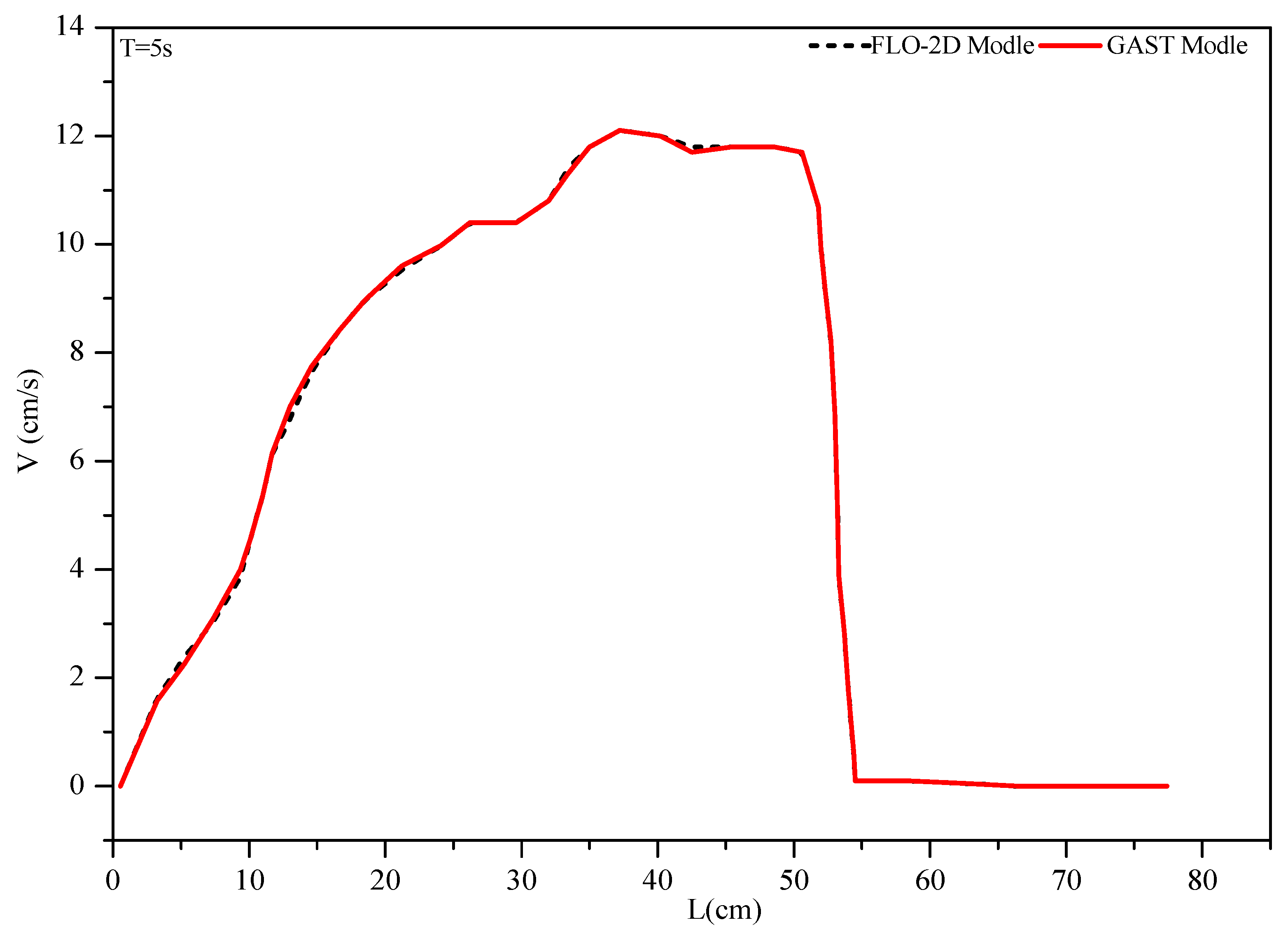
3. Model Verification

To verify the ability of the model to capture the debris flow dynamics on non-corrosive and erosive channel beds, a numerical comparison was carried out using the flume test results of the USGS. In this experiment, two debris flows were considered: debris flows on rough channel beds and debris flows on rough channel bed channel beds covered with erosive sediments. The experimental data for the coarse bed debris flow came from eight repeated USGS flume experiments [43,44]. The experiment recorded unstable and uneven erosive channel bed debris flows from the beginning to the end. The flow front, the flow surface perpendicular to the bed, and the bed deformation were recorded, which basically provides a unique and systematic set of observational data for testing mathematical models of debris flows that can erode channel beds. In all experiments, debris flows were caused by the sudden release of large amounts of water-sediment mixtures. The experimental device, data processing, and material characteristics of the details can be found in [43] and the specific parameters are shown in

Table 1. Simulation parameter attributes.

	${\mathit{\rho }}_{\mathit{s}}$	${\mathit{\rho }}_{\mathit{\omega }}$	$\overline{\mathit{\rho }}$	$\mathit{c}{\mathit{\rho }}_{\mathit{a}}$	${\mathit{\phi }}_1{(}^{\circ })$	${\mathit{\phi }}_2{(}^{\circ })$	$\mathit{\delta }{(}^{\circ })$	${\mathit{\phi }}_{\mathit{v}\mathit{o}\mathit{e}}{(}^{\circ })$	${\mathit{c}}_{\mathit{z}}$	${\mathit{\lambda }}_{\mathit{z}}$
Rough Bare Bed	2700	1000	2020	0	40	40	40	15	12	/
Erodible Bed	2700	1000	2020	0	40	40	40	15	12	0.8
Experimental Value	2700	1000	2010	<400	39	39	40.7	/	/	/

.

Figure 2 and Figure 3 show a comparison between the numerical solutions and the experimental results of the flow height–time curves of rough bare bed and erodible sediments. The experimental curve in Figure 3 corresponds to experiment C by Iverson [45]. Additionally, the results are close to those of the simulation in [38]. The simulation curve of the water flow height with time is basically consistent with the experimental results. For the erodible channel bed, the time to reach two positions is slightly earlier than the experimental results. Therefore, this simple model with a constant pore pressure coefficient can capture complex debonding flow dynamics [45]. The results show that the model established in this paper can be used for debris flow simulations.

4. Numerical Tests

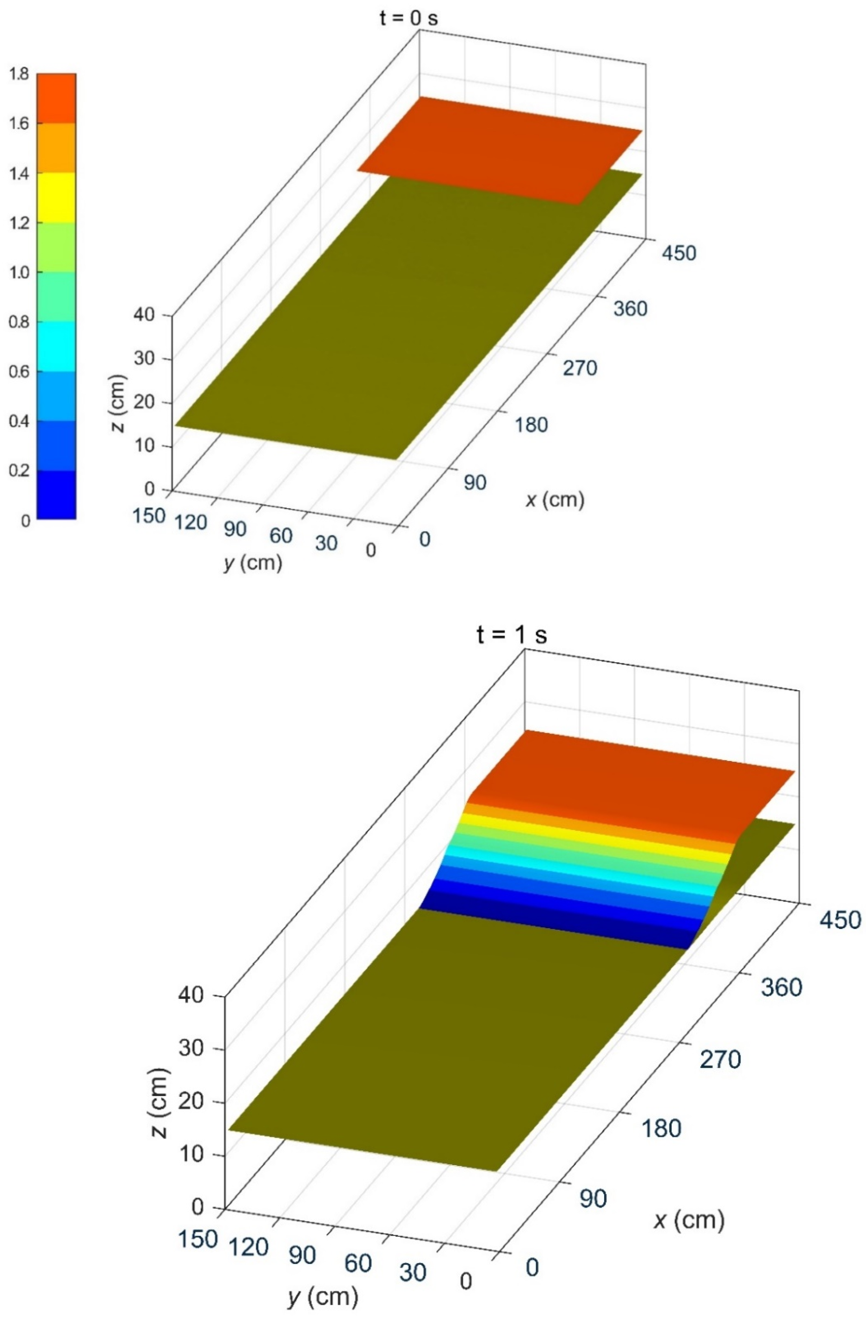
4.1. Numerical Simulation of Dam-Breaking Debris Low

The general process of the dam-breaking debris flow is that the water flow is fully topped, then the dam body is flattened, and finally, the entire body is broken to form a debris flow. To verify the rationality of the proposed GAST model, the experiment performed by Komatina in 1997 [46] was selected as an example. This experiment has been used by many scholars to verify numerical models that simulate dam-break debris flows. The length of the water tank in the calculation example was 4.5 m, and the width was 1.5 m. The fluid was a mixture of water and kaolinite clay with solid particles of different concentrations. The average diameter of the particles was 0.006 mm. The proportion of clay material was 2.65. The dam-breaking debris flow was simulated at different moments in the smooth flume. The measured slurry was placed in a container with a length of 2 m and a width of 1.5 m at the top of the water tank, with an initial height of 1 m, and the slurry was blocked by a movable baffle.

Dam-break flows are caused by a mixture being released by the reservoir located upstream of the flume. The discharge caused by the sudden removal of gates between reservoirs and rivers is actually instantaneous. The propagating positive waves were captured by cameras. The velocity of the wave and the form of the wave array were digitally recorded. In each experimental process, the level was also continuously monitored. The initial reservoir depth was 10–30 cm, the channel bed slope was 0.0–0.1%, and the volume concentration was different. The channel slope was 0.1%. The wavefront propagation time increased significantly as the concentration increased. For different concentrations, the simulated and observed values are basically consistent, and it is clear that the model is reliable (Figure 4).

At the beginning of the test, the movable baffle was pulled out to allow the slurry to flow freely, and the deformation of the mud front edge and the movement distance of the front edge were recorded at each time node. The simulation time was 10 s, five typical moments of t = 0 s, t = 1 s, t = 5 s, t = 7 s, and t = 10 s were selected, and the movement distance of the mud front obtained by numerical simulation changed with time. Figure 5 shows that the destruction process of the dam-breaking debris flow can be divided into three stages: when t = 0 s, the flow was in a static state; when t = 1 s, with the continuous infiltration of water, the shear surface developed and reached the middle of the tank; and when t = 5 s, the debris flow moved quickly and started to move to the bottom of the tank. In addition, the color in the flume was red at first and gradually transitioned to a green and blue distribution, indicating that the material sources in the flume began to erode after a certain period of time, forming a complete debris flow process.

A horizontal distance simulation over time in different stages in the drainage trough is shown in Figure 6. The maximum horizontal distance reached from 0–15 s was 120 cm. At 0 s, the debris flow deposits rapidly accumulated, but the sink was straight and still had a certain capacity for entrainment. As a result, the debris flow curve displays a slight downward trend after rapid sedimentation. At 5 s and 7 s, the horizontal distance of the debris flows first increased rapidly and then increased gradually from 68–105 cm. The initial rapid increase was caused by the rapid sedimentation of the debris flow material.

In Figure 7, a resting velocity of 0 m/s can be observed at t = 0 s. As the sliding speed increased, the velocity accumulation peaked at t = 5 s, with the speed reaching 12 cm/s, and the corresponding horizontal distance was 40 cm. As the debris flow moved in the horizontal direction, the mud depth showed a tendency to fluctuate and thicken—that is, there was a possibility of accumulation—additionally, the area of the debris flow was approximately 330 m². At t = 15 s, the debris flow eroded the channel bed and moved to the end of the flume. The slope of the breach continued to slide, which made the breach wider than it was at t = 7 s. The velocity was mostly between 10 cm/s and 5.5 cm/s, and the maximum velocity was 17.5 cm/s.

In summary, the reasons for this phenomenon may be attributed to the following points. Some researchers think that more comparisons of fixed-bed and entrainment models must be conducted to judge the reliability of the suggested enhancement of the model calibration process [47]. Although the two models used to simulate the propagation are based on different rheological laws, the results obtained in terms of debris flow paths and, more in general, of inundation depth and velocity, are very similar [48]. Bed entrainment plays a major role in determining the whole propagation pattern; however, there can be different aspects of erosion in nature [49]. Because of the addition of material from the ground surface to the moving mass, the reduction in kinetic energy of the system might be greater than the increase in its potential energy. However, those complex behaviors also depend on which erosion mechanism takes place, which flow theologies are involved, and how the mass and momentum productions are considered in the dynamical model equations. This requires further research.

The FLO-2D model is a tool adopted worldwide for the simulation of debris flow phenomena and hydraulic flooding of urban areas [47,48]. At present, the FLO-2D model has possibly been most widely applied to natural debris flows or compared with other models [49,50,51,52]. In order to verify the simulation results of the GAST model, this paper compares the simulation results with those of the FLO-2D model by simulating the sliding phenomenon at different stages. It was found that the simulated horizontal distance and debris flow velocity were basically consistent with the actual physical process. This verifies the rationality of the GAST numerical model in this paper.

To objectively compare the accuracy of the model, common statistical indicators including the root mean square error (RMSE), coefficient of determination (R²), and mean relative error (MRE) were adopted, and the index calculation formula is shown in Equation (5).

An RMSE value of zero indicates a perfect fit Equation (5). If the value is less than half of the standard deviation of the observations, the model performance is considered to be good.

$$RMSE=\sqrt{\frac{{\displaystyle {\sum }_{i=1}^n{(M_i-S_i)}^2}}{N}}$$

(5)

The coefficient of determination R² reflects the degree of coincidence of the simulated and observed final bed and water levels (Equation (6)). The closer R² is to 1, the higher the degree of coincidence with the simulated runoff process is. R² can be calculated as follows:

$$R^2=\frac{{\left|{\sum }_{i=1}^{\mathrm{nd}}\left(M-\overline{M}\right)\left(S-\overline{S}\right)\right|}^2}{{\sum }_{I=1}^{\mathrm{nd}}{\left(M_i-\overline{M}\right)}^2{\sum }_{I=1}^{\mathrm{nd}}{\left(S_i-\overline{S}\right)}^2}$$

(6)

The efficiencies of the simulated and observed processes were evaluated by the coefficient of relative error (MRE), calculated as follows (Equation (7)):

$$MRE=\frac{1}{n}\sum _{i=1}^n\frac{\left|S_i-M_i\right|}{Mi}\times 100\%$$

(7)

where M is an observed value, S is a simulated value, $\overline{M}$ is a mean observed value, $\overline{S}$ is a mean simulated value, and N is the sample number. The calculation results for the three indicators are compared in

Table 2. Performance comparison for different model for the depth and velocity level simulations.

Content	Time	RMSE	R2 (%)	MRE
Depth-L	5 s	0.1822	95.8	1.325
	7 s	0.0208	97.2	1.289
	10 s	0.0459	96.4	1.244
Average		0.2489	96.4	1.286
Velocity-L	5 s	0.035	90.2	1.412
	7 s	0.056	97.6	1.366
	10 s	0.062	94.5	1.402
Average		0.051	94.1	1.393

.

As shown in Table 2 and Figure 6 and Figure 7, the proposed GAST model was reliable and could achieve good predictive results for morphological processes. The comparative analysis showed that the accuracy of the simulated results could also be reflected by R², RMSE, and MRE. Figure 6 and Figure 7 show the correlation between the measured and simulated depth and velocity values based on the corresponding coefficient of determination. Therefore, the predictive model proposed in this paper shows strong generalizability. Meanwhile, the model performance was acceptable.

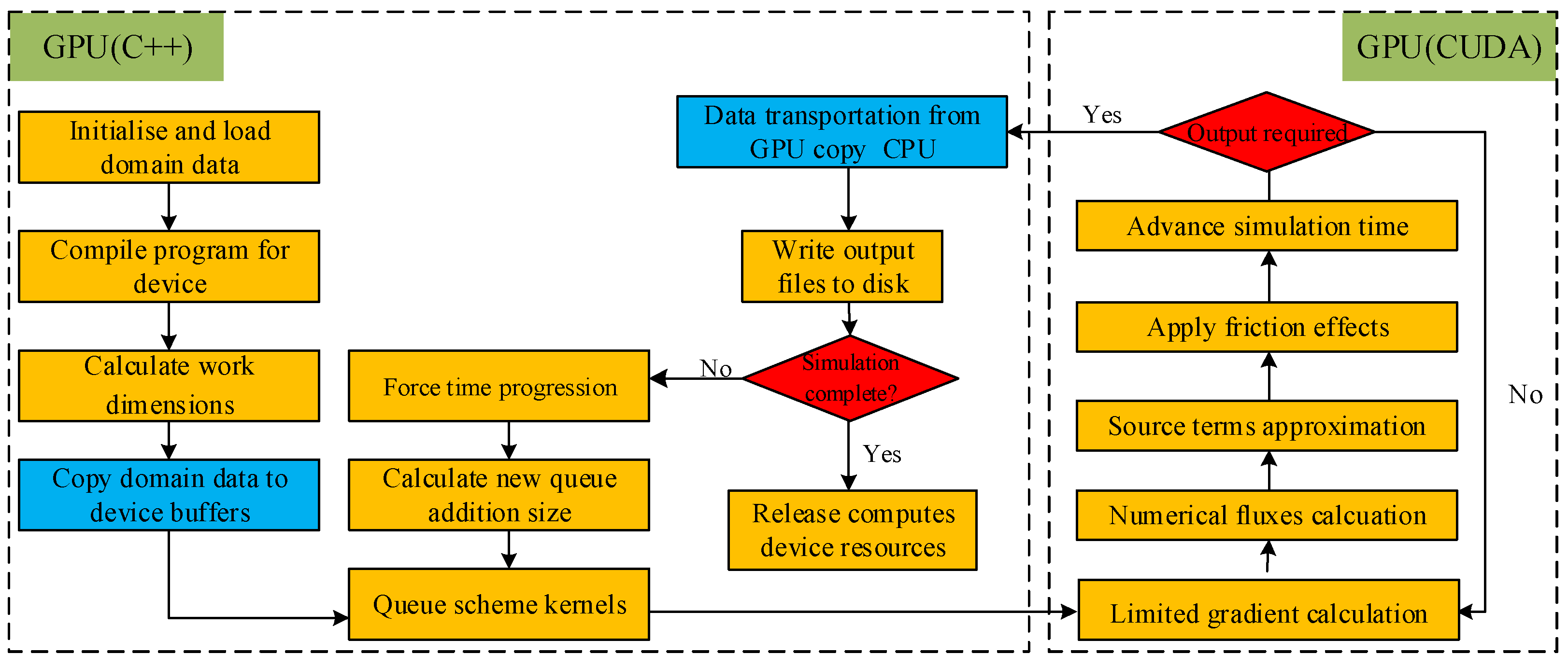
4.2. GPU and CPU Runtime

Several tests were performed to prove the validity of our GAST model. All tests were conducted using the same computational devices; the GPU was an NVIDIA GeForce GTX 1080 Ti with 16 G memory, and the CPU was an Intel (R) Core (TM) i7-6700 K CPU @ 4.00 GHz.

The debris-flow-prone area in Pusa Village, Guizhou Province, China, covers 2.68 km². The 12 m resolution, high-precision terrain was simulated using the GAST model for 3 h. The number of calculation grids for the 12 m resolution terrain was 2,592,280, the CPU calculation time was 5151.9 s, and the GPU time was 352.21 s. The hazard CPU and GPU simulation times and the results of the debris-flow-prone area were compared using the single-core Intel CoreTM i7-7700 as a comparison standard, and the speedup ratio was set to 1. Compared with the Intel CoreTM i7-7700 (single-core CPU), the mudslide simulation calculation performed using the NVIDIA GeForce GTX 1080 (GPU) was up to 14.62 times more efficient. Therefore, the GPU computing power far exceeded the CPU computing power (

Table 3. CPU and GPU simulation performance comparison for the execution time and speed up for a removable debris flow.

CPU (Four Cores)	GPU
t	t	sup
5151.9 s	352.21 s	14.62

).

To compare the computational costs of the current complete GAST model [53,54] and the two-phase model,

Table 4. Relative CPU and GPU runtimes of the GAST model and the two-phase model.

Model	FB (Fixed Bed)	EB (Erodible Bed)
Two-phase model (Li et al. 2017a, b)	1.22	1.31
GAST (GPU Accelerated Surface Water Flow and Transport Model)	0.75 0.80 0.79 1.00	0.98 1.10 1.04 0.97
Speed-up (Four averages)	18–35%	16–25%

shows the CPU run time and GPU time of the two models in the FB and EB cases. The results show that the erosive bed required more processing time than the fixed bed because the former involved the bed evolution equation, which reflects the mass exchange between the flow and the bed.

However, the calculation time of the GAST model was 16–35% faster than that of the two-phase model [53,54]. In addition, if the number of equations increases, the computation time is bound to increase [53,54]. Therefore, it can be predicted that the central processor run time of the two-phase model will inevitably increase compared with that of the GAST model, especially in the simulation of large-scale debris flows.

5. Discussion

Some researchers think that more comparisons of fixed bed and entrainment models must be conducted to judge the reliability of the suggested enhancement of the model calibration process [53]. Although the two models used to simulate the propagation are based on different rheological laws, the results obtained in terms of debris flow paths and, more in general, of inundation depth and velocity, are very similar [54]. Bed entrainment plays a major role in determining the whole propagation pattern; however, there can be different aspects of erosion in nature [55]. Because of the addition of material from the ground surface to the moving mass, the reduction in kinetic energy of the system might be greater than the increase in its potential energy. However, those complex behaviors also depend on which erosion mechanism takes place, which flow theologies are involved, and how the mass and momentum productions are considered in the dynamical model equations. This can probably be the situation for flows in moderate to low slope angles. Nevertheless, the erosion related mobility can be site- and material-specific. This requires further research.

Regarding the effect of density change for debris flow, some research finds that for debris flow in the jump to the fast-moving incoming flow, compared to the predicted runup height, the difference in the predicted impact load appears to be even negligible [56]. Compressibility in natural debris flow is highly variable in its temporal and spatial distribution. Especially for nearly liquefied debris flows for where state of material varies de-pending on the barrier deformation pattern, the active state of downstream-jump debris material due to barrier deflection facilitates to further reduce the impact load. The contribution of jump volume resistance to the load attenuation obviously depends on the jump length, which in turn is controlled by the incoming flow properties. The compressibility (density change) does not significantly contribute to the load attenuation.

At present, because of the complicated solid–fluid interaction within the two-phase debris flow [9,34,47], possible scale-dependent effects [17,18,19] cannot be explicitly considered. Some researchers conclude that the peak flow depth being out of sync with the peak velocity (a tapered flow front) causes of this discrepancy. Characterization of the debris properties is more important than selection of debris impact model. However, parameter values are constrained to differing degrees in different types of flows. Perhaps the greatest limitation on the model’s predictive capability results from the assumption that flows maintain constant masses as they move down slope. Mass change is an important feature of some debris flow sand avalanches, and although mass change terms may be appended to the model equations with little difficulty, the magnitude of such terms depends on external forces, which are poorly constrained in most instances [57].

In the future, the application of the novel erosion rate model to experimental and complex natural events of debris flow and avalanche mixtures would require substantial additional work and corresponding parameter estimates, either derived from field measurements or back calculations, involving observation data, which, therefore, must be deferred to some future contributions [9]. At the same time, debris flow hazard is viewed as a threat that has the potential to overwhelm people, property, and the environment. It is a pre-existing condition that can turn into a catastrophe depending on the influence of exogenous and endogenous factors. We should use multiple models for comprehensive research, such as the Pressure and Release (PAR) Model and Access Model, the Hazards-of-Place (HOP) Model, the Regions of Risk Model [58], and so on. These models techniques can significantly contribute to the deeper understanding of debris flow hazard, risk, and vulnerability, providing better representation and visualization of human–environment interaction [59,60].

6. Conclusions

Based on the theory of shallow water deposition morphology dynamics, a GAST model suitable for debris flow was developed. The model was established under the framework of a Godunov-type finite volume scheme, and the control equation was solved by a completely conservative numerical algorithm. Compared with previous experiments and actual debris flows, the new model can reflect the dynamic process of debris flows. Although there are other two-phase models that perform better than the GAST model, the GAST model is still attractive because GPU acceleration technology greatly improves the computational time of the model. The experimental results in this paper prove that GPU acceleration technology can improve the performance by 14.62 times and increase the computational efficiency by 16–35%, especially in applications that require a large amount of high-performance computing. The general-purpose computing of GPUs will address areas and problems that require considerable manual computing in a low-cost and high-efficiency manner.

References

1. Wang, Y.; Nie, L.; Zhang, M.; Wang, H.; Xu, Y.; Zuo, T. Assessment of Debris Flow Risk Factors Based on Meta-Analysis—Cases Study of Northwest and Southwest China. Sustainability 2020, 12, 6841. [Google Scholar] [CrossRef]
2. Li, Q.; Lu, Y.; Wang, Y.; Xu, P. Debris Flow Risk Assessment Based on a Water–Soil Process Model at the Watershed Scale Under Climate Change: A Case Study in a Debris-Flow-Prone Area of Southwest China. Sustainability 2019, 11, 3199. [Google Scholar] [CrossRef] [Green Version]
3. Lyu, H.-M.; Shen, J.S.; Arulrajah, A. Assessment of Geohazards and Preventative Countermeasures Using AHP Incorporated with GIS in Lanzhou, China. Sustainability 2018, 10, 304. [Google Scholar] [CrossRef] [Green Version]
4. Armanini, A.; Fraccarollo, L.; Larcher, M. Liquid-granular channel flow dynamics. Powder Technol. 2008, 182, 218–227. [Google Scholar] [CrossRef]
5. Rosatti, G.; Begnudelli, L. Two-dimensional simulation of debris flows over mobile bed: Enhancing the TRENT2D model by using a well-balanced Generalized Roe-type solver. Comput. Fluids 2013, 71, 179–195. [Google Scholar] [CrossRef]
6. Pitman, E.B.; Le, L. A two-fluid model for avalanche and debris flows. Philos. Trans. R. Soc. Math. Phys. Eng. Sci. 2005, 363, 1573–1601. [Google Scholar] [CrossRef] [PubMed]
7. Pelanti, M.; Bouchut, F.; Mangeney, A. A Roe-Type scheme for two-phase shallow granular flows over variable topography. ESAIM Math. Model. Numer. Anal. 2008, 42, 851–885. [Google Scholar] [CrossRef] [Green Version]
8. Pailha, M.; Pouliquen, O. A two-phase flow description of the initiation of underwater granular avalanches. J. Fluid Mech. 2009, 633, 115–135. [Google Scholar] [CrossRef]
9. Pudasaini, S.P. A general two-phase debris flow model. J. Geophys. Res. Earth Surf. 2012, 117. [Google Scholar] [CrossRef]
10. Greco, M.; Iervolino, M.; Leopardi, A.; Vacca, A. A two-phase model for fast geomorphic shallow flows. Int. J. Sediment. Res. 2012, 27, 409–425. [Google Scholar] [CrossRef]
11. Xia, C.C.; Li, J.; Cao, Z.X.; Liu, Q.Q.; Hu, K.H. A quasi single-phase model for debris flows and its comparison with a two-phase model. J. Mt. Sci. 2018, 15, 1071–1089. [Google Scholar] [CrossRef]
12. Da-you, L.I.U. Discussion on the Concepts of Two-Phase Flow, Multiphase Flow, Multifluid Model and Non-Newtonian Flow. Adv. Mech. 1994, 24, 66–74. [Google Scholar]
13. Johnson, A.; Rahn, P. Mobilization of debris flows. Z. Fur Geomorphol. 1970, 9, 168–186. [Google Scholar]
14. Takahashi, T. Mechanical characteristics of debris flow. J. Hydraul. Div. 1978, 104, 1153–1169. [Google Scholar] [CrossRef]
15. Chen, C. General solutions for viscoplastic debris flow. J. Hydraul. Eng. 1988, 114, 259–282. [Google Scholar] [CrossRef]
16. Chen, H.X.; Zhang, L.M.; Gao, L.; Yuan, Q.; Lu, T.; Xiang, B.; Zhuang, W.L. Simulation of interactions among multiple debris flows. Landslides 2017, 14, 595–615. [Google Scholar] [CrossRef]
17. Iverson, R.M. The physics of debris flows. Rev. Geophys. 1997, 35, 245–296. [Google Scholar] [CrossRef] [Green Version]
18. Denlinger, R.P.; Iverson, R.M. Flow of variably fluidized granular masses across three-dimensional terrain:2. Numerical predictions and experimental tests. J. Geophys. Res. 2001, 106, 553–566. [Google Scholar] [CrossRef]
19. Bouchut, F.; Fernández-Nieto, E.D.; Mangeney, A.; Narbona-Reina, G. A two-phase shallow debris flow model with energy balance. ESAIM Math. Modell. Numer. Anal. 2015, 49. [Google Scholar] [CrossRef] [Green Version]
20. Beppu, M.; Inoue, R.; Ishikawa, N.; Hasegawa, Y.; Mizuyama, T. Numerical simulation of debris flow model by using modified MPS method with solid and liquid particles. J. Jpn. Soc. Eros. Control Eng. 2011, 63, 32–42. [Google Scholar]
21. Chen, S.; Doolen, G.D. Lattice Boltzmann method for fluid flows. Annu. Rev. Fluid Mech. 2003, 30, 329–364. [Google Scholar] [CrossRef] [Green Version]
22. De Leon, A.A.; Jeppson, R.W. Hydraulics and Numerical Solutions of Steady-State but Spatially Varied Debris Flow; Utah Water Research Laboratory: Logan, UT, USA, 1982; p. 95. [Google Scholar]
23. Schamber, D.R.; MacArthur, R.C. One-dimensional model for mud flows. NASA STI/Recon. Tech. Rep. 1985, 86, 1334–1339. [Google Scholar]
24. Takahashi, T. Estimation of potential debris flows and their hazardous zones: Soft countermeasures for a disaster. Nat. Disaster Sci. 1981, 3, 57–89. [Google Scholar]
25. Iverson, R.M. Elementary theory of bed-sediment entrainment by debris flows and avalanches. J. Geophys. Res. 2012, 117, 406. [Google Scholar] [CrossRef]
26. Han, G.; Wang, D. Numerical modeling of Anhui debris flow. J. Hydraul. Eng. 1996, 122, 262–265. [Google Scholar] [CrossRef]
27. Hungr, O. A model for the runout analysis of rapid flow slides, debris flows, and avalanches. Can. Geotech. J. 1995, 32, 610–623. [Google Scholar] [CrossRef]
28. Iverson, R.M.; Denlinger, R.P. Flow of variably fluidized granular masses across three-dimensional terrain: Coulomb mixture theory. J. Geophys. Res. 2001, 106, 537–552. [Google Scholar] [CrossRef]
29. McDougall, S.; Hungr, O. A model for the analysis of rapid landslide motion across three-dimensional terrain. Can. Geotech. J. 2004, 41, 1084–1097. [Google Scholar] [CrossRef]
30. O’brien, J.; Julien, P.; Fullerton, W. Two-dimensional water flood and mudflow simulation. J. Hydraul. Eng. 1993, 119, 244–261. [Google Scholar] [CrossRef]
31. Hussin, H.Y.; Quan Luna, B.; van Westen, C.J.; Christen, M.; Malet, J.P.; van Asch, T.W.J. Parameterization of a numerical 2-D debris flow model with entrainment: A case study of the Faucon catchment, Southern French Alps. Nat. Hazards Earth Syst. Sci. 2012, 12, 3075–3090. [Google Scholar] [CrossRef]
32. De Haas, T.; Braat, L.; Leuven, J.R.; Lokhorst, I.R.; Kleinhans, M.G. Kleinhans. Effects of debris flow composition on runout, depositional mechanisms, and deposit morphology in laboratory experiments. J. Geophys. Res. Earth Surf. 2015, 120, 1949–1972. [Google Scholar] [CrossRef] [Green Version]
33. Lanzoni, S.; Gregoretti, C.; Stancanelli, L.M. Coarse-grained debris flow dynamics on erodible beds. J. Geophys. Res. Earth Surf. 2017, 122, 592–614. [Google Scholar] [CrossRef]
34. Pudasaini, S.P.; Mergili, M. A multi-phase mass flow model. J. Geophys. Res. Earth Surf. 2019, 124, 2920–2942. [Google Scholar] [CrossRef] [Green Version]
35. Lacasta, A.; García-Navarro, P.; Burguete, J.; Murillo, J. Preprocess static subdomain decomposition in practical cases of 2D unsteady hydraulic simulation. Comput. Fluids 2013, 80, 225–232. [Google Scholar] [CrossRef] [Green Version]
36. Kalyanapu, A.J.; Siddharth, S.; Pardyjak, E.R.; Judi, D.R.; Burian, S.J. Assessment of GPU computational enhancement to a 2D flood model. Environ. Model. Softw. 2011, 26, 1009–1016. [Google Scholar] [CrossRef]
37. Vacondio, R.; Dal Palù, A.; Mignosa, P. GPU-enhanced finite volume shallow water solver for fast flood simulations. Environ. Model. Softw. 2014, 57, 60–75. [Google Scholar] [CrossRef]
38. Ouyang, C.; He, S.; Tang, C. Numerical analysis of dynamics of debris flow over erodible beds in Wenchuan earthquake-induced area. Eng. Geol. 2015, 194, 62–72. [Google Scholar] [CrossRef]
39. Savage, S.B.; Hutter, K. The motion of a finite mass of granular material down a rough incline. J. Fluid Mech. 1989, 199, 177–215. [Google Scholar] [CrossRef]
40. Hou, J.; Lian, Q.; Simons, F.; Hinkelmann, R. A 2D well balanced shallow flow model for unstructured grids with novel slope source term treatment. Adv. Water Resour. 2013, 52, 107–131. [Google Scholar] [CrossRef]
41. Hou, J.; Liang, Q.; Simons, F.; Hinkelmann, R. A stable 2D unstructured shallow flow model for simulations of wetting and drying over rough terrains. Comput. Fluids 2013, 82, 132–147. [Google Scholar] [CrossRef]
42. Liang, Q.; Marche, F. Numerical resolution of well-balanced shallow water equations with complex source terms. Adv. Water Resour. 2009, 32, 873–884. [Google Scholar] [CrossRef]
43. Iverson, R.M.; Logan, M.; LaHusen, R.G.; Berti, M. The perfect debris flow aggregated results from 28 large-scale experiments. J. Geophys. Res. 2010, 115. [Google Scholar] [CrossRef]
44. George, D.L.; Iverson, R.M. A two-phase debris-flow model that includes coupled evolution of volume fractions, granular dilatancy, and pore-fluid pressure. In Proceedings of the 5th International Conference on Debris Flow Hazards Mitigation, Padova, Italy, 14–17 June 2011; pp. 415–424. [Google Scholar]
45. Iverson, R.M.; Reid, M.E.; Logan, M.; LaHusen, R.G.; Godt, J.W.; Griswold, J.P. Positive feedback and momentum growth during debris-flow entrainment of wet bed sediment. Nat. Geosci. 2011, 4, 116–121. [Google Scholar] [CrossRef]
46. Komatina, D.; Jovanovic, M. Experimental study of steady and unsteady free surface flows with water-clay mixtures. J. Hydraul. Res. 1997, 35, 579–590. [Google Scholar] [CrossRef]
47. Pudasaini, S.P.; Fischer, J.T. A mechanical erosion model for two-phase mass flows. Int. J. Multiph. Flow 2020, 132, 103416. [Google Scholar] [CrossRef]
48. Stancanelli, L.M.; Peres, D.J.; Cancelliere, A.; Foti, E. A combined triggering-propagation modeling approach for the assessment of rainfall induced debris flow susceptibility. J. Hydrol. 2017, 550, 130–143. [Google Scholar] [CrossRef] [Green Version]
49. Chuang, M.H.; Chang, T.J.; Hsu, M.H.; Lin, M.L. An analysis of debris-flow transport in tributaries of Chen-Yo-Lan Creek, Taiwan. In Debris-Flow Hazards Mitigation: Mechanics, Prediction, and Assessment, Proceedings 2nd International DFHM Conference: Taipei, Taiwan, 16–18 August 2000; Wieczorek, G.F., Naeser, N.D., Eds.; Brookfield: Toronto, ON, Canada, 2000; pp. 515–519. [Google Scholar]
50. Garciá, R.; López, J.L.; Noya, M.; Bello, M.E.; Bello, M.T.; González, N.; Paredes, G.; Vivas, M.I.; O’Brien, J.S. Hazard mapping for debris flow events in the alluvial fans of northern Venezuela. In Debris-Flow Hazards Mitigation: Mechanics, Prediction, and Assessment, Proceedings of the 3rd International DFHM Conference, Davos, Switzerlan, 10–12 September 2013; Rickenmann, D., Chen, C.L., Eds.; Millpress Science Publishers: Davos, Switzerland, 2003; pp. 589–599. [Google Scholar]
51. Ghilardi, P.; Natale, L.; Savi, F. Debris-flow propagation on urbanized alluvial fans. In Debris Flow Hazards Mitigation: Mechanics, Prediction, and Assessment, Proceedings of the 2nd International DFHM Conference, Taipei, Taiwan, 16–18 August 2000; Wieczorek, G.F., Naeser, N.D., Eds.; August Aimé Balkema: Avereest, The Netherlands, 2000; pp. 471–477. [Google Scholar]
52. Hübl, J.; Steinwendtner, H. Modellierung von Murgangen anhand zweier ausgewahlter Beispiele in Österreich. In Proceedings of the Internationales Symposium Interpraevent, Villach, Austria, March 2000; pp. 179–190. [Google Scholar]
53. Li, J.; Cao, Z.; Hu, K.; Pender, G.; Liu, Q. A depth-averaged two-phase model for debris flows over fixed beds. Int. J. Sediment. Res. 2018, 33, 462–477. [Google Scholar] [CrossRef]
54. Li, J.; Cao, Z.; Hu, K.; Pender, G.; Liu, Q. A depth-averaged two-phase model for debris flows over erodible beds. Earth Surf. Process. Landf. 2018, 43, 817–839. [Google Scholar] [CrossRef]
55. Frank, F.; McArdell, B.W.; Huggel, C.; Vieli, A. The importance of entrainment and bulking on debris flow runout modeling: Examples from the Swiss Alps. Nat. Hazards Earth Syst. Sci. 2015, 15, 2569–2583. [Google Scholar] [CrossRef] [Green Version]
56. Eglit, M.E.; Kulibaba, V.S.; Naaim, M. Impact of a snow avalanche against an obstacle. Formation of shock waves. Cold Reg. Sci. Technol. 2007, 50, 86–96. [Google Scholar] [CrossRef]
57. Méjean, S.; Guillard, F.; Faug, T.; Einav, I. Length of standing jumps along granular flows down smooth inclines. Phys. Rev. Fluids 2020, 5, 034303. [Google Scholar] [CrossRef]
58. Dewan, A.M. Hazards, risk, and vulnerability. In Floods in a Megacity; Springer: Dordrecht, The Netherlands, 2013; pp. 35–74. [Google Scholar]
59. Bhattarai, K.; Conway, D. Urban vulnerabilities in the Kathmandu valley, Nepal: Visualizations of human/hazard interactions. J. Geogr Inf. Syst. 2010, 2, 63–84. [Google Scholar] [CrossRef] [Green Version]
60. Clark, G.E.; Moser, S.C.; Ratick, S.J.; Dow, K.; Meyer, W.B.; Emani, S.; Jin, W.; Kasperson, J.X.; Kasperson, R.E.; Schwarz, H.E. Assessing the vulnerability of coastal communities to extreme storms:the case of Revere, MA, USA. Mitig. Adapt. Strateg. Glob. Chang. 1998, 3, 59–82. [Google Scholar] [CrossRef]
Figure 1. Flowchart of the computing process using GPUs for the model.
Sustainability 13 07955 g001
Figure 2. Comparison of flow height–time curves in the rough bed test.
Sustainability 13 07955 g002
Figure 3. Comparison of flume experiment with fully saturated sediment and flow height–time curve.
Sustainability 13 07955 g003
Figure 4. Simulated and observed values of particle concentration on wave front propagation velocity.
Sustainability 13 07955 g004
Figure 5. Numerical simulation of morphological changes in debris flows at different times.
Sustainability 13 07955 g005aSustainability 13 07955 g005bSustainability 13 07955 g005c
Figure 6. Debris flow simulation depth at 5 s, 7 s, and 10 s.
Sustainability 13 07955 g006aSustainability 13 07955 g006b
Figure 7. Debris flow simulation velocity at 5 s, 7 s, and 10 s.
Sustainability 13 07955 g007aSustainability 13 07955 g007b