Modelling Long-Term Urban Temperatures with Less Training Data: A Comparative Study Using Neural Networks in the City of Madrid

Abstract

In the last decades, urban climate researchers have highlighted the need for a reliable provision of meteorological data in the local urban context. Several efforts have been made in this direction using Artificial Neural Networks (ANN), demonstrating that they are an accurate alternative to numerical approaches when modelling large time series. However, existing approaches are varied, and it is unclear how much data are needed to train them. This study explores whether the need for training data can be reduced without overly compromising model accuracy, and if model reliability can be increased by selecting the UHI intensity as the main model output instead of air temperature. These two approaches were compared using a common ANN configuration and under different data availability scenarios. Results show that reducing the training dataset from 12 to 9 or even 6 months would still produce reliable results, particularly if the UHI intensity is used. The latter proved to be more effective than the temperature approach under most training scenarios, with an average RMSE improvement of 16.4% when using only 3 months of data. These findings have important implications for urban climate research as they can potentially reduce the duration and cost of field measurement campaigns.

1. Introduction

In the context of raising awareness on climate change, a good understanding of urban climate phenomena is a key milestone in order to mitigate and adapt to thermal extremes within urban environments [1,2]. Cities are not only one of the main contributors to the greenhouse effect [3], but also places where many inequalities and therefore potential vulnerabilities accumulate [4,5,6]. Moreover, recent studies, such as those developed by Grimm et al. [7] and Youngsteadt [8], suggest that cities could provide important insights into the socio-ecological dynamics of our near future at a global scale, thus increasing the interest for reliable urban climatic data and expanding its applications to many other disciplines.

However, obtaining reliable climatic data within urban areas is still a challenging task due to the complexity of the urban climate. Nowadays, some of the most important advances concentrate on the modelling field [9]. Examples can be found evaluating the inter-relation between some parameters and the urban climate, such as the presence of water-bodies [10] or the emission of anthropogenic heat [11,12]. Regarding the accuracy of these numerical models, recent advances coupling urban canopy models with meso-climatic ones have also proved their overall reliability [13,14]. However, there are still some barriers that limit their applications in other fields. For example, Computational Fluid Dynamics (CFD) has proved to be reliable for both building-scale models and relatively small urban areas (i.e., within a few hundred meters, [15,16]) but too computing intensive for larger domains [17,18]. Other authors, such as a Lauzet et al. [19], have highlighted that the high computational needs of high-resolution urban climate models pose a significant challenge in obtaining long-term datasets, therefore hindering their more widespread use of urban models within building energy simulations.

Conducting on-site measurement campaigns is also one of the most widespread practices towards improving urban climate knowledge [20,21]. They are still an essential component of numerical model validation processes [22]. Regarding meteorological parameters, experimental data is primarily derived from urban networks consisting of multiple sensors distributed across the city [23]. Several examples can be found in the literature for cities all around the globe, such as in Athens [24], London [25,26], Sendai [27], Szeged [28], Guangzhou [29], Kaohsiung [30], Guwahati [31], Augsburg [32], Nanjing [33,34], Rotterdam [35] or Berlin [36]. However, these urban networks are expensive to deploy and maintain, thus their use is usually constrained in time and space, limiting their suitability in long-term studies.

Other sources of experimental data might also present important drawbacks. Citizen Weather Stations (CWS) have grown exponentially in recent years [37,38] and are being used in a variety of ways, from studying the intra-urban temperature patterns [39] to complementing weather forecasts [40]. However, they require sophisticated filtering techniques and quality control procedures to manage their calibration bias, instrument errors and representativeness issues [41,42]. Mobile measurements, another widely adopted practice to study the spatial distribution of the UHI in detail, has expanded in recent years from the traditional approach of car transects [43,44,45] to bicycle transects [46,47,48,49] or even drone transects [50]. Despite their versatility, mobile measurements are very demanding in terms of human resources and can hardly be used to obtain time series at a fine scale (i.e., hourly). The latter is also one of the main drawbacks of remote sensing techniques, which depend on the timing of the satellite overpass, and require post-processing to address the presence of clouds and limited view angles [51].

1.1. Data-Driven Approaches for Modelling Outdoor Urban Temperatures

A widespread alternative technique for obtaining reliable and affordable long-term datasets of urban air temperatures is the development of empirical models. These models use pre-existing statistical correlations among available data to generate accurate projections without compromising their computational efficiency. Consequently, these data-driven approaches represent bespoke alternatives to more complex numerical models.

Several algorithms can be used for this purpose. A widely used technique for modelling urban temperatures is using Multiple Linear Regression (MLR), which has been tested for both temporal [52,53,54,55] and spatial predictions [56,57,58,59,60]. However, the increasing availability of machine learning and big data solutions is boosting the widespread use of other algorithms which, although potentially harder to interpret, are likely to improve their accuracy. Popular machine learning techniques include Support Vector Machines [61,62,63,64], Random Forest [58,60,62,65,66], or Artificial Neural Networks (ANN).

ANN seem to stand as the most popular approach for modelling the hourly evolution of outdoor urban temperatures. To the authors’ knowledge, Mihalakakou et al. [67] presented the first attempt to model the outdoor temperature at an urban site using ANNs. They used the dry-bulb temperature data available from two existing meteorological stations in Athens: one located within the city (the target), and one at the outskirts (the reference site). In a follow-up study, the model was adapted for other urban sites in the same city, where they deployed a network of 23 temperature sensors across the city for 2 years [68,69].

In these early attempts to model urban temperatures using ANNs, the authors only used the air temperature from the reference site as the input. However, other researchers have explored the inclusion of additional predictors to increase model performance. The most common ones are meteorological parameters linked with the UHI formation. Kim and Baik [70], for example, used the maximum UHI intensity of the previous day in Seoul together with wind speed, cloud cover, and relative humidity. In London, Kolokotroni et al. [71,72,73] used hourly air temperature, relative humidity, wind speed, cloud cover and global solar radiation. More recently, in Ontario, Demirezen et al. [74,75] used the air temperature, humidity, solar radiation, wind speed and wind direction. Other researchers have also included a time reference as an input to better capture the hourly evolution of urban temperatures. For example, Gobakis et al. [24] and Papantoniou and Kolokotsa [76] used the date in conjunction with air temperature and global solar radiation. Similarly, Heijden et al. [35] and Erdemir and Ayata [77] used the hour of the day together with other meteorological parameters.

Table 1. Previous studies using ANN to model the outdoor air temperature in urban areas, in chronological order.

Reference	City, Country a	Training and Testing Dataset			ANN Target b	ANN Type
		Initial Date	Final Date	Duration
Mihalakakou et al. [67]	Athens, GR	1986	1995	10 years	Temperature	FNN
Santamouris et al. [69]	Athens, GR	Jun 1996 Jun 1997	Sep 1996 Sep 1997	8 months	Temperature	FNN
Kim and Baik [70]	Seoul, KR	1973	1996	24 years	UHI intensity	FNN
Mihalakakou et al. [68,78]	Athens, GR	Jan 1996	Dec 1998	2 years	UHI intensity	FNN
Jang et al. [79]	Québec 1, CA	Jun 2000	Sep 2000	4 months	Temperature	FNN
Kolokotroni et al. [71,72,73]	London, GB	Jul 1999 2007	Sep 2000 2007	15 months	Temperature	FNN, CNN, ENN
Zhao [80]	Quinling 1, CN	-	-	-	Temperature	FNN
Beccali et al. [81]; Cellura et al. [82]	Palermo, IT	-	-	-	Temperature	NNARX, NNARMAX
Gobakis et al. [24]	Athens, GR	Apr 2009	May 2010	13 months	Temperature	FNN, CNN, ENN
Shao et al. [83]	Hangzhou, CN	Jan 1995	Dec 1996	2 years	Temperature	FNN
Heijden et al. [35]	Rotterdam, NL	Apr 2011	Oct 2012	19 months	UHI intensity	FNN
Lee et al. [84]	Seoul, KR	Jan 2012	Dec 2012	1 year	UHI intensity	FNN
Papantoniou and Kolokotsa [76]	Ancona, IT Chania, GR Granada, ES Mollet, ES	Jan 3	Dec 3	1 year	Temperature	FNN, CNN, ENN
Erdemir and Ayata [77]	Istanbul 2, TR	May 3	Sept 3	5 months	Temperature	FNN
Schuch et al. [85]	Abu Dhabi, AE	Mar 2016	Dec 2016	10 months	Temperature	FNN
Demirezen et al. [74,75]	Ontario, CA	Feb 2018	Nov 2018	9 months	Temperature	FNN
Han et al. [86]	Cambridge, US	Jan, 2019	Jun, 2019	6 months	Temperature	FNN, RNN

^a ISO Country codes [87]. ^b Output of the ANN model, as declared or shown by the authors. ¹ Extends further from the limits of the city, covering the surrounding regional areas. ² Includes other cities of the same country. ³ Year not specified.

summarizes these and other ANN studies that focused on outdoor urban temperatures and their modelling characteristics, such as the length of their datasets.

In most of these studies, the modelling of outdoor urban air temperature time series is addressed from a common perspective: using the temperatures collected during a monitoring campaign at the urban level to train a Feed-forward Neural Network (FNN, a relatively simple type of ANN). This modelling is usually performed using data from one or several reference points, in many cases well-established meteorological observatories providing detailed and robust information on a wide range of parameters. Although this process is quite extended, it could be discussed whether other ANN topologies might be more suitable for this purpose. Cascade Neural Networks (CNN) or Elman Neural Networks (ENN) have also been widely applied [24,72,76], the latter being simplified versions of Recurrent Neural Networks (RNN). RNNs have proved to be very effective when it comes to make forecasts, especially when Long Short-Term Memory (LSTM) is used [88]. In that sense, the work of Han et al. [86] has recently demonstrated the superiority of RNNs over FNNs for predicting outdoor urban temperatures.

However, it should be noted that the aim of most of these studies is not to make time predictions or forecasts, but to model an urban time series from a preexisting one. In other words, the purpose is to obtain an adapted version of a reference time series that already exists, being this new time series representative of a certain urban area and covering the exact same period as the data used as a reference. This simplifies the process by eliminating the time dependence of the outputs, and which justifies working with simpler neural networks, such as FNNs. In fact, and under this modelling scenario, Kolokotroni et al. [72] did not find any improvement when comparing ENNs and CNNs with FNNs.

Although empirical models are site-specific (predictions are always made for a particular urban location), they can be used to extend the temporal coverage of urban monitoring campaigns, thus potentially increasing their utility among other disciplines. And despite FNN-based models are not suitable for future projections, they are certainly useful to adapt historical records obtained outside the city to the reality of urban areas. However, there is currently a knowledge gap with regard to the amount of input data potentially needed to accurately model urban temperature time series using FNNs. Collecting experimental data is very time-consuming and resource-intensive and, while it seems a common practice to rely on one whole year of data for the training, there is no evidence that this should be a minimum requirement. This study, therefore, aims to quantify the degree to which the amount of input data needed to train FNNs can be reduced without sacrificing their accuracy. We also explore the use of the UHI intensity as an alternative output of the FNN models, instead of directly targeting the air temperature, to test the hypothesis that its lower seasonality and direct association with the input variables might help reduce the amount of required data for the training phase.

The present research is structured in three phases: first, we compared the performance of more than 5000 different FNN configurations for modelling the outdoor urban temperature (TEMP approach) and the UHI intensity (UHII approach) when trained with 12 months of data in the city of Madrid. An optimal configuration was then selected and analysed further in-depth for both approaches, including their sensitivity to input parameters. Finally, the amount of data provided during the training phase was reduced from the initial 12 months to 9, 6 and 3 months to evaluate the capacity of these models to continue producing accurate results with fewer input data.

2. Materials and Methods

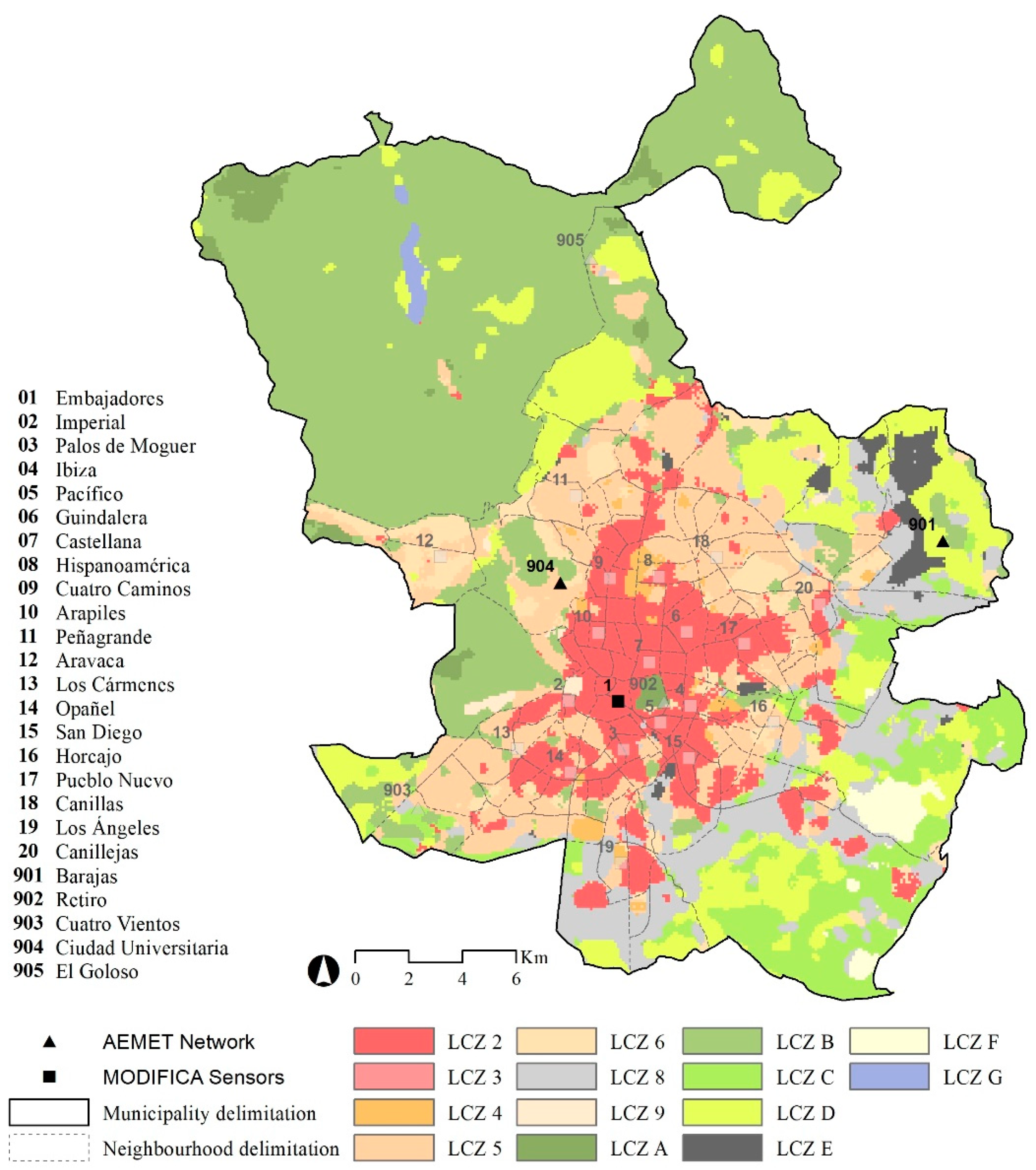
2.1. Study Area: The City of Madrid

The present study focuses on the city of Madrid. Due to its size, location and climatic conditions, Madrid is characterised by a strong UHI, with nighttime UHI intensities up to 10 °C during calm and clear nights. During the last decades, this phenomenon has been intensively studied in the city by means of on-site measurements [89,90,91,92], remote sensing [93,94] and numerical models [95,96].

Between 2016 and 2019, a continuous monitoring campaign was carried out at 20 fixed urban sites with the aim to study the temporal patterns of the UHI in Madrid [97]. In the present study, we use part of that experimental data to define the outputs of our ANN models. More specifically, we use the hourly, dry-bulb temperature gathered at the city centre (Embajadores, see Figure 1), classified as compact midrise (LCZ 2) according to the Local Climate Zones (LCZ) scheme [98], and which registered the highest mean and nighttime UHI intensity. The data available for this study cover the period from July 2016 to September 2018 on an hourly basis (800 days or 19,200 h, in total).

All sensors used in this monitoring campaign were protected from the rain and solar radiation using a custom-made, mechanically ventilated radiation shield. They were installed in the Urban Canopy Layer (UCL) at 5–6 m above the ground, following the guidelines of the World Meteorological Organization (WMO) for urban sites [99,100]. The location of each sensor was also studied in terms of its thermal source area [101]. In that sense, the representativeness of each sensor was appraised in terms of its surroundings’ homogeneity [102,103].

Quality Control (QC) procedures were also applied, consisting of a plausible value check, a time consistency check, and an internal-consistency check [104]. This analysis was complemented by a spatial consistency check [105], which analysed whether the difference between a measurement and its surroundings was too large compared to the average. For the City Centre sensor, 126 records were flagged as suspect and just three as erroneous. 72 missing values were identified due to a recording failure between the 17th and the 20th of October 2017. Both erroneous and missing values were left blank in the analysed dataset. Further details about the monitoring campaign and QC procedures can be found in [97].

In addition to the experimental data collected at the city centre, records from the nearby meteorological stations of Barajas Airport (LCZ D) and Ciudad Universitaria (LCZ 9) were used. Hourly values of dry bulb temperature, relative humidity, wind speed, wind direction and precipitation were extracted from the former, while global solar radiation was obtained from the latter. The data covered the same time period (July 2016–September 2018). Both stations are managed by the Spanish Meteorological Agency (AEMET), which complies with the requirements established by the WMO Integrated Global Observing System (WIGOS, [106,107]) regarding QC and sensor installation.

Three different types of datasets, the training, validation and the test datasets, were created. The former were used to fit and evaluate different ANN model configurations. Several training and validation datasets, which varied in length (12, 9, 6 and 3 months) and the months that they covered, were created based on almost 15 months of monitoring (July 2016–September 2017, 10,440 records/hourly measurements). All these datasets were continuous over time, and they were distributed as 80% training and 20% validation. These training and validation subsets were created by randomly sampling the data. This prevented the potential accumulation of specific events in any of these datasets (e.g., certain meteorological conditions), which could bias either the training or the validation of the models. Additionally, a test dataset was created based on the second year of recorded data (October 2017–September 2018, 8688 records/hourly measurements) to independently test the models and assess their accuracy over an entirely different year.

2.2. Designing the ANNs

Feed-forward Neural Networks (FNN) were used in this study. Although FNNs are at the baseline of supervised deep neural networks, their utility for modelling urban temperatures has been widely demonstrated in previous studies (see Section 1.1). Figure 2 outlines the two different approaches, based on two different outputs, that were adopted in this study to model urban temperatures. The first one consisted of directly targeting the air temperature at the urban site, validating its outputs with the measurements previously recorded at that location. This approach is aligned with the majority of similar studies found in the literature, and it is referred in this study as the temperature approach (TEMP approach). The second option aims at modelling the urban air temperature indirectly. In this case, the model targets the UHI intensity instead, computed as the temperature difference between the urban site (Embajadores) and the reference location (Barajas Airport, ΔT_{LCZ2, LCZD}). The urban temperature is then derived indirectly by adding the airport temperature to the output of the model. This will be referred to as the UHII approach from this point onwards.

The selection of the FNN model inputs of this study were informed by previous studies in Table 1, which have identified the variables that have a strong correlation with the formation of heat islands [109,110]. They consist of six meteorological variables: dry bulb temperature (°C), relative humidity (%), precipitation (mm), wind direction (degrees), wind speed (m/s) and global solar radiation (J/m²). The time of the day was added to these six input parameters, which was expected to reflect the daily variability of the outputs, either the temperature or the UHI intensity. Cloud cover was not used as an input parameter because the available frequency (one record every eight hours) was incompatible with the hourly frequency for the outputs. The wind speed presented strong variations at an hourly level and introduced strong oscillations in the prediction. Thus, to help avoid abrupt changes in the output, a moving average (MA) filter was applied. The use of a MA filter is a common pre-processing technique when it comes to modelling time series from data with a high variability. Examples can be found in the field of urban traffic (applying a MA to the car’s acceleration [111]), atmospheric pollution (MA applied to measured PM_2.5 concentration [112]) or urban climate modelling [113], the latter using a MA of order 8 (i.e., 8 h) to reduce the presence of wind gust peaks in the dataset prior feeding their model. In this study, a MA of order 4 (4 h) was found to be sufficient to reduce the noise of the wind speed while preserving the time series trend.

All the inputs were standardized prior the FNN feeding, meaning that all variables were transformed in order to have a mean = 0 and a standard deviation = 1 [114,115]. A diagram of the FNN structure for both approaches can be seen in Figure 3.

2.3. Comparing and Evaluating the FNNs

Several FNN structures with different configurations were trained during the first phase of this research. Hyperparameters, such as the number of neurons per hidden layer, the activation functions, or the number of epochs, were thoroughly iterated in order to find a common, optimal configuration for both the TEMP and the UHII approach. Despite some of the tested activation functions are commonly applied for classification tasks and were not likely to give the best performance (i.e., sigmoid-like functions), they were included in the iterative process since preceding similar works made use of them [24,67]. To streamline the process and reduce the complexity of the iteration, each subsequent hidden layer adopted half the neurons of the previous one. All models initialized their weights randomly and were initially trained using 12 months of data. Each configuration was compared by iterating just one parameter (e.g., the activation functions) and leaving the others fixed, while increasing the number of neurons per hidden layer. Those parameters that reached the best overall accuracy with the lowest number of neurons were selected. After this iterative process 5478 FNNs were trained.

Table 2. Parameters used to train and evaluate different FNNs configurations. It includes the configuration that was finally selected for both the temperature and the UHII approach.

Parameters		Tested	Selected
Number of hidden layers		1–5	2
Number of neurons	Input layer	7	7
	Hidden layers 1	3–85	18
	Output layer	1	1
Activation functions	Hidden layers	Linear, ELU, SELU, ReLU, Sigmoid, Hard sigmoid, Hyperbolic tangent, Exponential, Softmax, Softplus, Softsign	ELU
	Output layers	Linear, ELU, SELU, ReLU, Sigmoid, Hard sigmoid, Hyperbolic tangent, Exponential, Softmax, Softplus, Softsign	Linear
Optimizer		SGD, Adam, RMSProp, Adagrad, Adadelta, Nadam	Adam
Epochs		100, 200, 500	200
Batch size		2, 5, 10	10
Dataset length		12 months	12 months 2
Train/Validation size		80%/20%	80%/20%

¹ The value here presented corresponds to the number of neurons contained in the first hidden layer. Each subsequent hidden layer adopts half of the value of the previous one. ² Maximum length of the dataset. Results with shorter lengths are also presented (Table 4).

summarizes the parameters used to test these configurations, as well as the ones that were finally selected. The task outlined above was performed using Python and Keras, a deep-learning library based on Tensorflow [116,117].

Once a common structure and configuration were defined, a comparative analysis of these models was carried out. First, the contribution of each input to the model output was assessed using a sensitivity analysis [114,118,119]. The 5th, 25th, 50th, 75th and 95th percentiles were used to run the sensitivity analysis for each input, while fixing the rest on their means. The time of the day was excluded from the sensitivity analysis and fixed at two different moments: noon and midnight. Next, their overall accuracy was compared for the TEMP and the UHII approach using several error metrics, such as the root mean squared error (RMSE), the median absolute deviation (MAD) or the coefficient of determination (R²). Modelled results were then plotted for three different weeks to visually assess whether the modelling ability of any of these two approaches could be compromised under certain scenarios. These corresponded to a week of high atmospheric stability (and thus, strong UHI intensity), a week of high atmospheric instability (weak UHI intensity), and a week under both of these conditions.

The last step of the evaluation process consisted of modifying the amount of data provided to the neural networks during the training phase. To this end, FNN models for both the TEMP and the UHII approach were trained using 12, 9, 6 and 3 months of data, and were used to model the outdoor air temperatures for one complete year using the test dataset. The accuracy was estimated, as in the previous cases, using common error metrics. The loss of accuracy of the models trained with shorter datasets was addressed by comparing their performance with the models trained on more data, obtaining a percentage indicating the increase of error for each metric. In the case of models trained with just 3 months of data, the Mean Absolute Error (MAE) was estimated on a monthly basis to further explore its distribution along one year of modelling.

3. Results

A comparison between several FNN configurations is first shown in Figure 4. Each graph represents the overall accuracy of a certain FNN when iterating just one of its parameters, and while increasing the number of neurons in the hidden layers. From this iterative process, a common, optimal FNN configuration for both the TEMP and the UHII approach was established. The optimal structure was defined as a neural network with seven inputs, two hidden layers of 18 and 9 neurons respectively, and one output. In that sense, it was found that increasing from one to two hidden layers produced a significant improvement in the models’ accuracy, while increasing the number of hidden layers further did not. Similarly, moving from 100 to 200 epochs during the training phase could reduce the error of the FNN, while the computational expense of using 500 epochs instead of 200 did not seem justified. This was particularly evident when having tens of neurons in the hidden layers.

In some cases, due to the performance differences between the TEMP and the UHII approach, a common ground had to be reached in terms of the optimal configuration. That was the case of the activation functions, where the Stochastic Gradient Descent (SGD) seemed to produce the best results for those FNNs modelling the UHI intensity, but it led to exploding gradient problems when modelling the temperature. Thus, the Adaptive Moment Estimation (Adam) optimiser was used instead, which performed optimally in both scenarios. For the activation functions, a combination of the Exponential Linear Unit (ELU) for the hidden layers and the linear function for the output layer was used.

Overall, UHII models presented fewer converging problems than TEMP models, which seemed to have some difficulties with some activation functions and optimizers. Furthermore, the UHII approach usually outperformed the TEMP approach. The former did not only produce models with relatively smaller errors than the latter but required fewer neurons per hidden layer to reach a similar accuracy. This behaviour might be indicative of a clearer and more direct relationship between inputs and output, which in the case of the UHII approach links parameters such as wind speed, precipitation, or solar radiation with the UHI formation.

Differences between both modelling approaches also arise when looking at the inputs’ relevance. In that sense, the sensitivity analyses presented in Figure 5 and Figure 6 seem to reveal significant variations among them. The temperature from the reference site shifts from being the most relevant parameter of the entire FNN (TEMP approach) to being one of the least important (UHII approach). This is especially visible at night, when inter- and intra-urban temperature differences are most pronounced. The other parameters, albeit with different magnitude, seem to condition the outcome of both models in a similar way. In that sense, wind speed and direction seem to be two highly influential parameters during the night, while solar radiation and relative humidity seem to be key during the day.

Although the UHII approach appears to yield more balanced models, this apparent advantage does not seem to have a significant impact on their outputs when trained with 12 months of data. In this scenario, reasonably good results, and with similar error patterns, are obtained for both approaches. As it can be noted in Figure 7, modelled temperatures fit satisfactorily with the measured temperatures at the urban site and under a wide variety of circumstances, including different UHI scenarios: a rainy and windy week with generalised low UHI intensities (<2 °C); a week with varying meteorological conditions, during which a sudden weather change from calm to rainy was observed leading to a rapid change in the UHI intensities; or a calm week with strong UHI intensities (>5 °C), probably reinforced by temperature inversions.

The greatest errors seem to accumulate on those nights when unusual conditions occur, such as when very high UHI intensities, close to 10 °C, are registered; or when the UHI intensity drops and rises abruptly, perhaps coinciding with occasional and localised weather events, such as rainfalls. Overall, models produced relatively smooth time series, without spikes or large variations from one hour to the next one, despite not having a built-in temporal dependence between consecutive outputs. Using a moving average for the wind speed seems to have contributed to reducing the noise in the models’ output.

Models targeting the UHI intensity got a slightly better score in the error metrics, with a reduction of the error between 6.4 and 11.7% (see

Table 3. Metrics of the selected models targeting both the air temperature and the UHI intensity. Both models were trained using 12 months of data (July 2016–September 2017). The two variables regressed are modelled and monitored air temperatures.

Metrics		Model Targeting		Error Variation
		Temperature	UHI Intensity
MAD	Median Absolute Deviation (°C)	0.60	0.53	−11.7%
MAE	Mean Absolute Error (°C)	0.81	0.74	−8.6%
RMSE	Root Mean Squared Error (°C)	1.09	1.02	−6.4%
R2	Coefficient of Determination	0.99	0.79	+20.2%

). RMSE was 1.09 °C and 1.02 °C for the TEMP and the UHII approach, respectively. These results are in line with previous studies, such as in Kim and Baik (RMSE = 1.18 °C, [70]) or Demirezen et al. (RMSE = 1.29 °C, [75]), both modelling outdoor air temperature. The only exception is the coefficient of determination, which is extraordinarily high when targeting the temperature (R² = 0.99). This is also in line with previous studies (e.g., [75,77]) and it is further addressed in the discussion section.

Shortening the Training Dataset

The results presented above correspond to FNN models trained with one year of hourly data. So far, the TEMP and the UHII approach have proved to yield similar results. When training models with less data, however, differences started to arise. Results show that using 9 months instead of 12 months of data slightly increased the RMSE, with 0.9% and 2.4% for the TEMP and the UHII approach, respectively. When using 6 months of data the accuracy loss increased more markedly, especially in the case of the TEMP models (11.7% vs. 6.2%). The error kept growing exponentially when using 3 months of data, although the tendency was more accentuated and led to significant differences between both approaches (63.1% vs. 40.7%). A similar trend was observed for the MAE and MAD metrics, which can be found in

Table 4. Relative accuracy loss when reducing the size of the training dataset for both the TEMP and the UHII approach. The number of months in each column establish the baseline of accuracy. The accuracy was obtained using the evaluation dataset.

	TEMP Approach				UHII Approach
	RMSE				RMSE
	12 months	9 months	6 months	3 months	12 months	9 months	6 months	3 months
12 months	0.0%				0.0%
9 months	0.9%	0.0%			2.4%	0.0%
6 months	11.7%	10.6%	0.0%		6.2%	3.8%	0.0%
3 months	63.1%	61.6%	46.1%	0.0%	40.7%	37.5%	32.5%	0.0%
	MAE				MAE
	12 months	9 months	6 months	3 months	12 months	9 months	6 months	3 months
12 months	0.0%				0.0%
9 months	3.2%	0.0%			4.8%	0.0%
6 months	14.0%	10.4%	0.0%		8.9%	4.0%	0.0%
3 months	66.1%	60.9%	45.7%	0.0%	40.0%	33.7%	28.5%	0.0%
	MAD				MAD
	12 months	9 months	6 months	3 months	12 months	9 months	6 months	3 months
12 months	0.0%				0.0%
9 months	7.6%	0.0%			10.6%	0.0%
6 months	17.7%	9.4%	0.0%		14.5%	3.5%	0.0%
3 months	70.7%	58.7%	45.0%	0.0%	42.7%	29.0%	24.6%	0.0%

.

These results are the average error yielded by several models trained with shortened datasets and are relative to the accuracy of the models trained with 12 months of data. Figure 8 presents the models’ accuracy absolute levels, including the accuracy of all models trained with each shortened dataset. As already noted, differences arise not only when reducing the training datasets, but also when changing from one approach to another. The large variability of error between the models trained with 3 months of data is noticeable, being more accentuated in the case of the TEMP approach. It seems that, depending on the data used during training, it is possible to obtain models with an acceptable overall accuracy (RMSE < 1.5 °C, in line with previously developed models) to others that it is not clear that they could be used to make a reasonable modelling (RMSE > 2 °C).

Yet, these results represent the average cumulative error over a year. A more detailed analysis of the accuracy of the models showed that their error is unevenly distributed over the months, losing accuracy outside the months for which they were trained. It was also observed that their results do not suffer excessively within the months for which they were trained, being comparable with models trained on more data. In that sense, Figure 9 shows the additional error yielded by models trained with only 3 months of data. For convenience purposes, these months were made coincident with the seasons of the year, and a model trained with all 12 months of data was used as a reference.

The results show that the models systematically tend to minimise their error within their season, with the RMSE gradually increasing as they move away from it. This is accentuated for models trained in winter and summer. The reason behind this could lie in the annual cyclical behaviour of temperatures: between solstices and equinoxes, temperatures remain at one extreme of the annual cycle, either at the high end of temperatures (summer) or at the low end (winter). Between the equinoxes and solstices (spring and autumn), though, the transition between the two extremes takes place. This could favour the training of the ANN, as it would extend pattern recognition to practically the entire annual temperature range, and where only the extremes would be at the expense of the neural network’s ability to generalise and extrapolate its modelling capacity beyond what is known during its training.

This dynamic is noticeable in the case of the UHII approach as well, although it seems to be rather less pronounced. As it was pointed out in the introduction, Madrid’s UHI does not seem to follow a seasonal pattern, which means it might reach its highest and lowest UHII intensities at any time during the year (see Figure A1). However, these UHI peaks depend on the meteorological conditions, thus the loss of accuracy registered by these UHII models seems to be likely related to the concentration of certain meteorological conditions during the training phase. In other words, these FNNs would have difficulties in refining the modelling if, within the three months of data used to train them, there is not a sufficiently large record of the different meteorological conditions that favour the occurrence of UHI.

The performance differences between the TEMP and the UHII approach are now clearly noticeable when plotting the data. In this respect, Figure 10 shows how the results of a TEMP model trained from May to August would produce quite precise results for June of the next year, like the ones obtained by models trained with 12 months of data. However, when trying to obtain the temperature profile in February, that same model barely captures the global trend. In that scenario, the UHII model, trained with the same three months of data, was able to fit to observed values with higher accuracy. It accumulated the error at the same moment as the models trained with 12 months of data, in many cases amplifying it. Despite the unusual distribution of temperatures and UHI intensities for that week, the UHII model was able to capture most of it, which turned to be surprising due to the relatively low amount of data used for its training.

4. Discussion

The results of this research point towards the potential reduction of the training datasets without having a significant loss of accuracy. This could facilitate the work of urban climate researchers, thus promoting the development of shorter and simpler monitoring campaigns. This does not mean that it is preferable to use smaller amounts of data to train ANN models, but that their accuracy might not be compromised when they are trained in this manner. Although using large amounts of high-quality data is always desirable, in some cases it is not possible due to varying circumstances, such as budget constraints or human resources limitations. In this context, knowing where the accuracy limits of the models are when trained with fewer data might help researchers explore their experimental data or design new measurement campaigns in an efficient manner.

In this study we propose the use of empirical, FNN-based models to extend the temporal coverage of urban monitoring campaigns. These models, although limited for carrying out temporal predictions into the future, they can be used to adjust long-term records gathered outside the city to the urban context. This approach, the generation of long-term datasets by looking backwards, might be potentially useful in many disciplines, including the generation of site-specific weather files for building energy modelling [120,121,122,123], the downscaling of heat-related epidemiological studies to evaluate the effect of urban temperatures in health [4,124,125,126,127], or the identification and characterization of energy poor households in urban environments [128,129,130,131,132].

It is worth noting that the use of UHI intensity instead of outdoor temperature as the output of the FNN models yielded significantly better results mainly when reducing the size of the training dataset. The accuracy improvement was limited when using 9 or more months of data during the training phase. The benefits of targeting the UHI intensity with the FNN model are, therefore, linked to the potential of using smaller datasets to model outdoor urban temperatures. However, using the UHI intensity instead of the temperature as the output, sustained on the lower seasonality of the former, could be arguable. ANN are universal function approximators [133] and, for that reason, using one parameter or the other should not produce significant differences. Although this was mathematically demonstrated, Curry [134] showed that to model the seasonality of a time series with FNN would require a very large structure. This structure would grow exponentially when increasing the length of the dataset, since more turning points are likely to appear. In fact, Zhang and Qi [135] recommended not only to deseasonalize the time series, but also to remove its trend (if any). Nowadays, pre-processing the dataset to make it stationary before feeding the ANN is a very extended practice and has demonstrated to be very effective with RNN as well [88,136]. This approach might be helpful in the future for other studies such as Han et al. [86], where the UHI intensity could be used instead of the outdoor air temperature to remove much of the seasonality from their temperature forecasts. However, it is unclear whether they could be extended to FNNs that use a reference site for modelling outdoor urban temperatures without any time dependence. Other reasons, such as the range of temperatures or the concentration of meteorological stability of the training dataset, might explain the varying accuracy results between the TEMP and the UHII approach when training these types of models, especially when using just 3 months of training data.

In line with the latter, it seems that the selection of days with different meteorological conditions and at different times of the year might be more relevant for the modelling than the continuity of the monitoring campaign. Thus, it may be more appropriate that future studies work with shorter, discontinuous monitoring campaigns covering a wider range of meteorological situations rather than a single, continuous-over-time campaign that might concentrate in a specific time of the year. Results may also support the use of data from sources whose long-term continuity may be compromised (i.e., CWS). In these cases, it would be relevant not only to apply filtering techniques to reduce the risks of introducing outliers, but also to carry out frequency distribution analyses to ensure that all meteorological conditions are being included into the modelling.

Some attention should be drawn to the pertinence of using certain error metrics. Despite being very extended (e.g., [75,76,77]), the use of R² as a performance indicator could be misleading [137,138]. As it can be seen in Equation (1), R² relies both on the size of the residuals (SS_res, the actual deviation of the prediction from the observed values) and the total variance of the dependent variable (SS_tot):

$$R^2 = 1 - \frac{\sum {\left(y_i- {\widehat{y}}_i\right)}^2}{\sum {\left(y_i- {\overline{y}}_i\right)}^2} = 1 - \frac{S{S}_{res}}{S{S}_{tot}}$$

(1)

Thus, obtaining a higher R² does not implicitly mean having less error (numerator), but might be the result of a higher variance of the output (denominator). This was observed in this study when comparing the two approaches. In the case of the TEMP approach, the variance of the output temperature (which ranges from −2 to 41 °C) is much higher that the variance of the UHI intensity (ranging from 0 to 8 °C). Furthermore, since the TEMP approach contains an input variable (airport temperature) that explains most of the variance of the output variable (urban temperature), the R² tends to be extremely high (R² > 0.99). This explains why significantly lower R² were obtained when using the UHII approach in spite of yielding better results with the rest of the performance indicators (RMSE, MAE, MAD).

Taking the above into consideration, it would be worthwhile to investigate whether the behaviour of the TEMP and the UHII models presented in this paper is only attributable to the case of Madrid or if, on the contrary, it might be common in other cities at different latitudes and climatic conditions. Some existing studies have identified strong seasonal differences in UHI intensities in other cities [139,140,141,142], while others have not found such differences [143,144,145]. In this respect, a strong annual seasonality of the UHI intensity would probably limit the capacity of the models to produce accurate results when trained with small datasets. On the contrary, in cities where air temperatures remain within a narrow range throughout the year, such as tropical regions, the TEMP approach might perform better.

5. Conclusions

Feed-forward neural networks were used in this study to model urban temperature time series from experimental data. The aim was to explore the reliability of these models in the context of low data availability, as well as the potential benefits from targeting the UHI intensity with these models. Results showed that, for the case study of Madrid, the training dataset could be reduced to 9 or even 6 months without compromising too much the accuracy of the FNN models, particularly when using the UHII approach (2.4% and 6.2% increase in RMSE, respectively).

Results showed that the UHII approach generally outperformed the TEMP approach. Overall, UHII models converged to lower error ratios with a smaller number of neurons, proving to be more effective at predicting the urban temperature of a reference site. When using the exact same configuration and structure, UHII models exhibited a significant increase in performance. TEMP models appeared to be quite seasonally dependent, thus facing more problems for modelling temperatures outside the training months. This was particularly relevant when trained on just 3 months of data, when the accuracy differences between UHII and TEMP models was at their highest. We argue that this could be related to the annual cyclical behaviour of temperatures. Targeting the UHI intensity with the FNNs instead, which in Madrid has shown to be almost stationary, seems to reduce uncertainty when modelling temperatures from a relatively small dataset.

The potential use of smaller datasets for training FNNs and still obtaining reliable results might benefit urban climate researchers since field measurements could be reduced in time and costs. Researchers might also take advantage of the accurate preliminary results that can be generated with relatively small datasets for speeding up their research, or for extending their measurements to other urban areas.

References

1. Reckien, D.; Salvia, M.; Heidrich, O.; Church, J.M.; Pietrapertosa, F.; De Gregorio-Hurtado, S.; D’Alonzo, V.; Foley, A.; Simoes, S.G.; Krkoška Lorencová, E.; et al. How are cities planning to respond to climate change? Assessment of local climate plans from 885 cities in the EU-28. J. Clean. Prod. 2018, 191, 207–219. [Google Scholar] [CrossRef]
2. Santamouris, M.; Cartalis, C.; Synnefa, A. Local urban warming, possible impacts and a resilience plan to climate change for the historical center of Athens, Greece. Sustain. Cities Soc. 2015, 19, 281–291. [Google Scholar] [CrossRef]
3. Moran, D.; Kanemoto, K.; Jiborn, M.; Wood, R.; Többen, J.; Seto, K.C. Carbon footprints of 13,000 cities. Environ. Res. Lett. 2018, 13. [Google Scholar] [CrossRef]
4. Macintyre, H.; Heaviside, C.; Cai, X.; Phalkey, R. Comparing temperature-related mortality impacts of cool roofs in winter and summer in a highly urbanized European region for present and future climate. Environ. Int. 2021, 154, 106606. [Google Scholar] [CrossRef]
5. Sánchez-Guevara, C.; Núñez Peiró, M.; Taylor, J.; Mavrogianni, A.; Neila González, J. Assessing population vulnerability towards summer energy poverty: Case studies of Madrid and London. Energy Build. 2019, 190, 132–143. [Google Scholar] [CrossRef] [Green Version]
6. Hsu, A.; Sheriff, G.; Chakraborty, T.; Manya, D. Disproportionate exposure to urban heat island intensity across major US cities. Nat. Commun. 2021, 12, 2721. [Google Scholar] [CrossRef]
7. Grimm, N.B.; Faeth, S.H.; Golubiewski, N.E.; Redman, C.L.; Wu, J.; Bai, X.; Briggs, J.M. Global change and the ecology of cities. Science 2008, 319, 756–760. [Google Scholar] [CrossRef] [PubMed] [Green Version]
8. Youngsteadt, E.; Dale, A.G.; Terando, A.J.; Dunn, R.R.; Frank, S.D. Do cities simulate climate change? A comparison of herbivore response to urban and global warming. Glob. Chang. Biol. 2015, 21, 97–105. [Google Scholar] [CrossRef]
9. Blocken, B. Computational Fluid Dynamics for urban physics: Importance, scales, possibilities, limitations and ten tips and tricks towards accurate and reliable simulations. Build. Environ. 2015, 91, 219–245. [Google Scholar] [CrossRef] [Green Version]
10. Doan, V.Q.; Kusaka, H.; Nguyen, T.M. Roles of past, present, and future land use and anthropogenic heat release changes on urban heat island effects in Hanoi, Vietnam: Numerical experiments with a regional climate model. Sustain. Cities Soc. 2019, 47, 101479. [Google Scholar] [CrossRef]
11. Ampatzidis, P.; Kershaw, T. A review of the impact of blue space on the urban microclimate. Sci. Total Environ. 2020, 730, 139068. [Google Scholar] [CrossRef]
12. Boehme, P.; Berger, M.; Massier, T. Estimating the building based energy consumption as an anthropogenic contribution to urban heat islands. Sustain. Cities Soc. 2015, 19, 373–384. [Google Scholar] [CrossRef] [Green Version]
13. Best, M.J.; Grimmmmond, C.S.B. Key conclusions of the first international urban land surface model comparison project. Bull. Am. Meteorol. Soc. 2015, 96, 805–819. [Google Scholar] [CrossRef] [Green Version]
14. Jandaghian, Z.; Berardi, U. Comparing urban canopy models for microclimate simulations in Weather Research and Forecasting Models. Sustain. Cities Soc. 2020, 55, 102025. [Google Scholar] [CrossRef]
15. Chen, Y.; Zheng, B.; Hu, Y. Numerical simulation of Local Climate Zone cooling achieved through modification of trees, albedo and green roofs-a case study of Changsha, China. Sustainability 2020, 12, 2752. [Google Scholar] [CrossRef] [Green Version]
16. Tsoka, S.; Tsikaloudaki, A.; Theodosiou, T. Analyzing the ENVI-met microclimate model’s performance and assessing cool materials and urban vegetation applications—A review. Sustain. Cities Soc. 2018, 43, 55–76. [Google Scholar] [CrossRef]
17. Mirzaei, P.A. Recent challenges in modeling of urban heat island. Sustain. Cities Soc. 2015, 19, 200–206. [Google Scholar] [CrossRef] [Green Version]
18. Toparlar, Y.; Blocken, B.; Maiheu, B.; van Heijst, G.J.F. A review on the CFD analysis of urban microclimate. Renew. Sustain. Energy Rev. 2017, 80, 1613–1640. [Google Scholar] [CrossRef]
19. Lauzet, N.; Rodler, A.; Musy, M.; Azam, M.H.; Guernouti, S.; Mauree, D.; Colinart, T. How building energy models take the local climate into account in an urban context—A review. Renew. Sustain. Energy Rev. 2019, 116, 109390. [Google Scholar] [CrossRef]
20. Mirzaei, P.A.; Haghighat, F. Approaches to study Urban Heat Island—Abilities and limitations. Build. Environ. 2010, 45, 2192–2201. [Google Scholar] [CrossRef]
21. Stewart, I.D. Why should urban heat island researchers study history? Urban Clim. 2019, 30, 100484. [Google Scholar] [CrossRef]
22. Velasco, E. Go to field, look around, measure and then run models. Urban Clim. 2018, 24, 231–236. [Google Scholar] [CrossRef]
23. Muller, C.L.; Chapman, L.; Grimmond, C.S.B.; Young, D.T.; Cai, X. Sensors and the city: A review of urban meteorological networks. Int. J. Climatol. 2013, 33, 1585–1600. [Google Scholar] [CrossRef]
24. Gobakis, K.; Kolokotsa, D.; Synnefa, A.; Saliari, M.; Giannopoulou, K.; Santamouris, M. Development of a model for urban heat island prediction using neural network techniques. Sustain. Cities Soc. 2011, 1, 104–115. [Google Scholar] [CrossRef]
25. Giridharan, R.; Kolokotroni, M. Urban heat island characteristics in London during winter. Sol. Energy 2009, 83, 1668–1682. [Google Scholar] [CrossRef]
26. Kolokotroni, M.; Giridharan, R. Urban heat island intensity in London: An investigation of the impact of physical characteristics on changes in outdoor air temperature during summer. Sol. Energy 2008, 82, 986–998. [Google Scholar] [CrossRef] [Green Version]
27. Zhou, X.; Okaze, T.; Ren, C.; Cai, M.; Ishida, Y.; Watanabe, H.; Mochida, A. Evaluation of urban heat islands using local climate zones and the influence of sea-land breeze. Sustain. Cities Soc. 2020, 55, 102060. [Google Scholar] [CrossRef]
28. Skarbit, N.; Stewart, I.D.; Unger, J.; Gál, T. Employing an urban meteorological network to monitor air temperature conditions in the “local climate zones” of Szeged, Hungary. Int. J. Climatol. 2017, 37, 582–596. [Google Scholar] [CrossRef]
29. Chen, G.; He, M.; Li, N.; He, H.; Cai, Y.; Zheng, S. A method for selecting the typical days with full urban heat island development in hot and humid area, case study in Guangzhou, China. Sustainability 2021, 13, 320. [Google Scholar] [CrossRef]
30. Chao, C.C.; Hung, K.A.; Chen, S.Y.; Lin, F.Y.; Lin, T.P. Application of a high-density temperature measurement system for the management of the kaohsiung house project. Sustainability 2021, 13, 960. [Google Scholar] [CrossRef]
31. Borbora, J.; Das, A.K. Summertime Urban Heat Island study for Guwahati City, India. Sustain. Cities Soc. 2014, 11, 61–66. [Google Scholar] [CrossRef]
32. Beck, C.; Straub, A.; Breitner, S.; Cyrys, J.; Philipp, A.; Rathmann, J.; Schneider, A.; Wolf, K.; Jacobeit, J. Air temperature characteristics of local climate zones in the Augsburg urban area (Bavaria, southern Germany) under varying synoptic conditions. Urban Clim. 2018, 25, 152–166. [Google Scholar] [CrossRef]
33. Yang, X.; Yao, L.; Jin, T.; Peng, L.L.H.; Jiang, Z.; Hu, Z.; Ye, Y. Assessing the thermal behavior of different local climate zones in the Nanjing metropolis, China. Build. Environ. 2018, 137, 171–184. [Google Scholar] [CrossRef]
34. Yang, X.; Peng, L.L.H.; Chen, Y.; Yao, L.; Wang, Q. Air humidity characteristics of local climate zones: A three-year observational study in Nanjing. Build. Environ. 2020, 171, 106661. [Google Scholar] [CrossRef]
35. van der Heijden, M.G.M.; Blocken, B.; Hensen, J.L.M. Towards the integration of the urban heat island in building energy simulations. In Proceedings of the Building Simulation 2013: 13th Conference of the International Building Performance Simulation Association IBPSA, Chamberry, Ference, 25–28 August 2013; pp. 1006–1013. [Google Scholar]
36. Fenner, D.; Meier, F.; Scherer, D.; Polze, A. Spatial and temporal air temperature variability in Berlin, Germany, during the years 2001–2010. Urban Clim. 2014, 10, 308–331. [Google Scholar] [CrossRef]
37. Meier, F.; Fenner, D.; Grassmann, T.; Otto, M.; Scherer, D. Crowdsourcing air temperature from citizen weather stations for urban climate research. Urban Clim. 2017, 19, 170–191. [Google Scholar] [CrossRef]
38. Muller, C.L.; Chapman, L.; Johnston, S.; Kidd, C.; Illingworth, S.; Foody, G.; Overeem, A.; Leigh, R.R. Crowdsourcing for climate and atmospheric sciences: Current status and future potential. Int. J. Climatol. 2015, 35, 3185–3203. [Google Scholar] [CrossRef] [Green Version]
39. Fenner, D.; Meier, F.; Bechtel, B.; Otto, M.; Scherer, D. Intra and inter “local climate zone” variability of air temperature as observed by crowdsourced citizen weather stations in Berlin, Germany. Meteorol. Z. 2017, 26, 525–547. [Google Scholar] [CrossRef]
40. Nipen, T.N.; Seierstad, I.A.; Lussana, C.; Kristiansen, J.; Hov, Ø. Adopting citizen observations in operational weather prediction. Bull. Am. Meteorol. Soc. 2020, 101, E43–E57. [Google Scholar] [CrossRef]
41. Bell, S.; Cornford, D.; Bastin, L. How good are citizen weather stations? Addressing a biased opinion. Weather 2015, 70, 75–84. [Google Scholar] [CrossRef] [Green Version]
42. Chapman, L.; Bell, C.; Bell, S. Can the crowdsourcing data paradigm take atmospheric science to a new level? A case study of the urban heat island of London quantified using Netatmo weather stations. Int. J. Climatol. 2017, 37, 3597–3605. [Google Scholar] [CrossRef]
43. Kousis, I.; Pigliautile, I.; Pisello, A.L. Intra-urban microclimate investigation in urban heat island through a novel mobile monitoring system. Nat. Sci. Rep. 2021, 11, 9732. [Google Scholar] [CrossRef]
44. Yadav, N.; Sharma, C. Spatial variations of intra-city urban heat island in megacity Delhi. Sustain. Cities Soc. 2018, 37, 298–306. [Google Scholar] [CrossRef]
45. Schneider, R.; Taylor, J.; Davies, M.; Mavrogianni, A.; Milner, J.; Dos Santos, R.S.; Taylor, J.; Davies, M.; Mavrogianni, A.; Milner, J. The variation of air and surface temperatures in London within a 1 km grid using vehicle-transect and ASTER data. In Proceedings of the 2017 Joint Urban Remote Sensing Event, JURSE 2017, Dubai, United Arab Emirates, 6–8 March 2017; Institute of Electrical and Electronics Engineers Inc.: Manhattan, NY, USA, 2017; pp. 6–9. [Google Scholar]
46. Romero Rodríguez, L.; Sánchez Ramos, J.; Sánchez de la Flor, F.J.; Álvarez Domínguez, S. Analyzing the urban heat Island: Comprehensive methodology for data gathering and optimal design of mobile transects. Sustain. Cities Soc. 2020, 55, 102027. [Google Scholar] [CrossRef]
47. Heusinkveld, B.G.; Van Hove, L.W.A.; Jacobs, C.M.J.; Steeneveld, G.J.; El-Bers, J.A.; Moors, E.J.; Holtslag, A.A.M. Use of a mobile platform for assessing urban heat stress in Rotterdam. In Proceedings of the 7th Conference on Biometeorology, Freiburg, Germany, 12–14 April 2010; Volume 12, pp. 433–438. [Google Scholar]
48. Chow, W.T.L.; Pope, R.L.; Martin, C.A.; Brazel, A.J. Observing and modeling the nocturnal park cool island of an arid city: Horizontal and vertical impacts. Theor. Appl. Climatol. 2011, 103, 197–211. [Google Scholar] [CrossRef]
49. Brandsma, T.; Wolters, D. Measurement and statistical modeling of the urban heat island of the city of Utrecht (The Netherlands). J. Appl. Meteorol. Climatol. 2012, 51, 1046–1060. [Google Scholar] [CrossRef] [Green Version]
50. Fabbri, K.; Costanzo, V. Drone-assisted infrared thermography for calibration of outdoor microclimate simulation models. Sustain. Cities Soc. 2020, 52, 101855. [Google Scholar] [CrossRef]
51. Zhou, D.; Xiao, J.; Bonafoni, S.; Berger, C.; Deilami, K.; Zhou, Y.; Frolking, S.; Yao, R.; Qiao, Z.; Sobrino, J.A. Satellite remote sensing of surface urban heat islands: Progress, challenges, and perspectives. Remote Sens. 2019, 11, 48. [Google Scholar] [CrossRef] [Green Version]
52. László, E.; Szegedi, S. A multivariate linear regression model of mean maximum urban heat island: A case study of Beregszász (Berehove), Ukraine. Idojaras 2015, 119, 409–423. [Google Scholar]
53. Levermore, G.; Parkinson, J. The urban heat island of London, an empirical model. Build. Serv. Eng. Res. Technol. 2019, 40, 290–295. [Google Scholar] [CrossRef]
54. Levermore, G.J.; Parkinson, J.B. An empirical model for the urban heat island intensity for a site in Manchester. Build. Serv. Eng. Res. Technol. 2017, 38, 21–31. [Google Scholar] [CrossRef]
55. Romero Rodríguez, L.; Sánchez Ramos, J.; Molina Félix, J.L.; Álvarez Domínguez, S. Urban-scale air temperature estimation: Development of an empirical model based on mobile transects. Sustain. Cities Soc. 2020, 63, 102471. [Google Scholar] [CrossRef]
56. Bernard, J.; Musy, M.; Calmet, I.; Bocher, E.; Keravec, P. Urban heat island temporal and spatial variations: Empirical modeling from geographical and meteorological data. Build. Environ. 2017, 125, 423–438. [Google Scholar] [CrossRef] [Green Version]
57. Chun, B.; Guldmann, J.M. Spatial statistical analysis and simulation of the urban heat island in high-density central cities. Landsc. Urban Plan. 2014, 125, 76–88. [Google Scholar] [CrossRef]
58. Gardes, T.; Schoetter, R.; Hidalgo, J.; Long, N.; Marquès, E.; Masson, V. Statistical prediction of the nocturnal urban heat island intensity based on urban morphology and geographical factors—An investigation based on numerical model results for a large ensemble of French cities. Sci. Total Environ. 2020, 737, 139253. [Google Scholar] [CrossRef] [PubMed]
59. Jin, H.; Cui, P.; Wong, N.H.; Ignatius, M. Assessing the effects of urban morphology parameters on microclimate in Singapore to control the urban heat island effect. Sustainability 2018, 10, 206. [Google Scholar] [CrossRef] [Green Version]
60. Straub, A.; Berger, K.; Breitner, S.; Cyrys, J.; Geruschkat, U.; Jacobeit, J.; Kühlbach, B.; Kusch, T.; Philipp, A.; Schneider, A.; et al. Statistical modelling of spatial patterns of the urban heat island intensity in the urban environment of Augsburg, Germany. Urban Clim. 2019, 29, 100491. [Google Scholar] [CrossRef]
61. Chang, J.M.-H.; Lam, Y.F.; Lau, S.P.-W.; Wong, W.-K. Development of fine-scale spatiotemporal temperature forecast model with urban climatology and geomorphometry in Hong Kong. Urban Clim. 2021, 37, 100816. [Google Scholar] [CrossRef]
62. Ho, H.C.; Knudby, A.; Sirovyak, P.; Xu, Y.; Hodul, M.; Henderson, S.B. Mapping maximum urban air temperature on hot summer days. Remote Sens. Environ. 2014, 154, 38–45. [Google Scholar] [CrossRef]
63. Lai, J.; Zhan, W.; Quan, J.; Bechtel, B.; Wang, K.; Zhou, J.; Huang, F.; Chakraborty, T.; Liu, Z.; Lee, X. Statistical estimation of next-day nighttime surface urban heat islands. ISPRS J. Photogramm. Remote Sens. 2021, 176, 182–195. [Google Scholar] [CrossRef]
64. Zhou, J.; Zhou, J.; Chen, Y.; Wang, J.; Zhan, W.; Wang, J. Maximum Nighttime Urban Heat Island (UHI) Intensity Simulation by Integrating Remotely Sensed Data and Meteorological Observations. IEEE J. Sel. Top. Appl. Earth Obs. Remote Sens. 2011, 4, 138–146. [Google Scholar] [CrossRef]
65. Chen, Z.; Zhu, Z.; Jiang, H.; Sun, S. Estimating daily reference evapotranspiration based on limited meteorological data using deep learning and classical machine learning methods. J. Hydrol. 2020, 591, 125286. [Google Scholar] [CrossRef]
66. Venter, Z.S.; Brousse, O.; Esau, I.; Meier, F. Hyperlocal mapping of urban air temperature using remote sensing and crowdsourced weather data. Remote Sens. Environ. 2020, 242, 111791. [Google Scholar] [CrossRef]
67. Mihalakakou, G.; Santamouris, M.; Asimakopoulos, D. Modeling ambient air temperature time series using neural networks. J. Geophys. Res. 1998, 103, 19509–19517. [Google Scholar] [CrossRef]
68. Mihalakakou, G.; Flocas, H.A.; Santamouris, M.; Helmis, C.G. Application of Neural Networks to the Simulation of the Heat Island over Athens, Greece, Using Synoptic Types as a Predictor. J. Appl. Meteorol. 2002, 41, 519–527. [Google Scholar] [CrossRef]
69. Santamouris, M.; Mihalakakou, G.; Papanikolaou, N.; Asimakopoulos, D.N. A neural network approach for modeling the Heat Island phenomenon in urban areas during the summer period. Geophys. Res. Lett. 1999, 26, 337. [Google Scholar] [CrossRef]
70. Kim, Y.-H.; Baik, J.-J. Maximum Urban Heat Island Intensity in Seoul. J. Appl. Meteorol. 2002, 41, 651–659. [Google Scholar] [CrossRef]
71. Kolokotroni, M.; Davies, M.; Croxford, B.; Bhuiyan, S.; Mavrogianni, A. A validated methodology for the prediction of heating and cooling energy demand for buildings within the Urban Heat Island: Case-study of London. Sol. Energy 2010, 84, 2246–2255. [Google Scholar] [CrossRef] [Green Version]
72. Kolokotroni, M.; Zhang, Y.; Giridharan, R. Heating and cooling degree day prediction within the London urban heat island area. Build. Serv. Eng. Res. Technol. 2009, 30, 183–202. [Google Scholar] [CrossRef]
73. Kolokotroni, M.; Zhang, Y.; Watkins, R. The London Heat Island and building cooling design. Sol. Energy 2007, 81, 102–110. [Google Scholar] [CrossRef] [Green Version]
74. Demirezen, G.; Fung, A.S. Application of artificial neural network in the prediction of ambient temperature for a cloud-based smart dual fuel switching system. Energy Procedia 2019, 158, 3070–3075. [Google Scholar] [CrossRef]
75. Demirezen, G.; Fung, A.S.; Deprez, M. Development and optimization of artificial neural network algorithms for the prediction of building specific local temperature for HVAC control. Int. J. Energy Res. 2020, 44, 8513–8531. [Google Scholar] [CrossRef]
76. Papantoniou, S.; Kolokotsa, D. Prediction of outdoor air temperature using neural networks: Application in 4 European cities. Energy Build. 2016, 114, 72–79. [Google Scholar] [CrossRef]
77. Erdemir, D.; Ayata, T. Prediction of temperature decreasing on a green roof by using artificial neural network. Appl. Therm. Eng. 2017, 112, 1317–1325. [Google Scholar] [CrossRef]
78. Mihalakakou, G.; Santamouris, M.; Papanikolaou, N.; Cartalis, C.; Tsangrassoulis, A. Simulation of the Urban Heat Island Phenomenon in Mediterranean Climates. Pure Appl. Geophys. 2004, 161, 429–451. [Google Scholar] [CrossRef]
79. Jang, J.; Viau, A.A.; Anctil, F. Neural network estimation of air temperatures from AVHRR data. Int. J. Remote Sens. 2004, 25, 4541–4554. [Google Scholar] [CrossRef]
80. Zhao, D. Analysis of thermal environment and urban heat island using remotely sensed imagery over the north and south slope of the Qinling Mountain, China. In Proceedings of the 2007 IEEE International Geoscience and Remote Sensing Symposium, Barcelona, Spain, 23–27 July 2007; pp. 655–658. [Google Scholar]
81. Beccali, G.; Cellura, M.; Culotta, S.; Brano, V.L.; Marvuglia, A. A Web-Based Autonomous Weather Monitoring System of the Town of Palermo and Its Utilization for Temperature Nowcasting. In Computational Science and Its Applications—ICCSA 2008; Gervasi, O., Murgante, B., Laganà, A., Taniar, D., Mun, Y., Gavrilova, M.L., Eds.; Springer: Berlin, Germany, 2008; pp. 65–80. [Google Scholar]
82. Cellura, M.; Culotta, S.; Lo Brano, V.; Marvuglia, A.; Energetiche, R. Nonlinear Black-Box Models for Short-Term Forecasting of Air Temperature in the Town of Palermo. In Geocomputation, Sustainability and Environmental Planning; Murgante, B., Borruso, G., Lapucci, A., Eds.; Springer: Berlin, Germany, 2011; pp. 183–204. [Google Scholar]
83. Shao, B.; Zhang, M.; Mi, Q.; Xiang, N. Prediction and Visualization for Urban Heat Island. In Transactions on Edutainment VI. Lecture Notes in Computer Science, Volume 6758; Springer: Berlin, Germany, 2011; pp. 1–11. [Google Scholar]
84. Lee, Y.Y.; Kim, J.T.; Yun, G.Y. The neural network predictive model for heat island intensity in Seoul. Energy Build. 2016, 110, 353–361. [Google Scholar] [CrossRef]
85. Schuch, F.; Marpu, P.; Masri, D.; Afshari, A. Estimation of Urban Air Temperature from a Rural Station Using Remotely Sensed Thermal Infrared Data. Energy Procedia 2017, 143, 519–525. [Google Scholar] [CrossRef]
86. Han, J.M.; Ang, Y.Q.; Malkawi, A.; Samuelson, H.W. Using recurrent neural networks for localized weather prediction with combined use of public airport data and on-site measurements. Build. Environ. 2021, 192, 107601. [Google Scholar] [CrossRef]
87. ISO Online Browsing Platform. Available online: https://www.iso.org/obp/ui/#search (accessed on 14 January 2021).
88. Hewamalage, H.; Bergmeir, C.; Bandara, K. Recurrent Neural Networks for Time Series Forecasting: Current status and future directions. Int. J. Forecast. 2021, 37, 388–427. [Google Scholar] [CrossRef]
89. López Gómez, A.; López Gómez, J.; Fernández García, F.; Arroyo Ilera, F. El Clima Urbano de Madrid: La Isla de Calor; CSIC: Madrid, Spain, 1988; ISBN 978-84-00-07521-7.
90. Yagüe, C.; Zurita, E.; Martinez, A. Statistical analysis of the Madrid urban heat island. Atmos. Environ. 1991, 25, 327–332. [Google Scholar] [CrossRef]
91. Fernández García, F.; Montálvez, J.P.; González-Rouco, F.J.; Valero, F. A PCA Analysis of the UHI Form of Madrid. In Proceedings of the 5th International Conference on Urban Climate, Lodz, Poland, 1–5 September 2003; pp. 1–4. [Google Scholar]
92. Núñez Peiró, M.; Sánchez-Guevara Sánchez, C.; Neila González, F.J. Update of the Urban Heat Island of Madrid and Its Influence on the Building’s Energy Simulation; Springer: New York, NY, USA, 2017; ISBN 9783319514420. [Google Scholar]
93. López Gómez, A.; López Gómez, J.; Fernández García, F.; Moreno Jiménez, A. El Clima Urbano: Teledetección de la isla de Calor en Madrid; MOPT: Madrid, Spain, 1993; ISBN 978-84-00-07521-7. [Google Scholar]
94. Sobrino, J.A.; Oltra-Carrió, R.; Sòria, G.; Jiménez-Muñoz, J.C.; Franch, B.; Hidalgo, V.; Mattar, C.; Julien, Y.; Cuenca, J.; Romaguera, M.; et al. Evaluation of the surface urban heat island effect in the city of Madrid by thermal remote sensing. Int. J. Remote Sens. 2013, 34, 3177–3192. [Google Scholar] [CrossRef]
95. Salamanca, F.; Martilli, A. A new Building Energy Model coupled with an Urban Canopy Parameterization for urban climate simulations-part II. Validation with one dimension off-line simulations. Theor. Appl. Climatol. 2010, 99, 345–356. [Google Scholar] [CrossRef]
96. Salamanca, F.; Martilli, A.; Yagüe, C. A numerical study of the Urban Heat Island over Madrid during the DESIREX (2008) campaign with WRF and an evaluation of simple mitigation strategies. Int. J. Climatol. 2011, 32, 2372–2386. [Google Scholar] [CrossRef]
97. Núñez-Peiró, M.; Sánchez-Guevara Sánchez, C.; Neila González, F.J. Hourly evolution of intra-urban temperature variability across the local climate zones. The case of Madrid. Urban Clim. 2021, 39, 100921. [Google Scholar] [CrossRef]
98. Stewart, I.D.; Oke, T.R. Local climate zones for urban temperature studies. Bull. Am. Meteorol. Soc. 2012, 93, 1879–1900. [Google Scholar] [CrossRef]
99. Oke, T.R. Initial Guidance to Obtain Representative Meteorological Observations at Urban Sites (WMO/TD No. 1250); WMO: Geneva, Switzerland, 2006. [Google Scholar]
100. WMO. Guide to Meteorological Instruments and Methods of Observation (WMO No. 8); WMO: Geneva, Switzerland, 2017; Available online: http://www.posmet.ufv.br/wp-content/uploads/2016/09/MET-474-WMO-Guide.pdf (accessed on 15 July 2021).
101. Núñez Peiró, M.; Sánchez-Guevara Sánchez, C.; Neila González, F.J. Source area definition for local climate zones studies. A systematic review. Build. Environ. 2019, 148, 258–285. [Google Scholar] [CrossRef] [Green Version]
102. Alexander, P.J.; Bechtel, B.; Chow, W.T.L.; Fealy, R.; Mills, G. Linking urban climate classification with an urban energy and water budget model: Multi-site and multi-seasonal evaluation. Urban Clim. 2016, 17, 196–215. [Google Scholar] [CrossRef] [Green Version]
103. Kaplan, S.; Peeters, A.; Erell, E. Predicting air temperature simultaneously for multiple locations in an urban environment: A bottom up approach. Appl. Geogr. 2016, 76, 62–74. [Google Scholar] [CrossRef]
104. WMO. Guide to the Global Observing System (WMO No. 488); WMO: Geneva, Switzerland, 2017; Available online: https://library.wmo.int/doc_num.php?explnum_id=4236 (accessed on 15 July 2021).
105. Aguilar, E.; Auer, I.; Brunet, M.; Peterson, T.C.; Wieringa, J. Guidelines on Climate Metadata and Homogenization (WMO/TD No. 1186); WMO: Geneva, Switzerland, 2003; Available online: https://library.wmo.int/doc_num.php?explnum_id=9252 (accessed on 15 July 2021).
106. WMO. General Meteorological Standards and Recommended Practices (WMO No. 49); WMO: Geneva, Switzerland, 2018; Volume I, Available online: https://library.wmo.int/doc_num.php?explnum_id=10113 (accessed on 15 July 2021).
107. WMO. WIGOS Metadata Standard 2019; WMO: Geneva, Switzerland, 2019; Available online: https://library.wmo.int/doc_num.php?explnum_id=10109 (accessed on 15 July 2021).
108. Brousse, O.; Martilli, A.; Foley, M.; Mills, G.; Bechtel, B. WUDAPT, an efficient land use producing data tool for mesoscale models? Integration of urban LCZ in WRF over Madrid. Urban Clim. 2016, 17, 116–134. [Google Scholar] [CrossRef]
109. Oke, T.R.; Mills, G.; Christen, A.; Voogt, J.A. Urban Climates; Cambridge University Press: Cambridge, UK, 2017; ISBN 9781139016476. [Google Scholar]
110. Sundborg, A. Local Climatological Studies of the Temperature Conditions in an Urban Area. Tellus 1950, 2, 222–232. [Google Scholar] [CrossRef]
111. Zhou, M.; Qu, X.; Li, X. A recurrent neural network based microscopic car following model to predict traffic oscillation. Transp. Res. Part C Emerg. Technol. 2017, 84, 245–264. [Google Scholar] [CrossRef]
112. Shi, Y.; Ren, C.; Lau, K.K.L.; Ng, E. Investigating the influence of urban land use and landscape pattern on PM2.5 spatial variation using mobile monitoring and WUDAPT. Landsc. Urban Plan. 2019, 189, 15–26. [Google Scholar] [CrossRef]
113. Afshari, A.; Ramirez, N. Improving the accuracy of simplified urban canopy models for arid regions using site-specific prior information. Urban Clim. 2021, 35, 100722. [Google Scholar] [CrossRef]
114. Olden, J.D.; Jackson, D.A. Illuminating the “black box”: Understanding variable contributions in artificial neural networks. Ecol. Modell. 2002, 154, 135–150. [Google Scholar] [CrossRef]
115. Shanker, M.S.; Hu, M.Y.; Hung, M.S. Effect of data standardization on neural network training. Omega 1996, 24, 385–397. [Google Scholar] [CrossRef]
116. Abadi, M.; Barham, P.; Chen, J.; Chen, Z.; Davis, A.; Dean, J.; Devin, M.; Ghemawat, S.; Irving, G.; Isard, M.; et al. TensorFlow: A System for Large-Scale Machine Learning. In Proceedings of the 12th USENIX Symposium on Operating Systems Design and Implementation (OSDI’16), Savannah, GA, USA, 2–4 November 2016. [Google Scholar]
117. Chollet, F. Keras. Available online: https://keras.io (accessed on 28 February 2021).
118. Cortez, P.; Embrechts, M.J. Using sensitivity analysis and visualization techniques to open black box data mining models. Inf. Sci. 2013, 225, 1–17. [Google Scholar] [CrossRef] [Green Version]
119. Gerald, W.; Davis, J. Sensitivity Analysis in Neural Net Solutions. IEEE Trans. Syst. Man. Cybern. 1989, 19, 1078–1082. [Google Scholar] [CrossRef]
120. Ferrando, M.; Causone, F.; Hong, T.; Chen, Y. Urban building energy modeling (UBEM) tools: A state-of-the-art review of bottom-up physics-based approaches. Sustain. Cities Soc. 2020, 62, 102408. [Google Scholar] [CrossRef]
121. Erba, S.; Causone, F.; Armani, R. The effect of weather datasets on building energy simulation outputs. Energy Procedia 2017, 134, 545–554. [Google Scholar] [CrossRef]
122. Taylor, J.; Davies, M.; Mavrogianni, A.; Chalabi, Z.; Biddulph, P.; Oikonomou, E.; Das, P.; Jones, B. The relative importance of input weather data for indoor overheating risk assessment in dwellings. Build. Environ. 2014, 76, 81–91. [Google Scholar] [CrossRef]
123. Bienvenido-Huertas, D.; Marín-García, D.; Carretero-Ayuso, M.J.; Rodríguez-Jiménez, C.E. Climate classification for new and restored buildings in Andalusia: Analysing the current regulation and a new approach based on k-means. J. Build. Eng. 2021, 43, 102829. [Google Scholar] [CrossRef]
124. López-Bueno, J.A.; Linares, C.; Sánchez-Guevara, C.; Sánchez-Martínez, G.; Mirón, I.J.; Núñez Peiró, M.; Valero, I.; Díaz, J. The effect of cold waves on daily mortality in districts in Madrid considering sociodemographic variables. Sci. Total Environ. 2020, 749, 142364. [Google Scholar] [CrossRef] [PubMed]
125. López-Bueno, J.A.; Díaz, J.; Sánchez-Guevara, C.; Sánchez-Martínez, G.; Franco, M.; Gullón, P.; Núñez Peiró, M.; Valero, I.; Linares, C. The impact of heat waves on daily mortality in districts in Madrid: The effect of sociodemographic factors. Environ. Res. 2020, 190, 109993. [Google Scholar] [CrossRef] [PubMed]
126. López-Bueno, J.A.; Navas-martín, M.A.; Linares, C.; Mirón, I.J.; Luna, M.Y.; Sánchez-Martínez, G.; Culqui, D.; Díaz, J. Analysis of the impact of heat waves on daily mortality in urban and rural areas in Madrid. Environ. Res. 2021, 195, 110892. [Google Scholar] [CrossRef] [PubMed]
127. Macintyre, H.; Heaviside, C.; Cai, X.; Phalkey, R. The winter urban heat island: Impacts on cold-related mortality in a highly urbanized European region for present and future climate. Environ. Int. 2021, 154, 106530. [Google Scholar] [CrossRef] [PubMed]
128. Gouveia, J.P.; Seixas, J. Unraveling electricity consumption profiles in households through clusters: Combining smart meters and door-to-door surveys. Energy Build. 2016, 116, 666–676. [Google Scholar] [CrossRef]
129. Pino-Mejías, R.; Pérez-Fargallo, A.; Rubio-Bellido, C.; Pulido-Arcas, J.A. Artificial neural networks and linear regression prediction models for social housing allocation: Fuel Poverty Potential Risk Index. Energy 2018, 164, 627–641. [Google Scholar] [CrossRef]
130. Bienvenido-Huertas, D.; Pérez-Fargallo, A.; Alvarado-Amador, R.; Rubio-Bellido, C. Influence of climate on the creation of multilayer perceptrons to analyse the risk of fuel poverty. Energy Build. 2019, 198, 38–60. [Google Scholar] [CrossRef]
131. Serrano-Jiménez, A.; Lizana, J.; Molina-Huelva, M.; Barrios-Padura, Á. Indoor environmental quality in social housing with elderly occupants in Spain: Measurement results and retrofit opportunities. J. Build. Eng. 2020, 30, 101264. [Google Scholar] [CrossRef]
132. Castaño-Rosa, R.; Barrella, R.; Sánchez-Guevara, C.; Barbosa, R.; Kyprianou, I.; Paschalidou, E.; Thomaidis, N.S.; Dokupilova, D.; Gouveia, J.P.; Kádár, J.; et al. Cooling degree models and future energy demand in the residential sector. A seven-country case study. Sustainability 2021, 13, 2987. [Google Scholar] [CrossRef]
133. Hornik, K.; Stinchcombe, M.; White, H. Multilayer feedforward networks are universal approximators. Neural Netw. 1989, 2, 359–366. [Google Scholar] [CrossRef]
134. Curry, B. Neural networks and seasonality: Some technical considerations. Eur. J. Oper. Res. 2007, 179, 267–274. [Google Scholar] [CrossRef]
135. Zhang, G.P.; Qi, M. Neural network forecasting for seasonal and trend time series. Eur. J. Oper. Res. 2005, 160, 501–514. [Google Scholar] [CrossRef]
136. Bandara, K.; Bergmeir, C.; Smyl, S. Forecasting across time series databases using recurrent neural networks on groups of similar series: A clustering approach. Expert Syst. Appl. 2020, 140, 112896. [Google Scholar] [CrossRef] [Green Version]
137. Alexander, D.L.J.; Tropsha, A.; Winkler, D.A. Beware of R2: Simple, unambiguous assessment of the prediction accuracy of QSAR and QSPR models. J. Chem. Inf. Model. 2015, 55, 1316–1322. [Google Scholar] [CrossRef] [PubMed] [Green Version]
138. Kvalseth, T.O. Cautionary note about r2. Am. Stat. 1985, 39, 279–285. [Google Scholar] [CrossRef]
139. Roth, M. Review of urban climate research in (sub)tropical regions. Int. J. Climatol. 2007, 27, 1859–1873. [Google Scholar] [CrossRef]
140. Schwarz, N.; Lautenbach, S.; Seppelt, R. Exploring indicators for quantifying surface urban heat islands of European cities with MODIS land surface temperatures. Remote Sens. Environ. 2011, 115, 3175–3186. [Google Scholar] [CrossRef]
141. Suomi, J. Extreme temperature differences in the city of Lahti, southern Finland: Intensity, seasonality and environmental drivers. Weather Clim. Extrem. 2018, 19, 20–28. [Google Scholar] [CrossRef]
142. Zhou, B.; Rybski, D.; Kropp, J.P. On the statistics of urban heat island intensity. Geophys. Res. Lett. 2013, 40, 5486–5491. [Google Scholar] [CrossRef]
143. Fu, P.; Weng, Q. Variability in annual temperature cycle in the urban areas of the United States as revealed by MODIS imagery. ISPRS J. Photogramm. Remote Sens. 2018, 146, 65–73. [Google Scholar] [CrossRef]
144. Lazzarini, M.; Molini, A.; Marpu, P.R.; Ouarda, T.B.M.J.; Ghedira, H. Urban climate modifications in hot desert cities: The role of land cover, local climate, and seasonality. Geophys. Res. Lett. 2015, 42, 9980–9989. [Google Scholar] [CrossRef] [Green Version]
145. Zhou, B.; Lauwaet, D.; Hooyberghs, H.; De Ridder, K.; Kropp, J.P.; Rybski, D. Assessing Seasonality in the Surface Urban Heat Island of London. J. Appl. Meteorol. Climatol. 2016, 55, 493–505. [Google Scholar] [CrossRef] [Green Version]
Figure 1. Distribution of the MODIFICA and AEMET networks across the city of Madrid. The data needed for the training, validation and test of the ANN model was extracted from the measurement sites in black. The classification of Madrid by Local Climate Zones, extracted from the WUDAPT database [108], is presented in the background.
Sustainability 13 08143 g001
Figure 2. Schematic representation of the two approaches used for modelling the outdoor urban temperature.
Sustainability 13 08143 g002
Figure 3. Base structure of the Feed-forward Neural Network (FNN) used in this study.
Sustainability 13 08143 g003
Figure 4. Average Root Mean Squared Error for different FNN configurations using Table 2. Results obtained with the models derived from the TEMP and the UHII approach for the site Embajadores. Three weeks were selected, each one representing a different atmospheric stability scenario. The timeframe used to train these models extends from July 2016 to September 2017.
Sustainability 13 08143 g004
Figure 5. Sensitivity analysis of the inputs of the models. The same FNN configuration was used targeting the urban temperature (top) and the UHI intensity (bottom). The hour was fixed to 12 a.m. (Nighttime).
Sustainability 13 08143 g005
Figure 6. Sensitivity analysis of the inputs of the models. The same FNN configuration was used targeting the urban temperature (top) and the UHI intensity (bottom). The hour was fixed at 12 p.m. (Daytime).
Sustainability 13 08143 g006
Figure 7. Results obtained with the models derived from the TEMP and the UHII approach for the site Embajadores. Three weeks were selected, each one representing a different atmospheric stability scenario. The timeframe used to train these models extends from July 2016 to September 2017.
Sustainability 13 08143 g007
Figure 8. Comparison of the error obtained by several models, trained using different datasets of different length and differentiating between those targeting the air temperature and the UHI intensity. On the left is presented the RMSE. On the left is presented the RMSE. On the right is presented the MAD.
Sustainability 13 08143 g008
Figure 9. Additional error yielded by models trained with just 3 months of data, using both the TEMP and the UHII approach. These models are named according to the season they were trained on. The reference error baseline was established by the same ANN configuration trained with 12 months of data.
Sustainability 13 08143 g009
Figure 10. Comparison of TEMP and UHII models trained with 12 and 3 months of data for the site Embajadores. Results are presented for one week of June (top) and one week of February (bottom). The TEMP model trained on 3 months of data shows difficulties when modelling the temperatures further away from its training temporal range (i.e., February, bottom).
Sustainability 13 08143 g010