A Machine Learning-Based Prediction Model of LCCO₂ for Building Envelope Renovation in Taiwan

Abstract

In 2015, Taiwan’s government announced the “Greenhouse Gas Reduction and Management Act”, the goal of which was a 50% reduction in carbon emissions by 2050, compared with 2005. The residential and commercial sectors produce approximately one third of all carbon emissions in Taiwan, and the number of construction renovation projects is much larger than that of new construction projects. In this paper, we considered the life-cycle CO₂ (LCCO₂) of a building envelope renovation project in Tainan and focused on local construction methods for typical row houses. The LCCO₂ of 744 cases with various climate zones, orientations, and insulation and glazing types was calculated via EnergyPlus, SimaPro, and a local database (LCBA database), and the results were then used to develop a machine learning model. Our findings showed that the machine learning model was capable of predicting annual energy consumption and LCCO₂. With regard to annual energy consumption, the RMSE was 227.09 kW·h (per year) and the R² was 0.992. For LCCO₂, the RMSE was 2792.47 kgCO₂eq and the R² was 0.989, which indicates a high-confidence process for decision making in the early stages of building design and renovation.

1. Introduction

The increasing awareness of environmental protection has attracted global attention, with most industries taking the issue of sustainability seriously [1,2]. In 2015, countries around the world signed the Paris Agreement, which focuses primarily on reducing CO₂ and other greenhouse gas emissions [3]. Various countries have also promoted their own plans for carbon reduction strategies and green buildings [4,5,6,7,8,9,10].

In the United States, the Regional Greenhouse Gas Initiative (RGGI), established in 2009, was the first mandatory program to reduce greenhouse gas emissions. RGGI is a cooperative effort among certain states to limit and reduce CO₂ emissions from the power sector [11]. British Columbia, Canada, began implementing a carbon tax in 2008. As of 1 April 2021, B.C.’s carbon tax rate has been increased to $45 per tCO₂e (Canadian dollars) [12]. The Tokyo Metropolitan Government of Japan launched a green building program in 2002 to encourage energy saving technologies and environmentally friendly design in buildings [13]. The Tokyo Cap-and-Trade Program was launched in 2010 as the first mandatory carbon trading system in Japan. On aggregate, the emissions from 2015 to 2019 were reduced by 27% compared with base-year emissions [14].

In 2015, Taiwan’s government announced the “Greenhouse Gas Reduction and Management Act”, the goal of which was a 50% reduction in carbon emissions by 2050, compared with 2005. According to statistics from the International Energy Agency [15] and Environmental Protection Administration in Taiwan [16], Taiwan’s CO₂ emission from fuel combustion in 2018 was 257.0 MtCO₂, accounting for 0.77% of global emissions, and ranking 21st in the world. The average per capita emission is 10.83 tCO₂, ranking 20th in the world.

To achieve the goal of carbon reduction, the efforts of the building and construction industry are indispensable. Past studies have shown that the building and construction industry is responsible for 38% of all carbon emissions in the world and for about 35% of energy consumption [17]. The residential sector accounts for 11.49% of Taiwan’s total carbon emissions, mainly from electricity emissions such as air conditioners [18].

The development of the building and construction industry has clearly become a key factor in reducing global carbon emissions, with the proportion of construction renovation projects being much greater than that of new construction projects. Developing methods for providing a high-quality living environment in an energy-efficient, low-carbon way is a key factor in building renovations.

Many studies have pointed out that building envelopes have significant benefits regarding carbon reduction. Basbagill et al. [19] showed that the choice of building envelope has a great impact on carbon emissions during the life cycle of a building. The thermal insulation performance of windows and exterior walls influences the carbon emissions caused by urban household energy use. Therefore, high insulation performance can effectively alleviate heat in summer and cold in winter and thus further reduce household energy use [20].

We adopted life cycle assessment (LCA) to evaluate carbon emissions and costs. The LCA of buildings was used to assess the impact of buildings on the environment during their entire life cycle. The International Organization for Standardization (ISO) has developed a series of LCA-related standards [21,22], with the basic concept of evaluating the environmental impact of products in different life cycles (from cradle to grave). The scope includes the stages of raw material acquisition, manufacturing, use, and waste [23].

In the carbon footprint evaluation system for the building industry developed by the Low Carbon Building Alliance (LCBA) in Taiwan, the carbon footprint throughout all stages in the life cycle of a new building project includes the following five stages: manufacturing and transportation of materials; construction; daily use; renovation; and demolition. The life cycle for new building projects is generally defined as 60 years [24,25]. At present, almost all the carbon emissions of buildings in Taiwan are assessed using this system.

The carbon emissions of materials production are closely related to the local energy structure and energy efficiency. The carbon emission coefficients of different countries and regions vary. The use of the carbon emission database, which is calculated based on the local energy structure, is conducive to the accuracy of calculations. The LCBA carbon footprint database is also currently the most commonly used database in Taiwan’s building industry. According to standards of PAS2050 [26] and ISO 14,067 [27], the LCBA carbon footprint database integrates Taiwan’s existing construction engineering data and traces the carbon emissions data back to the raw materials.

Machine learning (ML) can solve specific problems or tasks through relative information and experiences and has been widely used in various prediction model studies, such as image and speech recognition [28,29], market analysis [30], etc. In the ML approach, a prediction model can be trained with input data to obtain the goal without solving theoretic equations.

ML has previously been used to predict the energy consumption of specific buildings: Robinson et al. [31] constructed predictive models for the energy consumption of commercial buildings in the United States using various ML methods; Ciulla et al. [32] used artificial neural networks to predict the demand for thermal energy linked to the winter acclimatization of non-residential buildings in Europe.

There has been less application of ML for prediction of carbon emissions than for energy consumption. A case study in Italy used an artificial neural network to predict building energy and various environmental indicators at the same time [33]. Reviewing the past literature, aside from there being fewer ML predictive models for carbon emissions, little discussion can be found on Taiwan’s climate and its architectural form, and very few scholars have studied the building renovation process.

Furthermore, several studies [34,35,36,37] have shown that the decision-making process to improve building energy efficiency often involves multiple criteria in addition to energy consumption and carbon emissions. A multi-purpose optimization system can assist designers in decision-making during the design or renovation process.

As stated above, accurate calculations and simulation of building energy consumption and carbon emissions are time-consuming and laborious. The purpose of this research is to use ML methods to develop a model for predicting energy consumption and carbon emissions based on Taiwan’s climate and common building patterns. The results can be used to quickly evaluate the sustainability of a building in the initial stage of architectural design or the renovation phase.

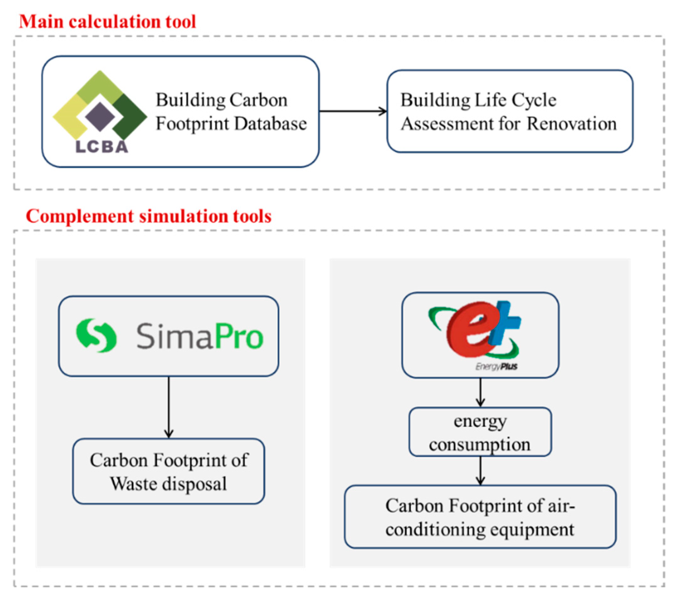
This study considered the LCCO₂ of a building envelope renovation project in Taiwan and studied the local construction methods for typical row houses. Through EnergyPlus, SimaPro, and the local database (LCBA database), the annual energy consumption and the LCCO₂ of 744 cases with various climate zones, orientations, insulation types, and glazing types were calculated, and the results were used to develop an ML model.

In Section 2, we introduce the methodology, which is mainly divided into data collection and ML training processes. Section 3 explains the results, including data observation, the results of adjusting hyperparameters, and the final prediction model, and Section 4 presents the conclusion.

2. Materials and Methods

The entire workflow is shown in Figure 1. We first defined the research object and confirmed the scope of variables. Then the life cycle of CO₂ (LCCO₂) and annual energy consumption of each case was calculated to generate the dataset required for ML. After-wards, model training and final performance evaluation were performed. We divided the remaining explanation of our methods into two subsections to describe the collection and generation of the dataset and then the ML training process.

2.1. Data Collection

2.1.1. Research Object

Excluding the Taipei metropolitan area, row houses accounted for the highest proportion of all residential types in Taiwan with 49.02% [38]. As a result, this study takes reinforced concrete row houses as the object of simulation analysis to reflect the current situation of Taiwan’s housing types (Figure 2,

Table 1. Basic setting conditions of space.

Space	Size
Living room	1104 cm × 470 cm × 400 cm
Main bedroom	500 cm × 470 cm × 300 cm
Bedroom	300 cm × 470 cm × 300 cm

). The variables of this study consisted of the replacement of partial materials (roof/exterior wall/glass) so that ML could be used in the initial design or renovation phase. The building information is as follows:

• Building scale: 4.7 m × 11.03 m;
• Floor area: 127.06 m²;
• Surface area: roof is 51.88 m², exterior wall is 123 m², glass is 20 m²;
• Three-story row house;
• First floor is living room and kitchen, whose height is 4 m, with a 2.5 m × 1 m window at the front and a 3.5 m × 1 m window at the rear;
• Second and third floors are bedrooms with the same plan, whose height is 3 m, with 3.5 m × 1 m windows at the front and rear.

The roof, exterior wall, and glass were set according to the common structure of existing row houses in Taiwan. The construction settings are shown in

Table 2. Cases of roof construction methods.

Case Number of Roof	Construction Method	U Value (W/m2∙K)
R0	Coating material	2.68
R1	Foam concrete	0.82
R2	Foam concrete + flexible heat insulating material	1.00
R3	Five-foot insulation brick	0.84
R4	Flexible heat insulating material + coating material	0.77
R5	Cement mortar + rigid heat insulating material	0.75
R6	Face brick	1.06
R7	Cool roof coating	2.60
R8	Wooden plank roof	0.94
R9	Foam concrete (thickening) + flexible heat insulating material	0.97
R10	Flexible heat insulating material (thickening) + coating material	0.70
R11	Cement mortar + rigid heat insulating material (thickening)	0.46

,

Table 3. Cases of exterior wall construction methods.

Case Number of Wall	Construction Method	U Value (W/m2∙K)
W0	Tiling wall	3.13
W1	Coating material	3.2
W2	Dry construction for stone	1.3
W3	Coating material + heat insulating material	0.82
W4	Wet construction for stone	3.17
W5	Wet construction for stone (thickening)	3.14
W6	Rustic or washed finish	3.17

and

Table 4. Cases of glass materials and construction methods.

Case Number of Glass	Glass Type		Thickness (mm)	U Value (W/m2∙K)	SHGC	Visible Transmittance
G0	Single glass	plate glass	3	5.9	0.87	0.90
G1		plate glass	6	6.16	0.82	0.91
G2		plate glass	12	5.88	0.75	0.92
G3		on-line Low-E glass	6	6.16	0.62	0.91
G4		on-line Low-E glass	12	5.88	0.54	0.91
G5		on-line reflecting glass	6	6.16	0.48	0.6
G6		off-line reflecting glass	6	6.16	0.25	0.63
G7	Laminated glass	plate glass	6 + pvb + 6	4.88	0.73	0.9
G8		on-line reflecting glass	6 + pvb + 6	4.88	0.5	0.64
G9		off-line reflecting glass	6 + pvb + 6	4.88	0.23	0.64
G10	Double-layered glass	plate glass	6 + air + 6	3.23	0.73	0.86
G11		on-line reflecting glass	6 + air + 6	3.23	0.4	0.69
G12		off-line reflecting glass	6 + air + 6	3.23	0.18	0.63
G13		on-line Low-E glass	6 + air + 6	3.23	0.53	0.88
G14		off-line (single silver coating) Low-E glass	6 + air + 6	3.23	0.57	0.85
G15		off-line (double silver coating) Low-E glass	6 + air + 6	3.23	0.46	0.88

. Four orientations (east, west, south, and north) are used to represent the characteristics of houses with different orientations to expand the applicability of the simulation. Furthermore, each case is simulated in three climate zones (Northern, Central, and Southern Taiwan). The representative points are Taipei, Taichung, and Kaohsiung. The basic data of weather stations are shown in

Table 5. Basic data of representative weather stations.

Climate Zone	Weather Station	Longitude	Latitude	Altitude
Northern Taiwan	Taipei	121.5° E	25.0° N	6.3 m
Central Taiwan	Taichung	120.7° E	24.1° N	84 m
Southern Taiwan	Kaohsiung	120.3° E	22.6° N	2.3 m

.

2.1.2. Method of Data Collection

• Life-Cycle CO₂

The LCCO₂ assessment of this study is primarily based on the LCBA system and focuses on the carbon footprint of building renovation, including the related material carbon footprint and the influence of air conditioning energy consumption during the use phase. The life cycle of a renovation building project is defined as 20 years.

The calculation items involved in the building renovation project are shown in Figure 3, including material consumption and energy, but only the energy consumption of air conditioning equipment is calculated in the use phase. The calculation of LCCO₂ in this study, as shown in Equation (1), is divided into four main parts: building renovation materials, renovation construction phase (including demolition of the original structure), use phase of air conditioning electricity, and waste disposal phase.

The relevant tools for calculation are shown in Figure 4. In the use phase and disposal phase, other simulation tools were used as supplements for further calculation.

The calculation of the carbon emissions of air conditioning during the use phase converts the results of energy consumption according to the carbon emission coefficient announced by the Ministry of Economic Affairs [39]. The annual energy consumption is given by the simulation result of air conditioning energy consumption with EnergyPlus and is then converted into the carbon emissions of the use phase over 20 years (life cycle of a renovation building project). The simulation settings of EnergyPlus are explained in Section 2.2.2.

Regarding waste disposal, since the LCBA database is still lacking in this regard, the SimaPro database is used to make up for its shortcomings. SimaPro is a calculation software commonly used for LCA analysis worldwide. The software uses its detailed database to calculate the environmental impact of a product, from raw material production to the final processing stage, by modeling the production process of the product.

$$\mathrm{TCF}=\mathrm{CFdw}+\mathrm{CFm}+\mathrm{CFc}+\mathrm{CFa}.$$

(1)

• TCFL: CCO₂ of a renovation building project (kgCO₂eq)
• CFdw: Carbon footprint of waste disposal (kgCO₂eq)
• CFm: Carbon footprint of materials (kgCO₂eq)
• CFc: Carbon footprint of construction (kgCO₂eq)
• CFa: Carbon footprint of air conditioning (kgCO₂eq)

2.

Energy

EnergyPlus is a building energy simulation software jointly developed by the US Department of Energy, Lawrence Berkeley National Laboratory, US Construction Engineering Research Laboratory, Oklahoma State University, the University of Illinois, and other institutions. It can be used to conduct a comprehensive energy consumption simulation analysis of a building’s heating load, lighting, ventilation, and energy consumption of other equipment [40]. It has become a widespread and accepted tool for both academic and commercial uses in building energy analysis around the world [41].

The calculation of building energy consumption is closely related to external weather conditions. In the simulations, the weather data of Typical Meteorological Years (TMY3) are usually used. This study uses the TMY3 developed by the Architecture and Building Research Institute of Taiwan to simulate the indoor heating load of the building. These data adopted the Sandia Method developed by the National Renewable Energy Laboratory of the United States (NREL) as a standard method for constructing TMY3 and the raw weather data recorded by the Central Weather Bureau from 1990 to 2012 [42]. Three elements of TMY3 were extracted as the features of the subsequent ML process (

Table 6. Model training features of TMY3.

Weather Station	Annual Average of Dry Bulb Temperature	Annual Average of Relative Humidity	Annual Average of Wind Speed
Taipei	23.3 °C	78%	2.4 m/s
Taichung	23.8 °C	75.5%	1.48 m/s
Kaohsiung	25.5 °C	76.8%	2.18 m/s

).

Under the premise that the original design of the building remains unchanged, we replaced the building materials, with the exception of the main structure, according to the common structure of Taiwan’s existing row houses as mentioned in Section 2.1. Among them, the short side of the exterior wall is the street-facing facade, and the simulation was set to be affected by airflow and sunlight. Meanwhile, the wall connected to the neighboring house (the long side of the exterior wall) was set as an insulating wall during simulation. Indoor floors, doors, and walls were not affected by airflow and sunlight.

The setting of indoor temperature and the ventilation method are shown in

Table 7. Simulation setting of indoor temperature and ventilation method.

Indoor Temperature	Relationship between Indoor and Outdoor Temperature	Ventilation Method
>26 °C	-	Close the windows and turn on the air conditioner
<26 °C	outdoor temperature > indoor temperature	Close the windows
	outdoor temperature < indoor temperature	Open the windows for natural ventilation

. The Coefficient of Performance (COP) was set to 4.5. The discharge coefficient for the opening factor was set to 0.6 when the window was open and 0.0001 when the window was closed.

2.2. Machine Learning

This study adopted the supervised learning method, which uses data with known results for training for the purpose of predicting data with unknown results. The gradient boosting decision tree (GBDT) algorithm was used to construct the model. The GBDT is an algorithm of ensemble learning that combines the gradient descending and boosting and uses the decision tree as the basic learner. The concept of gradient boosting was derived from the observations of Leo Breiman and was further developed by Friedman [43].

Gradient descending is a commonly used optimization algorithm for finding the local minimum by calculating the gradient and moving in the opposite direction. Boosting can generate a strong learner from an ensemble of weak learners, each of which can barely do better than random guessing [44]. The process of boosting involves building a model, then increasing the weight of data that are incorrectly predicted by this model to create a second model, and repeating the same steps to obtain a better-performing model.

In GBDT, a sequence of decision trees (weak learners of GBDT) uses gradient descending to reduce the loss of the model with each step. While the first decision tree is built using the original predictor, every subsequent tree is built with the loss calculated from the predicted value of the previous tree and the target value, so that the final loss approaches zero.

The proportions of the training and testing sets were 80% and 20%, respectively. We further used a cross-validation method (K-fold cross-validation, K = 10) to reduce the problem of overfitting and adjusted the hyperparameters to improve the model performance. The whole process was implemented with python (version 3.6.8), using the library Scikit-learn (version 0.22.2.post1) as the main ML tool [45].

2.2.1. Performance Evaluation

In the data observation part, the Spearman rank correlation coefficient was used to observe the correlation between the variables. Root mean square error (RMSE), percentage error, and R² were used to evaluate the performance of the trained model. These values are defined as follows:

$$\mathrm{RMSE}=\sqrt{\frac{1}{N}\sum {\left({y^{\prime }}_i-y_i\right)}^2}$$

(2)

$$\mathrm{percentage}\mathrm{error}=\frac{{y^{\prime }}_i-y_i}{y_i}\times 100\%$$

(3)

$$R^2=\frac{\sum {\left({y^{\prime }}_i-\overline{y}\right)}^2}{\sum {\left(y_i-\overline{y}\right)}^2}$$

(4)

where N is the number of samples, $y_i$ is real values, ${y^{\prime }}_i$ is predicted values, and $\overline{y}$ is the mean of real values.

2.2.2. Dataset for Model Training

The variables of the database used in this study consisted of 11 columns and 744 rows. Input features included three climatic conditions, one azimuth condition, and five material conditions. The predicted targets were annual energy consumption and LCCO₂ of the renovation life cycle. The columns are represented in

Table 8. List of variables for dataset.

		Range	Code	Unit
Input features	Annual average of dry bulb temperature	23.3–25.5	temperature_avg	°C
	Annual average of relative humidity	75.5–78.0	RH_avg	%
	Annual average of wind speed	1.48–2.40	speed_avg	m/s
	Orientation	0–360	orientation	°
	U value of roof	0.46–2.68	roof U	W/m2∙K
	U value of exterior wall	0.82–3.20	wall U	W/m2∙K
	U value of glass	3.23–6.16	glass U	W/m2∙K
	Solar heat gain coefficient of glass	0.18–0.87	glass SHGC	-
	Visible transmittance of glass	0.60–0.92	glass VT	-
Output targets	Annual energy consumption	4159–16,788	energy	kWh
	Building life cycle carbon footprint for renovation	50,647–181,853	LCCO2	kgCO2eq

, and the distribution of each variable is shown in Figure 5 and Figure 6.

3. Results and Discussion

3.1. Data Observation and Feature Selection

The correlation map (Figure 7) shows that the correlation coefficient between annual energy consumption and LCCO₂ is quite high. It is speculated that daily use (air conditioning) accounts for the largest portion of the entire renovation life cycle, thus establishing a strong positive correlation with annual energy consumption. Furthermore, the relationship with the location is also very close, particularly the temperature, while humidity and wind speed also have some influence.

As for the correlation coefficient of materials, the U values of the exterior walls and roofs have a relatively weak relationship with annual energy consumption and LCCO₂. It is speculated that under the climate of Taiwan, the main heat enters through the windows in the form of radiation and causes the indoor temperature to rise, thus increasing the heat that needs to be removed. Therefore, the U value is not in a dominant position.

However, the correlation coefficient only considers the linear relationship between the two variables. A strong correlation does not necessarily mean a causal relationship. Moreover, the additive effect caused by other variables besides the two variables cannot be presented.

This study tried two combinations of features to compare the accuracy of their predictions. The input features are shown in

Table 9. Input features of each model.

Model_1	Model_2
1. temperature_avg	1. temperature_avg
2. RH_avg	2. RH_avg
3. speed_avg	3. speed_avg
4. orientation	4. orientation
5. roof U	5. glass U
6. wall U	6. glass SHGC
7. glass U
8. glass SHGC

. Model_1 had all the features in the dataset, a total of eight variables. Model_2 deleted features with low correlation from the correlation map. Figure 8 shows the distribution of percentage error. It can be seen that the model in which the U values of the exterior wall and roof were deleted does not perform as well as the model that used all the features.

3.2. Tuning the Hyperparameters

The two hyperparameters of the GBDT model were adjusted, namely n_estimators and max_depth. The remaining hyperparameters were set to default values. The n_estimators represents the number of boosting stages to perform, that is, the total number of decision trees created in the model. In general, the larger the value, the better the performance of the model, but after reaching a certain number, the performance of the model will not increase significantly. The max_depth represents the maximum depth of each decision tree and limits the number of nodes in the tree. The best value depends on the interaction of the input variables [33].

Appropriate hyperparameters were selected based on the RMSE of the model and the time spent, as shown in Figure 9 and Figure 10. In n_estimators, the larger the value, the more time it takes, but the trend of model performance improvement in the later period slows down. Ultimately, n_estimators = 960 was selected. The larger the max_depth is, the RMSE of the training set decreases significantly, but the RMSE of the validation set increases after max_depth > 3. The phenomenon of overfitting indicates that the model is too complex. Although it can fit the training data well, it has poor applicability to unseen data (poor generalization ability). Therefore, we selected a max_depth value of 3 in the final model.

3.3. Results of Machine Learning Model

3.3.1. Annual Energy Consumption

In terms of predicting annual energy consumption, the GBDT model shows quite high accuracy. The scatter plot and box plot (Figure 11 and Figure 12) show that, despite some outliers, most of the data are consistent with the dataset.

Table 10. Model performance of annual energy consumption.

	RMSE	R2
Training set	191.65 kWh	0.994
Testing set	227.09 kWh	0.992

shows the RMSE and R² of the training and testing sets. The R² is greater than 0.99. The performance of the model is excellent, and the training set does not differ much from the testing set, which means that the model has not caused too much overfitting, and its predictive ability on unseen data has a certain degree of credibility.

3.3.2. Building Life-Cycle Carbon Footprint for Renovation

The prediction of building life-cycle carbon footprint for renovation also has high accuracy (Figure 13 and Figure 14). Although its accuracy is slightly lower than the performance of annual energy consumption, the performance of the overall data still has a certain predictive power.

Table 11. Model performance of LCCO₂.

	RMSE	R2
Training set	2288.81 kgCO2eq	0.993
Testing set	2792.47 kgCO2eq	0.989

shows its RMSE and R².

In the prediction model for annual energy consumption and LCCO₂ in this study, we used the same input variables. In addition to the extremely high correlation between the two, it also considers the availability of data in practice. The input variables currently used are all easily obtainable material properties. With such data, it is a good result for predicting building renovation LCCO₂.

4. Conclusions

In this study, our goal was to use ML to predict the annual energy consumption and life-cycle carbon footprint of row houses in Taiwan for the renovation behavior of buildings. In terms of applicability, only simple material properties and climatic conditions needed to be input; in terms of model performance, it had high accuracy.

Therefore, compared with the current technologies generally used, which usually require the building of a 3D model and need detailed material properties to obtain accurate energy consumption and carbon emissions, when using the ML model developed in this research, as long as one enters the eight features listed in Table 9, one can obtain the predicted annual energy consumption and LCCO₂ of a row house in a very short time.

Such a simple and fast ML predictive model can also be integrated into a mul-ti-purpose optimized system in the future to assist designers in decision-making. Usually, the targets involved in building design optimization are complicated, very time-consuming, or need to set many parameters. Integrating the ML model into the op-timization system is convenient to use and has practical applications.

Before performing supervised learning, a credible database for training was necessary. Therefore, this study used the LCBA database, the most commonly used carbon emission database in Taiwan’s building industry, and complemented it with the SimaPro database to calculate building carbon emissions. Furthermore, since different materials cause different energy consumption in the subsequent use phase, we used EnergyPlus to determine the annual energy consumption of air conditioning in each case to obtain more accurate life-cycle carbon emissions results.

Regarding the construction of ML models, selecting the best features is important. Even a low correlation with the target does not mean that the variable has no effect on the ML model. Our results show that even though the importance of features can be preliminarily determined from the correlation map, this only represents the relationship between the two parameters. In the ML model, various parameters may interact with each other and then affect the final prediction result. Therefore, when adjusting the input features of the model, more detailed comparisons and judgments are needed to obtain more suitable input features.

The generalization of ML depends on the dataset used, so the model constructed in this study can only be used to predict the form of row houses. However, the ML model thus constructed does not have to be limited to row houses in Taiwan. If the dataset is expanded to cover different building types, it may become a more flexible and extensive predictive model in the future.

Furthermore, our discussion was only focused on the three representative climate zones of Taiwan. If data on different cities can be added in the future, the scope of application can be expanded. Regarding the selection of materials, since this study adopts the most common structural form in Taiwan, the distribution of U values is somewhat too concentrated, especially with regard to the exterior wall, and whether it will cause problems in the prediction of exterior walls of other structures remains to be studied.

In summary, if the number and diversity of sample data can be increased, the scope of application of prediction models can be continuously expanded. However, with regard to the common renovation behavior of row houses in Taiwan, the prediction model proposed by this study can effectively predict the annual energy consumption and building life-cycle carbon footprint quickly and conveniently.

References

1. Mebratu, D. Sustainability and Sustainable Development: Historical and Conceptual Review. Environ. Impact Assess. Rev. 1998, 18, 493–520. [Google Scholar] [CrossRef]
2. Gasparatos, A.; El-Haram, M.; Horner, M. A Critical Review of Reductionist Approaches for Assessing the Progress towards Sustainability. Environ. Impact Assess. Rev. 2008, 28, 286–311. [Google Scholar] [CrossRef]
3. United Nations Framework Convention on Climate Change (UNFCCC), Paris Agreement. Available online: https://unfccc.int/sites/default/files/english_paris_agreement.pdf (accessed on 12 May 2021).
4. Lu, M.; Lai, J. Review on Carbon Emissions of Commercial Buildings. Renew. Sustain. Energy Rev. 2020, 119, 109545. [Google Scholar] [CrossRef]
5. Kauffmann, C.; Less, C.T.; Teichmann, D. Corporate Greenhouse Gas Emission Reporting. OECD Work. Pap. Int. Invest. 2012. [Google Scholar] [CrossRef]
6. Wallhagen, M.; Glaumann, M.; Malmqvist, T. Basic Building Life Cycle Calculations to Decrease Contribution to Climate Change—Case Study on an Office Building in Sweden. Build. Environ. 2011, 46, 1863–1871. [Google Scholar] [CrossRef]
7. Jeong, K.; Hong, T.; Kim, J. Development of a CO2 Emission Benchmark for Achieving the National CO2 Emission Reduction Target by 2030. Energy Build. 2018, 158, 86–94. [Google Scholar] [CrossRef]
8. Lai, J.H.K. Mandatory Reporting of Greenhouse Gas Emissions from Buildings: Stakeholders’ Opinions in Hong Kong. Energy Policy 2014, 75, 278–288. [Google Scholar] [CrossRef]
9. Jiang, P.; Chen, Y.; Dong, W.; Huang, B. Promoting Low Carbon Sustainability through Benchmarking the Energy Performance in Public Buildings in China. Urban Clim. 2014, 10, 92–104. [Google Scholar] [CrossRef]
10. Martin, C. Generating Low-Cost National Energy Benchmarks: A Case Study in Commercial Buildings in Cape Town, South Africa. Energy Build. 2013, 64, 26–31. [Google Scholar] [CrossRef]
11. Regional Greenhouse Gas Initiative (RGGI). The Regional Greenhouse Gas Initiative and Initiative of the Northeast and Mid-Atlantic States of the U.S. Available online: https://www.rggi.org/ (accessed on 12 May 2021).
12. Government of British Columbia, British Columbia’s Carbon Tax. Available online: https://www2.gov.bc.ca/gov/content/environment/climate-change/planning-and-action/carbon-tax (accessed on 12 May 2021).
13. Japan Bureau of Environment, Green Building Program. Available online: https://www.kankyo.metro.tokyo.lg.jp/en/climate/build.html (accessed on 12 May 2021).
14. International Carbon Action Partnership, Japan-Tokyo Cap-and-Trade Program. Available online: https://icapcarbonaction.com/en/?option=com_etsmap&task=export&format=pdf&layout=list&systems%5B%5D=51 (accessed on 12 May 2021).
15. International Energy Agency (IEA). Key World Energy Statistics 2020. Available online: https://iea.blob.core.windows.net/assets/1b7781df-5c93-492a-acd6-01fc90388b0f/Key_World_Energy_Statistics_2020.pdf (accessed on 12 May 2021).
16. Environmental Protection Administration Executive Yuan, R.O.C (Taiwan). Greenhouse Gas Emission Statistics. Available online: https://www.epa.gov.tw/Page/81825C40725F211C/6a1ad12a-4903-4b78-b246-8709e7f00c2b (accessed on 12 May 2021)(In Traditional Chinese).
17. United Nations Environment Programme. 2020 Global Status Report for Buildings and Construction: Towards a Zero-Emission, Efficient and Resilient Buildings and Construction Sector. Available online: https://globalabc.org/news/launched-2020-global-status-report-buildings-and-construction (accessed on 12 May 2021).
18. Ministry of the Interior, R.O.C (Taiwan). Greenhouse Gas Emission Control Action Plan in Residential and Commercial Sectors. Available online: https://escs.cdri.org.tw/?page_id=117 (accessed on 12 May 2021). (In Traditional Chinese).
19. Basbagill, J.; Flager, F.; Lepech, M.; Fischer, M. Application of Life-Cycle Assessment to Early Stage Building Design for Reduced Embodied Environmental Impacts. Build. Environ. 2013, 60, 81–92. [Google Scholar] [CrossRef]
20. Ye, H.; Wang, K.; Zhao, X.; Chen, F.; Li, X.; Pan, L. Relationship between Construction Characteristics and Carbon Emissions from Urban Household Operational Energy Usage. Energy Build. 2011, 43, 147–152. [Google Scholar] [CrossRef]
21. ISO 14040:2006—Environmental Management—Life Cycle Assessment—Principles and Framework; International Organization for Standardization: Geneva, Switzerland, 2006.
22. ISO 14044:2006—Environmental Management—Life Cycle Assessment—Requirements and Guidelines; International Organization for Standardization: Geneva, Switzerland, 2006.
23. Fenner, A.E.; Kibert, C.J.; Woo, J.; Morque, S.; Razkenari, M.; Hakim, H.; Lu, X. The Carbon Footprint of Buildings: A Review of Methodologies and Applications. Renew. Sustain. Energy Rev. 2018, 94, 1142–1152. [Google Scholar] [CrossRef]
24. Lin, H.-T. Carbon Footprint of the Building Industry: Carbon Management Strategies for Buildings, Landscapes, and Interior Decoration, 3rd ed.; Chan’s Arch-Publishing: Taipei, Taiwan, 2018; (In Traditional Chinese). [Google Scholar]
25. Lin, H.-T. Carbon footprint evaluation & certification system for the building industry–building, landscaping and interior renovation in Taiwan. In Proceedings of the Grand Renewable Energy Proceedings Japan Council for Renewable Energy, Yokohama, Japan, 20–22 June 2018; p. 94. [Google Scholar]
26. PAS 2050:2008—Specification for the Assessment of the Life Cycle Greenhouse Gas Emissions of Goods and Services; British Standards Institution: London, UK, 2008.
27. ISO/TS 14067:2013—Greenhouse Gases—Carbon Footprint of Products—Requirements and Guidelines for Quantification and Communication; International Organization for Standardization: Geneva, Switzerland, 2013.
28. Ciregan, D.; Meier, U.; Schmidhuber, J. Multi-Column Deep Neural Networks for Image Classification. In Proceedings of the IEEE Computer Society Conference on Computer Vision and Pattern Recognition, Long Beach, CA, USA, 16–22 June 2012; pp. 3642–3649. [Google Scholar]
29. Hinton, G.; Deng, L.; Yu, D.; Dahl, G.; Mohamed, A.R.; Jaitly, N.; Senior, A.; Vanhoucke, V.; Nguyen, P.; Sainath, T.; et al. Deep Neural Networks for Acoustic Modeling in Speech Recognition: The Shared Views of Four Research Groups. IEEE Signal Process. Mag. 2012, 29, 82–97. [Google Scholar] [CrossRef]
30. Patel, J.; Shah, S.; Thakkar, P.; Kotecha, K. Predicting Stock and Stock Price Index Movement Using Trend Deterministic Data Preparation and Machine Learning Techniques. Expert Syst. Appl. 2015, 42, 259–268. [Google Scholar] [CrossRef]
31. Robinson, C.; Dilkina, B.; Hubbs, J.; Zhang, W.; Guhathakurta, S.; Brown, M.A.; Pendyala, R.M. Machine Learning Approaches for Estimating Commercial Building Energy Consumption. Appl. Energy 2017, 208, 889–904. [Google Scholar] [CrossRef]
32. Ciulla, G.; D’Amico, A.; Lo Brano, V.; Traverso, M. Application of Optimized Artificial Intelligence Algorithm to Evaluate the Heating Energy Demand of Non-Residential Buildings at European Level. Energy 2019, 176, 380–391. [Google Scholar] [CrossRef]
33. D’Amico, A.; Ciulla, G.; Traverso, M.; Lo Brano, V.; Palumbo, E. Artificial Neural Networks to Assess Energy and Environmental Performance of Buildings: An Italian Case Study. J. Clean. Prod. 2019, 239, 117993. [Google Scholar] [CrossRef]
34. Carli, R.; Dotoli, M.; Pellegrino, R.; Ranieri, L. Using Multi-Objective Optimization for the Integrated Energy Efficiency Improvement of a Smart City Public Buildings’ Portfolio. IEEE Int. Conf. Autom. Sci. Eng. 2015, 2015, 21–26. [Google Scholar] [CrossRef]
35. Diakaki, C.; Grigoroudis, E.; Kabelis, N.; Kolokotsa, D.; Kalaitzakis, K.; Stavrakakis, G. A Multi-Objective Decision Model for the Improvement of Energy Efficiency in Buildings. Energy 2010, 35, 5483–5496. [Google Scholar] [CrossRef]
36. Jaggs, M.; Palmer, J. Energy Performance Indoor Environmental Quality Retrofit—A European Diagnosis and Decision Making Method for Building Refurbishment. Energy Build. 2000, 31, 97–101. [Google Scholar] [CrossRef]
37. Kaklauskas, A.; Zavadskas, E.K.; Raslanas, S. Multivariant Design and Multiple Criteria Analysis of Building Refurbishments. Energy Build. 2005, 37, 361–372. [Google Scholar] [CrossRef]
38. Construction and Planning Agency, MOI, R.O.C (Taiwan). Sampling Survey of Housing Conditions in 2015; Construction and Planning Agency, MOI, R.O.C (Taiwan): Taipei, Taiwan, 2015; (In Traditional Chinese). [Google Scholar]
39. Ministry of Economic Affairs, R.O.C (Taiwan). 2019 Electricity Carbon Emission Coefficient. Available online: https://ghgregistry.epa.gov.tw/Upload/News3/00001330_001.pdf (accessed on 30 January 2021)(In Traditional Chinese).
40. Crawley, D.B.; Lawrie, L.K.; Winkelmann, F.C.; Buhl, W.F.; Huang, Y.J.; Pedersen, C.O.; Strand, R.K.; Liesen, R.J.; Fisher, D.E.; Witte, M.J.; et al. EnergyPlus: Creating a New-Generation Building Energy Simulation Program. Energy Build. 2001, 33, 319–331. [Google Scholar] [CrossRef]
41. Stadler, M.; Firestone, R.; Curtil, D.; Marnay, C. On-Site Generation Simulation with EnergyPlus for Commercial Buildings; Lawrence Berkeley National Laboratory: Berkeley, CA, USA, 2006. [Google Scholar]
42. Architecture and Building Research Institute, Ministry of the Interior, R.O.C (Taiwan). The Development and Research on Hourly Typical Meteorological Years (TMY3) for Building Energy Simulation Analysis of Taiwan; Architecture and Building Research Institute, Ministry of the Interior, R.O.C (Taiwan): Taipei, Taiwan, 2020; (In Traditional Chinese). [Google Scholar]
43. Friedman, J.H. Greedy Function Approximation: A Gradient Boosting Machine. Ann. Stat. 2001, 29, 1189–1232. [Google Scholar] [CrossRef]
44. Zhang, C.; Ma, Y. (Eds.) Ensemble Machine Learning: Methods and Applications; Springer: Boston, MA, USA, 2012; ISBN 1441993258. [Google Scholar]
45. Documentation of Scikit-Learn 0.22.2. Available online: https://scikit-learn.org/0.22/index.html (accessed on 25 February 2021).
Figure 1. Workflow of this research.
Sustainability 13 08209 g001
Figure 2. Illustration of row house. (a) Perspective; (b) plan.
Sustainability 13 08209 g002
Figure 3. Renovation process and calculation scope of carbon emissions.
Sustainability 13 08209 g003
Figure 4. Calculation tools for carbon emissions.
Sustainability 13 08209 g004
Figure 5. Distribution of input features for dataset.
Sustainability 13 08209 g005
Figure 6. Distribution of output features for dataset.
Sustainability 13 08209 g006
Figure 7. Spearman’s rank correlation map of data features.
Sustainability 13 08209 g007
Figure 8. Distribution of percentage error of each model. (a) Annual energy consumption; (b) LCCO2 for renovation.
Sustainability 13 08209 g008
Figure 9. Tuning the hyperparameter for annual energy consumption. (a) n_estimators; (b) max_depth.
Sustainability 13 08209 g009
Figure 10. Tuning the hyperparameter for LCCO2. (a) n_estimators; (b) max_depth.
Sustainability 13 08209 g010
Figure 11. Model prediction of annual energy consumption for training set. (a) Scatter plot; (b) box plot.
Sustainability 13 08209 g011
Figure 12. Model prediction of annual energy consumption for testing set. (a) Scatter plot; (b) box plot.
Sustainability 13 08209 g012
Figure 13. Model prediction of LCCO2 for training set. (a) Scatter plot; (b) box plot.
Sustainability 13 08209 g013
Figure 14. Model prediction of LCCO2 for testing set. (a) Scatter plot; (b) box plot.
Sustainability 13 08209 g014