Abstract
The increase of greenhouse gases emission, global warming, and even climate change is an ongoing issue. Sustainable logistics and distribution management can help reduce greenhouse gases emission and lighten its influence against our living environment. Quantum computing has become more and more popular in recent years for advancing artificial intelligence into the next generation. Hence, we apply quantum random number generator to provide true random numbers for the genetic algorithm to solve the pollution-routing problems (PRPs) in sustainable logistics management in this paper. The objective of the PRPs is to minimize carbon dioxide emissions, following one of the seventeen sustainable development goals set by the United Nations. We developed a two-phase hybrid model combining a modified k-means algorithm as a clustering method and a genetic algorithm with quantum random number generator as an optimization engine to solve the PRPs aiming to minimize the pollution produced by trucks traveling along delivery routes. We also compared the computation performance with another hybrid model by using a different optimization engine, i.e., the tabu search algorithm. From the experimental results, we found that both hybrid models can provide good solution quality for CO2 emission minimization for 29 PRPs out of a total of 30 instances (30 runs each for all problems).
1. Introduction
Global warming and climate change are ongoing issues right now and required immediate attention around the world (Figure 1). Climate change and global warming are related to the emission of greenhouse gases into the atmosphere, theoretically. One of the important observations during the global pandemic of the new coronavirus (COVID-19) is that many regions have been on lockdown for several months. The aerosols and pollutants in the atmosphere reduced by around 9–64% [1]. It is obvious that human activities have a significant influence on the amount of pollutants in the atmosphere. Therefore, methods for reducing greenhouse gases emission in daily life and industries has become an important issue. Inefficient logistics and distribution management will produce more greenhouse gases emission, since trucks need to travel for a longer time and consume more fuel. Globalized enterprises need to pay more attention and take action to green their supply chain [2].
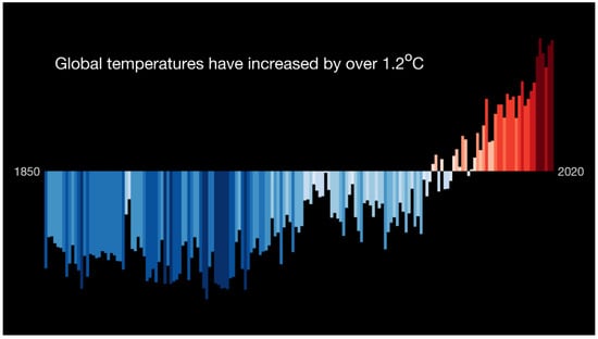
Figure 1.
Global warming bar chart (source: Institute for Environmental Analytics).
With continuous development of the vehicle routing problems (VRPs), various types of VRPs have been proposed for more than 60 years of time [3,4,5,6]. Among them, the pollution-routing problems (PRPs) and green vehicle routing problems (GVRPs) are directly related to one of the seventeen sustainable development goals set by the United Nations.
The PRPs were first proposed in 2011 by the authors of [7]. They extended classical VRPs with broader and more comprehensive objective functions that considered not only the travel distance, but also the amount of greenhouse gases emission, fuel consumption, travel times, and their costs. They also reminded that the amount of pollution emitted by trucks depends on their load and speed, along with other factors. Later, the variants of the PRP attracted many researchers. The authors of [8] extended the PRP into a dual objectives model in 2014. The authors of [9] added time-dependent constraints into the PRP, as the time-dependent PRP model in 2017. The authors of [10] extended the PRP into a continuous model and solved the continuous PRP.
Almost within the same period, the GVRPs were introduced in 2012 by the authors of [11]. They formulated the GVRPs and developed some solution techniques to help organizations with alternative fuel-powered vehicle (AFV) fleets overcome the difficulties that currently limit vehicle driving range and limited refueling infrastructure.
The VRPs and its variants are NP-hard (non-deterministic polynomial-time hardness) problems. Various methods and algorithms have been proposed and tested to optimize solutions, according to the objectives for each problem. Meta-heuristic methods have been widely applied to solve the problems, including traditional genetic algorithms (GA), Tabu searches (TS), simulated annealing (SA), neighborhood searches, [12,13] etc. However, some algorithms may have better results when applied to certain problems, compared to others; determining which method is the best algorithm to solve the VRPs is still argued in research/academic society. Therefore, we designed and compared the different results by utilizing two different optimization algorithms, the GA with quantum random number generator (QRNG) and the TS, as part of the hybrid models to solve the PRPs in this paper. Moreover, we execute grouping techniques before optimizing to design our hybrid models in order to cluster customer points, based on their demands in the first phase. The objective was to develop hybrid models to solve the PRPs in a short time, whether in small-scale problems or large-scale problems, by combining clustering algorithms and optimization algorithms into integrated models.
The GA was first developed by the author of [14], which is inspired by the concept of “natural selection and survival of the fittest” proposed by Darwin’s theory of evolution. The construction of the GA included chromosome selection, gene reproduction, crossover, and mutation. The original concept was to mimic the biological chromosomal gene architecture to represent complex system structures. Generally, when the GA is used to solve problems, the principles of genetic evolution are mainly used for searching for better solutions. Since the GA was proposed, many studies have used it to solve the VRPs and their variants [15,16,17].
The concept of the TS was first introduced in 1986 by the author of [18] to solve integer programming problem and serve as linkage to artificial intelligence at the beginning of personal computer era. The author of [19] proposed theory of the TS in 1990 and the TS was designed to enable searching process to escape local optimal and go to global optimal. The TS is based on introducing flexible memory structures, combined with strategic restrictions and aspiration levels, as a means for exploiting search spaces. This method is typically used in combinatorial optimization, such as travelling salesman problems (TSPs), manufacture scheduling problems, VRPs [20,21,22], etc. The overall approach is to avoid entrapment in cycles by forbidding or penalizing moves which take the solution, in the next iteration, to points in the solution space previously visited. This property is one of the important reasons why the TS can get satisfying solutions efficiently.
With the development of quantum mechanics, applications of quantum technology have been more valued in recent years by powerful quantum computers. Following Industry 4.0 by using artificial intelligence in a smart factory, the potential of quantum technology with artificial intelligence in the future is shown in Figure 2. Quantum computing was introduced by the author of [23]. It is the use of quantum phenomena, such as superposition and entanglement, to perform computation. Quantum superposition states that any two or more quantum states can be added together, and the result will be another valid quantum state. Also, quantum entanglement is a phenomenon where a pair of particles are generated and interact or share spatial proximity, in such a way that the quantum state of each particle of the pair cannot be described independently of the state of the other, even when the distance between the particles is large.
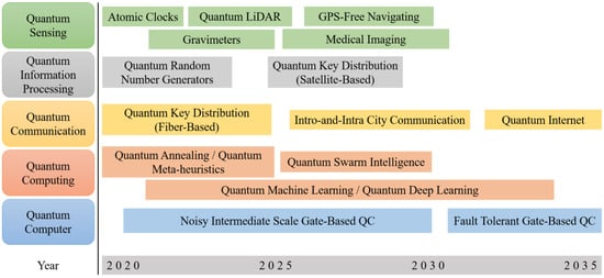
Figure 2.
Quantum technology timeline.
Quantum computers are believed to be able to solve certain computational problems and calculate faster than classical computers, and that is the reason why more and more researchers began to study from data science to quantum information science.
Random numbers, which have important applications in simulation and cryptography, are a fundamental resource in science and engineering. However, the random number generators that we usually use have certain complicated rules or functions to generate outputs by inputting certain seeds, called the pseudo-random number generator (PRNG). The QRNG can provide truly random numbers because of the inherent randomness at the core of quantum mechanics, thus making quantum systems a perfect source of entropy. Also, the QRNG is one of the most mature quantum technologies [24], and the optical QRNG is a popular type of the QRNG [25,26]. The QRNG we embedded in our proposed hybrid model was acquired from the Australian National University QRNG server (https://qrng.anu.edu.au/ (accessed on 30 March 2021)).
The research objective focused on the business model of Business to Customers. In addition, we proposed two hybrid models and compared two different optimization engines: the GA with QRNG (GAQ), and the TS, to solve the PRPs.
The assumptions and limitations within the research are listed as follows:
- Each route started and ended at the same depot. Depots had all the required demands from customers.
- Product categories were not considered in this research.
- Each customer was visited exactly once by a truck and had known inhomogeneous demands; additionally, the service time was closed to 0.
- The location of each customer was known in advance.
- Every truck had the same known capacity. The total demand of each route did not exceed the truck capacity.
- There was no limit to the number of places that each truck could visit, nor the total duration of each route.
- No time-variant factory (no midnight delivery) or event occurrence could disrupt delivery.
- Every truck had the same weight, 3000 kg, when it was empty. The weight of every unit of demand was 100 kg.
- The distance, per unit, in the plane coordinates was 1 km.
- The basic fuel consumption of each vehicle was 6.25 L per 100 km. The fuel consumption increased linearly by 0.5 L per 100 km (for every 100 kg of additional vehicle weight). Every liter of fuel consumed produced 2.2 kg of CO2.
Under all the stated assumptions and limitations, trying to search for the minimum total emission of CO2 during the delivery was the research objective. The parameters in the assumptions could easily be changed (either increased or reduced) in the real world by computer software simulation.
2. Research Methodology
2.1. Problem Proposition
The PRPs in this research considered a single depot with a capacity constraint for each truck. The objective of the PRP was to minimize the total emission of CO2 during the delivery. The PRP was represented by a directed graph: G = (V, E), where V = {v0, …, vn} implied the set of nodes and E was the set of arcs. Typically, the depot was denoted with node j = 0, and customers were denoted with j = 1, 2, …, N, where N was the last customer that needed to be served. The demand was denoted with Dj > 0, such that the demand of every customer must not be zero or a negative value. Each arc represented the path from node i to node j, with weight eij > 0, which corresponded to the CO2 emission from node i to node j.
Decision Variable:
Objective function:
Subject to:
Notations:
xijk = 0 or 1, for all i, j, k,
yi − yj + Nxijk ≤ N − 1, for 1 ≤ i ≠ j ≤ N − 1, 1 ≤ k ≤ K.
- K = number of trucks;
- Qk = capacity of truck k;
- Di = demand at node i, D0 = 0;
- yi was an auxiliary variable that was required, in order to avoid sub-tour elimination.
In the above formulation, the objective function was defined as: (1) to minimize the addition of all the transportation costs associated with the customers. Constraint (2) and (3) to make sure each customer was served by only one vehicle. Constraint (4) implied route continuity and constraint. Constraint (5) represented the vehicle’s capacity constraints. Constraint (6) and (7) simply ensured that truck availability did not exceed any constraints. Finally, constraint (9) eliminated any sub-tour. Moreover, the demand at each node should be less than or equal to the capacity of each truck.
2.2. Clustering
Our proposed models are two-phase hybrid models, combed with clustering and optimized to solve the PRPs that aim to minimize the pollution produced by trucks traveling along delivery routes. The clustering method applied in this research is a two-stage method, which is the combination of the sweep algorithm and the k-means algorithm. By using clustering first approach, both hybrid models were able to solve large-scale problems.
2.2.1. First Stage (Sweep Algorithm)
The initialization of the k-means algorithm (second stage) was to choose the k initial centers of weight for k clusters, and one of the most popular initialization methods was proposed by the author of [27], which chooses random k data points to be the initial centers of weight for k clusters. However, after repeated attempts, we found that the initialization of the k-means algorithm with constraints had a huge influence on the final clustering results, which means that having a reasonable initialization is very important. Therefore, the objective of the first stage was to use the forward sweep algorithm to generate the initial centers of weight for each cluster. The sweep algorithm was chosen due to the fact that it has been widely, and famously, applied to solve the vehicle dispatching problems for a long time, with a rather simple and straightforward method at the same time.
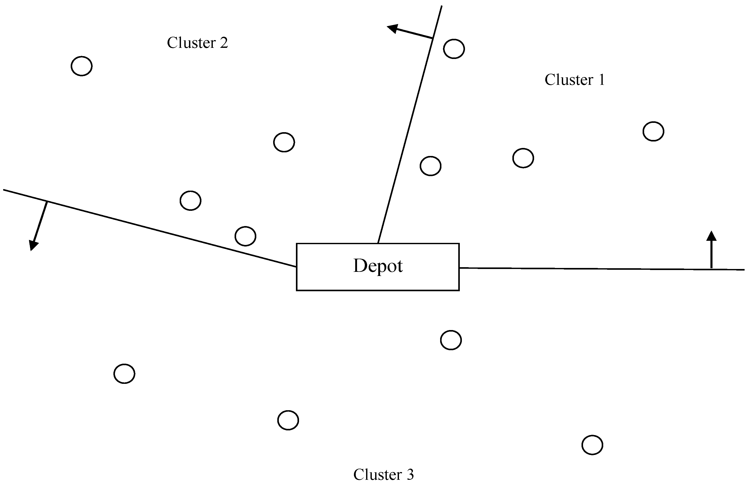
Hence, the first step of this stage was to convert the Cartesian coordinate system to the polar coordinate system and to use the depot as the origin. After that, sort the customers by their angle increasingly, and dispatch customers according to the order of the vehicles, until they cannot take another customer (the remaining customers were then dispatched to another empty vehicle). Repeat the procedure until all the customers have been dispatched to one vehicle. Figure 3 illustrates the forward sweep algorithm.

Figure 3.
Forward Sweep Algorithm.
2.2.2. Second Stage (k-Means Algorithm)
We obtained the initial k clusters of the customers after finishing the first stage of clustering, which means we could obtain the initial k centers of weight for the k-means algorithm by calculating the center of weight for each initial cluster. Before dispatching the customers via the k-means algorithm, we sort the customers by their demand decreasingly, since the customers with higher demands may cause more emission of CO2 and may have a larger influence on the objective function.
After sorting the dispatching order, we calculated the distances between the customer and k centers of weight; the clusters with the shorter distance had the higher priority for the customer to be dispatched to. Only the clusters with a remaining capacity that was not smaller than the demand of the customer would be candidates for the customer to be dispatched to. Then, the customer would be dispatched to the candidate cluster which had the highest priority among them. This procedure would be repeated until all the customers were already dispatched to one cluster. Then, we could update the centers of weight of the k clusters and repeat the customer dispatching until the centers of weight of the k clusters did not change anymore or reached the set number of iterations.
2.3. Genetic Algorithm with Quantum Random Number Generator Optimization
The first optimization method, after the clustering method, is the GAQ. The traditional GA have been long used to solve truck dispatching problems as the attributes used such as genes, chromosomes, and population are largely similar to sequence-related problems (or scheduling problems). For the design in this research, the genes in chromosomes were set to integer values, in order to simplify the process of conversion. We use the notations 1, 2, …, n to represent customers, and the sequence was the order for truck operators to visit customers. For example, a gene 5, 4, 3, 2, 1 meant that the truck operator will start from the depot to visit customer number 5, following customer number 4, and so on. The truck would be back to the depot after visiting customer number 1. The objective function of the GAQ was to search for an order of sequence that provided the minimum CO2 emission for delivery. While the GA was in iteration, the algorithms conduct several stages of operation including initialization, evaluation, selection, crossover and mutation until the final iteration was reached. In addition, all random numbers utilized in the GAQ in this research were generated by the QRNG (Section 2.3.6).
2.3.1. Initialization
In the initialization stage, we inserted the sequence that was the result from the clustering process; thus, the sequence length of each cluster is known. Then the population size was set up as 100. We randomized the initial sequences several times to serve and become the initial population.
2.3.2. Evaluation
After having the populations, we evaluated each of the populations through its fitness value. The fitness value comes from the accumulation of the CO2 emission calculation from beginning to the end of the population.
2.3.3. Selection
In the selection process, we used a modified roulette wheel method. We created a poll table based on the fitness value of the population. The poll table worked by having the fitness value of the population as fi = 1, 2, …, population size, and the accumulation of all the reciprocal of fitness value as . The probability of being selected was (1/fi)/F. However, if Max(fi) − Min(fi) << fi, the probability of selection would become more uniform, which means that the better choice would not receive a much higher probability to be selected and may cause the inefficiency of the model convergence.
Therefore, we introduced a new fitness value for the selection, as si = fi − Min(fi) × r, where r was a constant that 0 ≤ r < 1. The accumulation was , and the new probability of the selection was (1/si)/S. The bigger that r was set, the higher the probability of selecting relatively better chromosomes would be. In this research, we set the value of r to 0.9.
We generated a random number from zero to one. The number decided which population was selected to be the first parent, based on the poll table. To avoid selecting the same population to be the second parent, the poll table for the second parent was regenerated with the population without the first parent. Then, we generated another random number to decide which population was the second parent based on the new poll table.
2.3.4. Crossover
In the crossover stage, we generated a random value from zero to one and compared the number with the crossover probability. In the case that the random number was below or equal to the crossover probability, we would conduct a crossover to the previously selected two parents to produce two offspring. We inserted a roulette wheel to decide which crossover method was applied among partially mapped crossover, order one crossover, cycle crossover, and modified order crossover. The roulette wheel was created based on the fitness values of the parents applying each method.
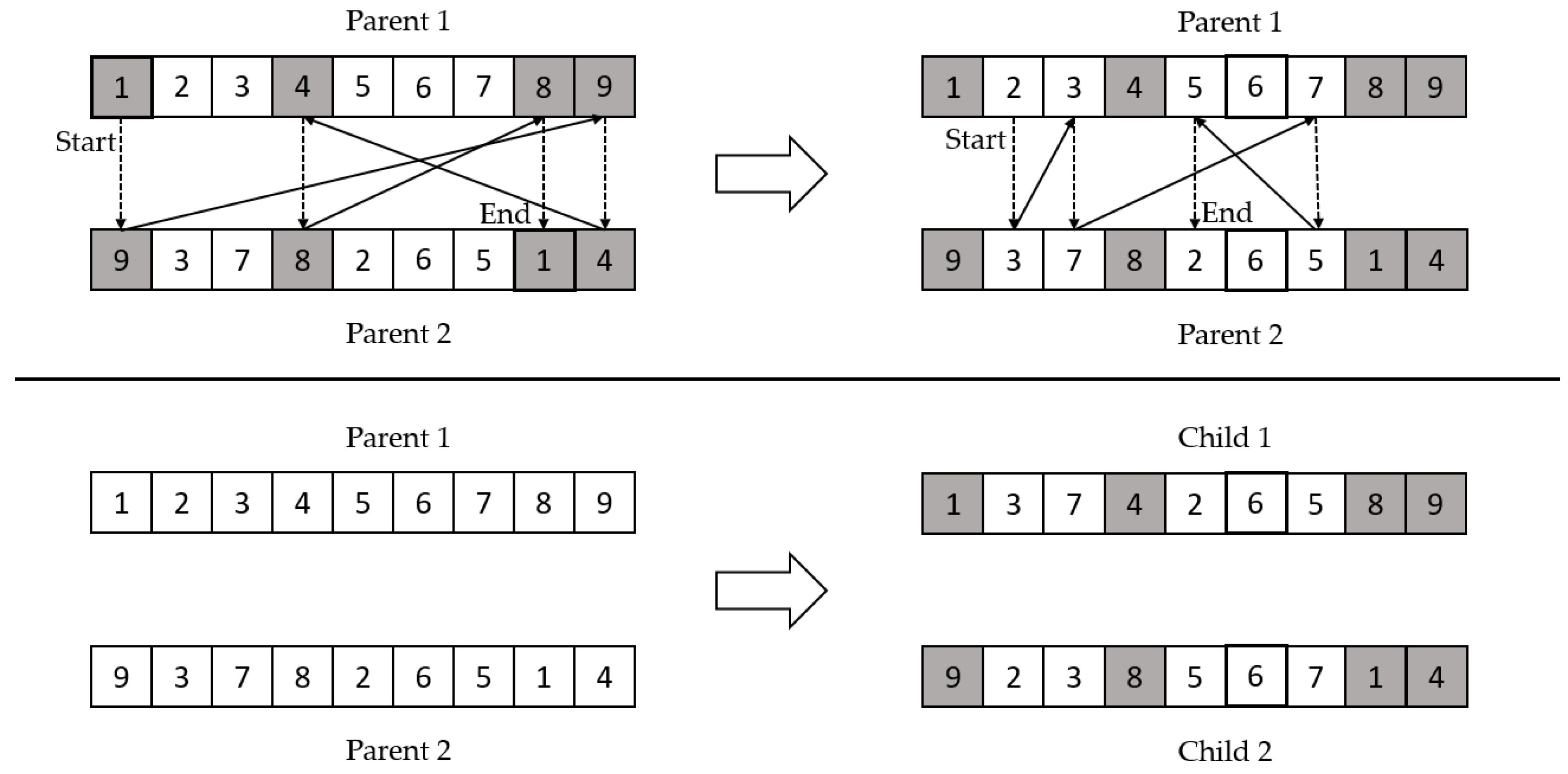
Partially mapped crossover generated offspring by choosing a sequence of elements from one parent and preserving the order and position of as many elements as possible from the other parent. It worked by having the child keep a section of the first and second parents, accordingly, and then recorded the elements in the gene number of the opposing parent those that were not in the child. Then, a mapped operation occurred, until the children were both completed. Figure 4 illustrated a partially mapped crossover example.
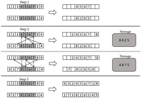
Figure 4.
Partially mapped crossover example.
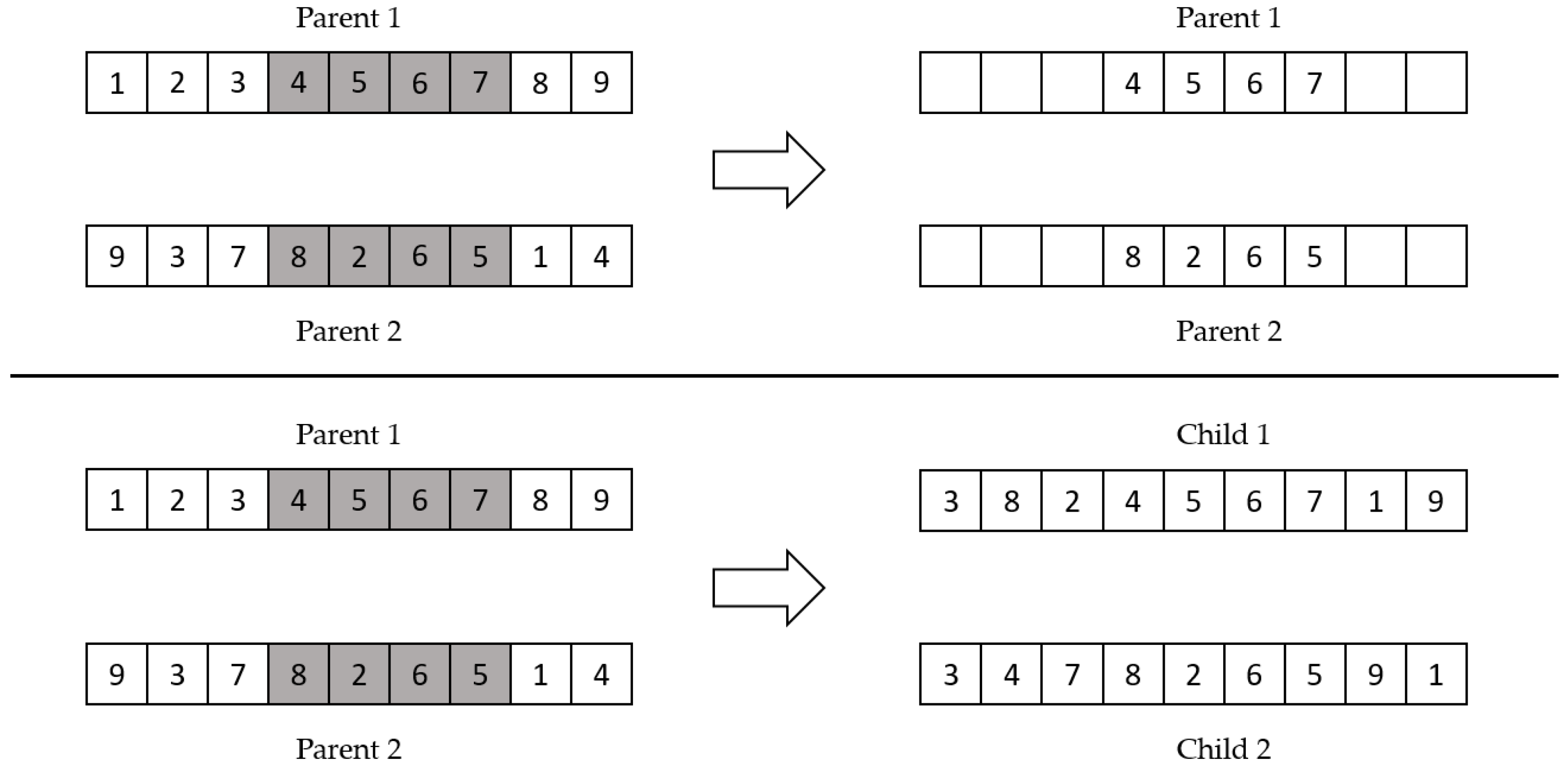
Order one crossover worked by selecting a section of the first parent to be set to the same gene number as the first child; the same goes for the second child. From there, we evaluated the next gene number based on the other parent; for the genes that were not yet in the child, we inserted the genes in ascending order, after the last genes in the section. Figure 5 simply illustrates the order one crossover example.
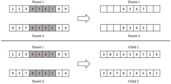
Figure 5.
Order one crossover example.
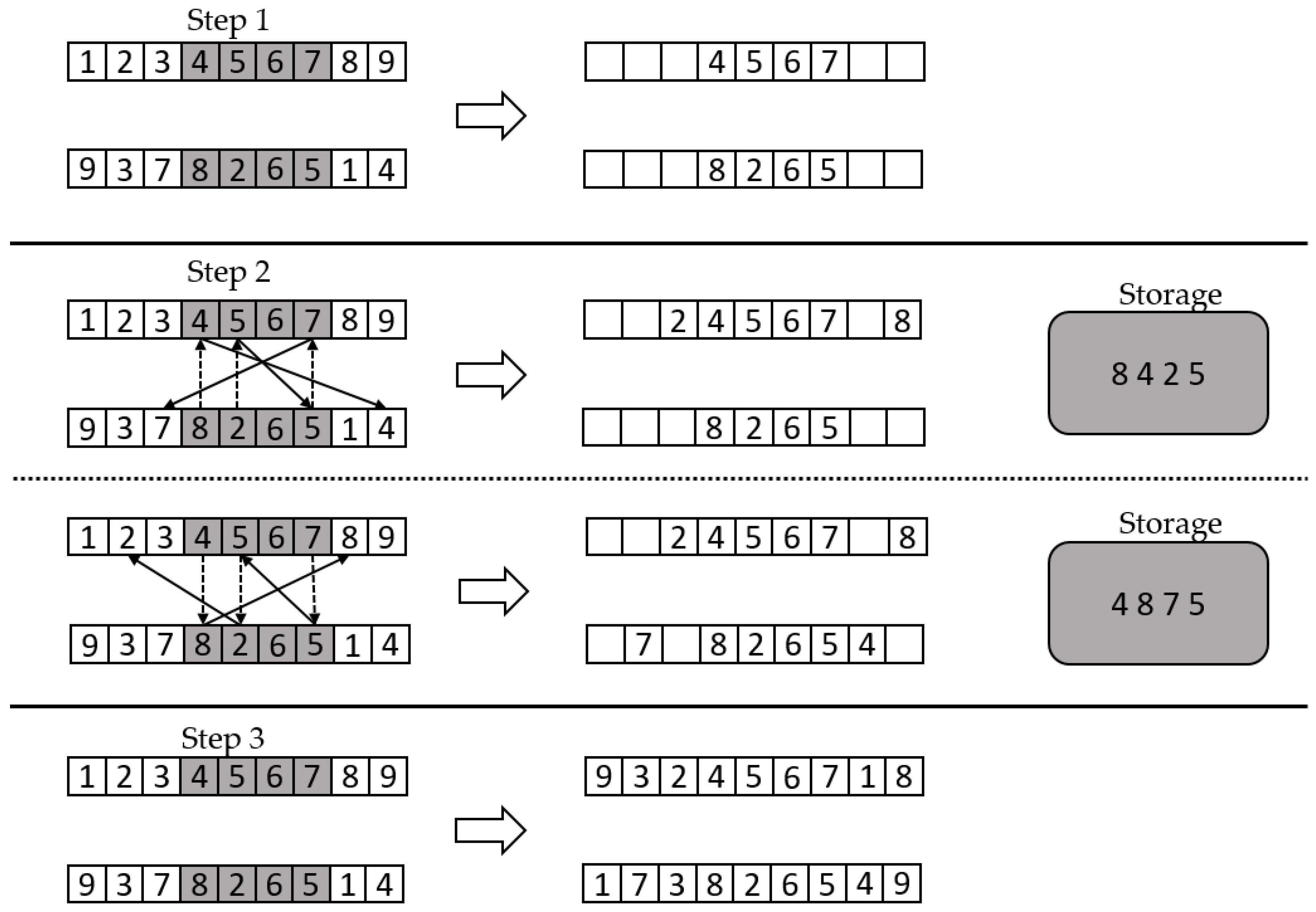
Cycle crossover worked by creating cycles between the two parents, such that the first element in parent one was matched with the first element in parent two. Next, we continued to find the elements from each other and inserted the elements in child one and child two, accordingly. Figure 6 shows an example of cycle crossover.
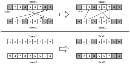
Figure 6.
Cycle crossover example.
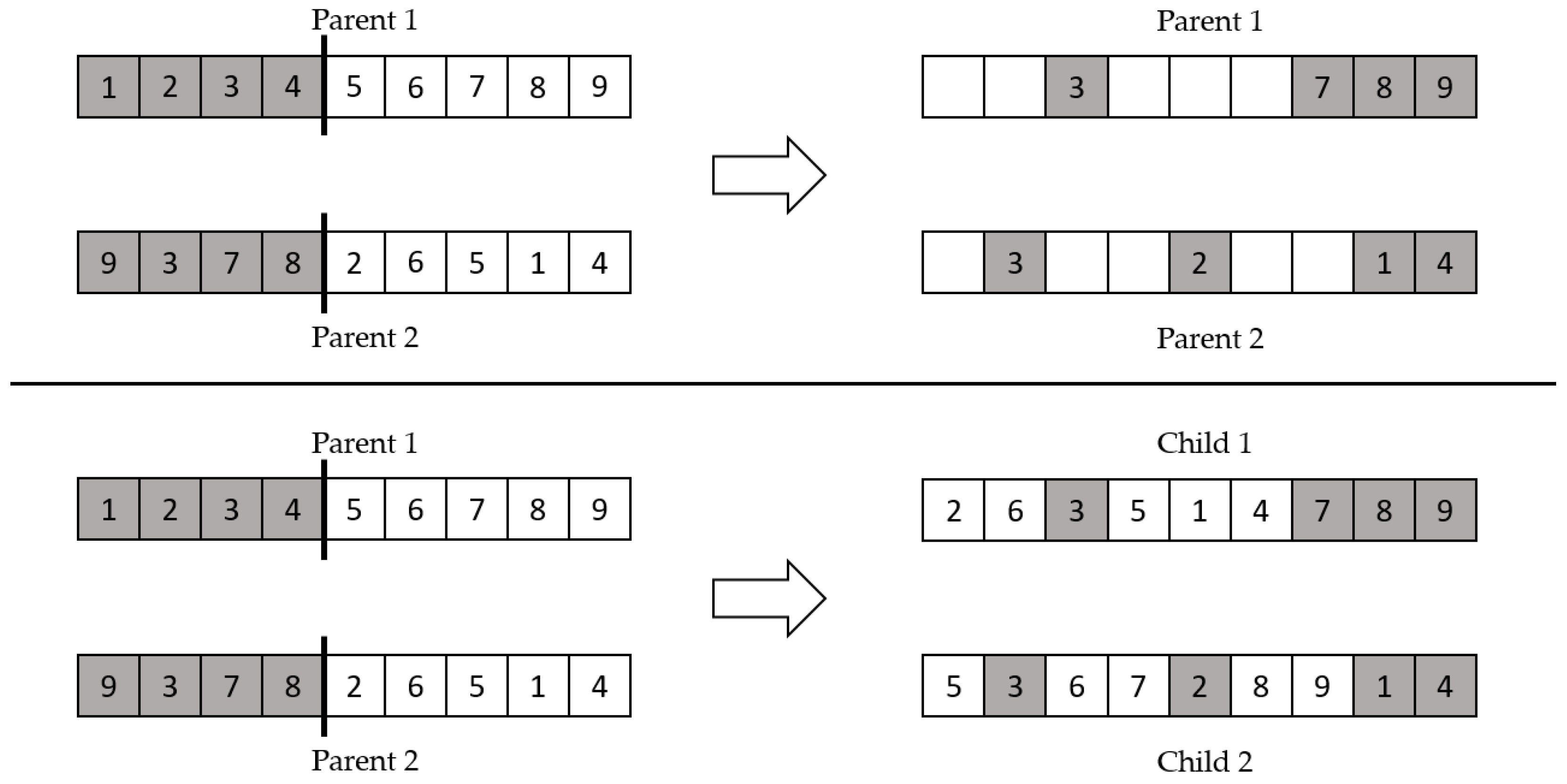
Modified order crossover divides the parents into right and left sections, at a randomly chosen crossover points. The right sections of the two parents were selected to be the preserving elements for the opposing parent and we got the children from the parents. Then, we inserted the left sections of the two parents to the empty parts of the child from the opposing parent, in order from left to right. Figure 7 illustrates an example of modified order crossover.
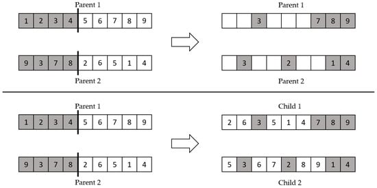
Figure 7.
Modified order crossover example.
2.3.5. Mutation
In the mutation stage, we generated a random number from zero to one and compared the number with the mutation probability. In the case that the random number was below or equal to the crossover probability, then we could conduct mutation to the previously produced offspring to produce a single offspring.
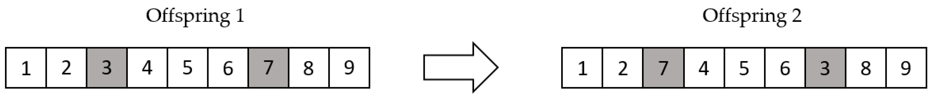
In this research, we applied two-point exchange methods to replace the traditional mutation method and completed the mutation process. We generated two positions of the offspring randomly, then exchanged the elements at these positions and produced the mutated offspring. The following Figure 8 illustrates a two-point exchange mutation example.
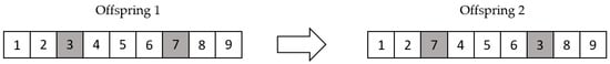
Figure 8.
Two-point exchange mutation example.
The generation in the GAQ, iterated while executing the mentioned stages (and executing the crossover and mutation) when the criteria was satisfied, until the last iteration was reached and had the best fitness value, in this case the minimum value.
2.3.6. ANU QRNG
In this research, all the randomness in the GAQ (such as random numbers that decided whether to execute crossover or mutation, random numbers that were used in roulette wheels, and random positions of crossover/mutation points) were acquired from the Australian National University QRNG server. We used the R package, called “qrng”, to retrieve quantum random numbers in real-time from the quantum computing server and integrated them into the GAQ coding. QRNG can provide true random numbers because of the inherent randomness at the core of quantum mechanics, which makes quantum systems a perfect source of entropy. Moreover, the difference between QRNG and PRNG is that QRNG has some unpredictable physical meanings to the generated numbers, and PRNG uses completely computer-generated probability distribution.
2.4. Tabu Search Optimization
The TS algorithm is a local search meta-heuristic and this method solves optimization problem widely. The TS guides a local heuristic search procedure to explore the solution space beyond local optimality. The TS is similar to the neighborhood search; that is, the TS begins in the same way as an ordinary neighborhood search, moving iteratively from one solution to another, until a solution is obtained. The motivation to construct the TS is that if one point has been visited once, there is no need to waste computation time to revisit and reevaluate that point.
Contrary to classical methods, the current solution generated from the TS may worsen from one iteration to the next. Thus, solutions possessing some attributes of recently explorations are temporarily declared Tabu or forbidden, unless their cost is less than a so-called aspiration level, to avoid cycling. The aspiration level is a condition that can override the Tabu restraint, if the question is minimizing the problem and movement is Tabu, but objective value is smaller than aspiration level, we allow the movement at this time. A move is defined as going from one solution to another. Moreover, the TS method has some parameters, which need to be set before calculation. It contains a Tabu tenure, a candidate list, and an aspiration condition. The Tabu tenure is the length of time during which a certain move is classified as the Tabu. The candidate list contains all the nodes that can be swapped. Obviously, the size of the TS’s candidate list is an important factor. The author of [28] suggested that the ideal candidate size is between n and 2n. In general, there are two types of memory in the TS: recency-based memory and frequency-based memory, characteristics are as follows in Table 1:

Table 1.
Comparison of recency-based memory and frequency-based memory.
In this research, the TS method used the recency-based memory to avoid the reversal of moves and cycling. The following Table 2 was our TS’s process.
Table 2.
The steps of the TS Algorithm.
2.5. Two Hybrid Models for Minimizing CO2
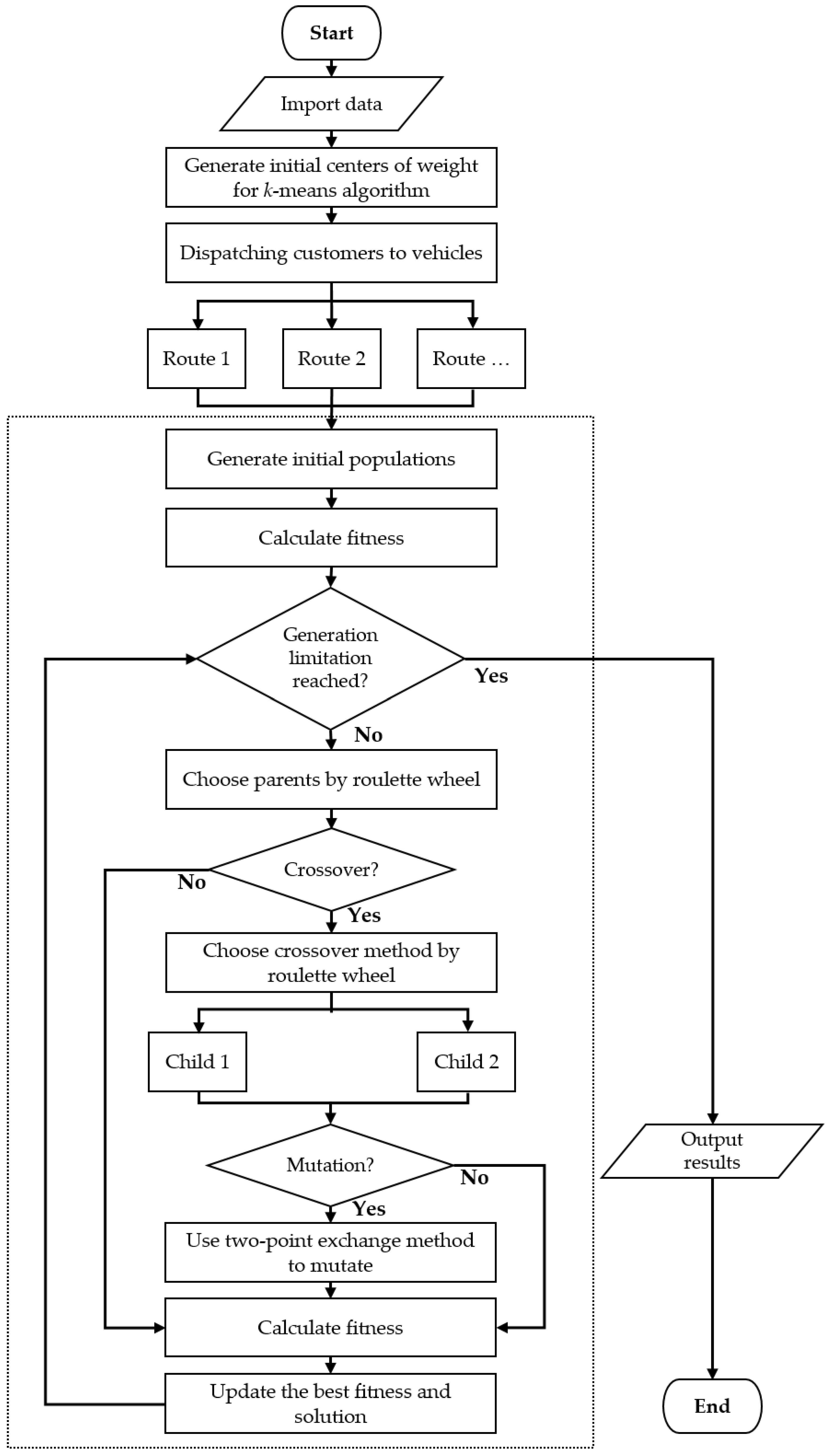
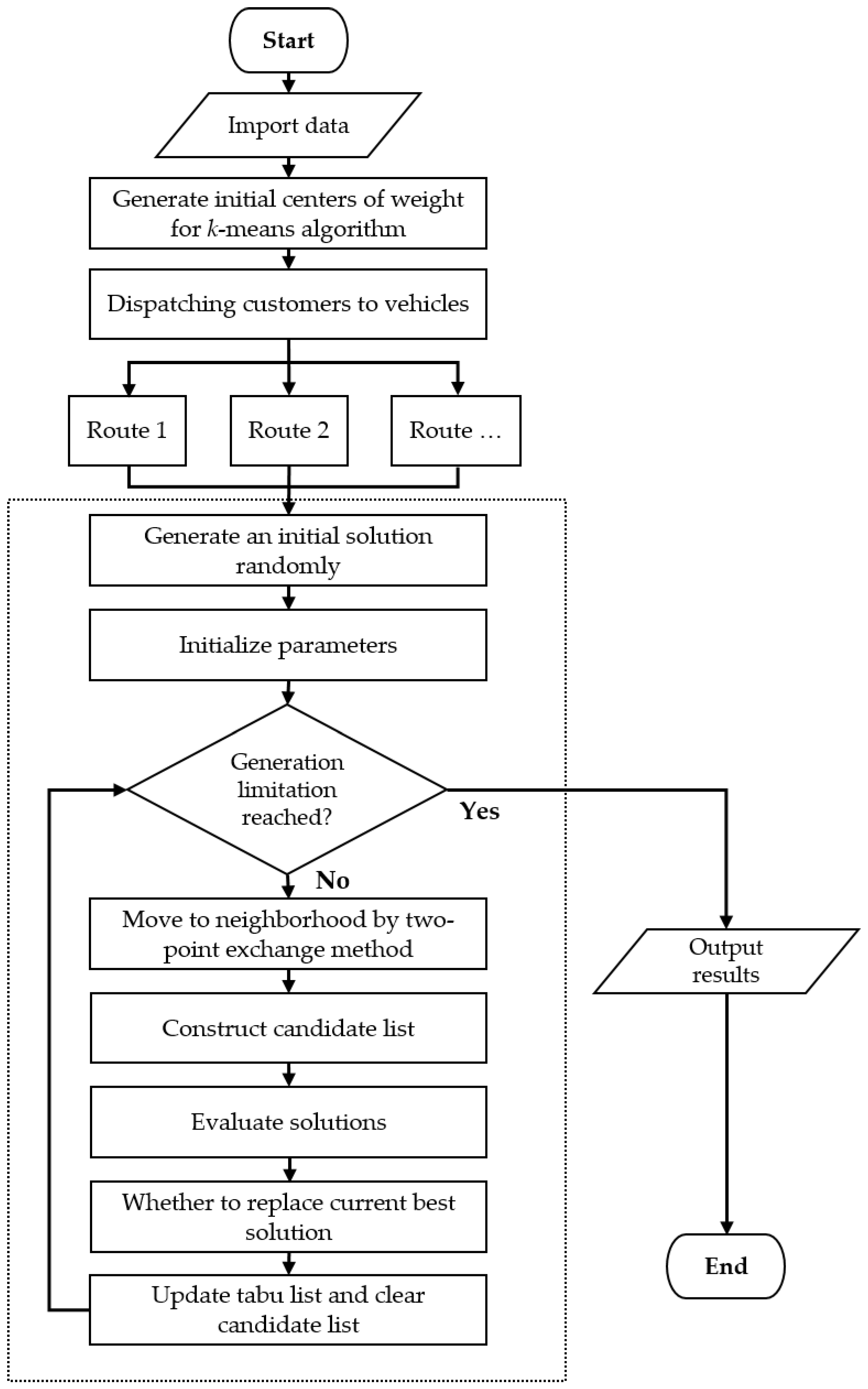
In this research, we proposed two hybrid models to solve the PRPs. In the beginning, we used a two-stage method combining the sweep algorithm and the k-means algorithm for dispatching customers to k vehicles. After completing clustering, the PRP was divided into several TSPs. Finally, we used the GAQ and the TS to optimize every route from the grouping results in the first phase. Combing the above step, the second phase optimization, via the GAQ, was our first hybrid model, called k-means clustering with genetic algorithm with QRNG (kGAQ) and k-means clustering with tabu search optimization was the second hybrid model (kTS). The pseudo-code (Table 3 and Table 4) and procedures (Figure 9 and Figure 10) of the two hybrid models are shown as follows.
Table 3.
The pseudo-code of kGAQ.
Table 4.
The pseudo-code of kTS.
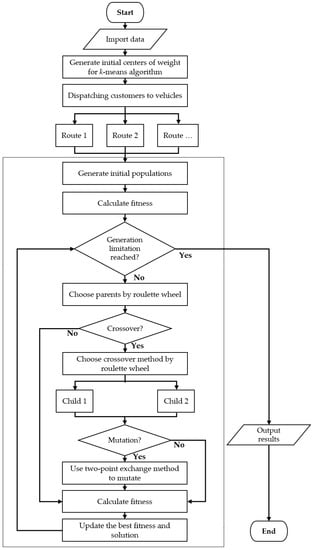
Figure 9.
The procedure of kGAQ model.
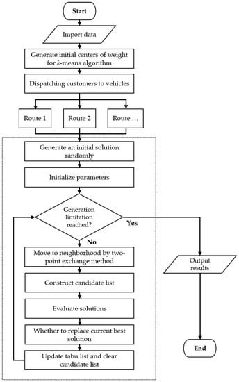
Figure 10.
The procedure of kTS Model.
3. Computational Results
In this section, we discuss the results of the computational experiments from the two hybrid models, based on their performance on the benchmark problems. We selected 30 benchmark problems to experiment from set A and set B (proposed by the authors of [29]) and set E (proposed by the authors of [30]). The objective of the experiment in this study was to minimize the emission of CO2 during the delivery. The parameters for the adjustment of the kGAQ and the kTS were determined through the Design of Experiments.
The settings of the kGAQ were as follows:
- Iteration per run was 10,000.
- Population was 100.
- Crossover probability was 0.95.
- Mutation probability was 0.025.
The settings of the kTS were as follows:
- Iteration per run was 10,000.
- Tabu tenure was 6.
- Size of candidate list was 2n.
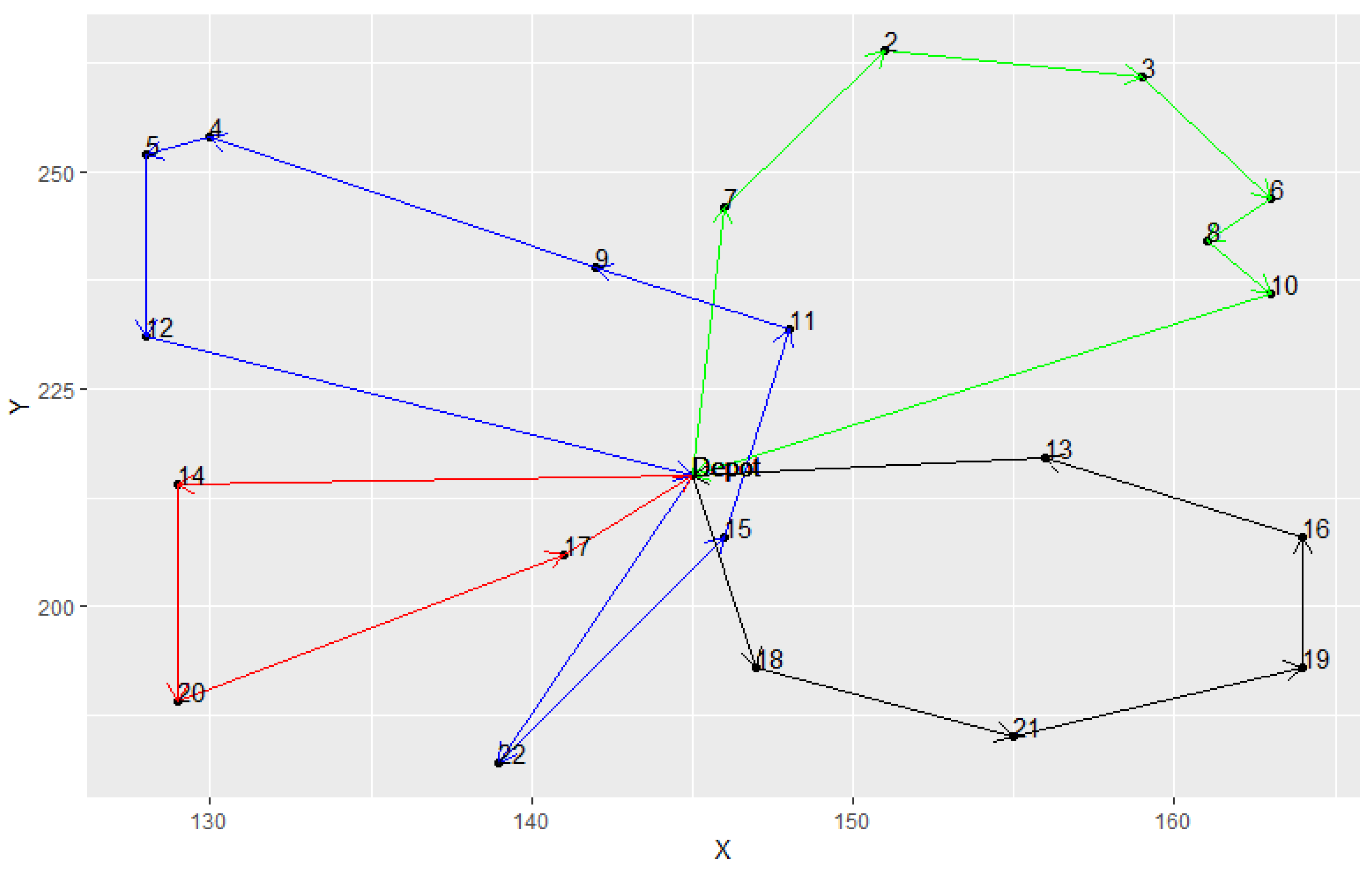
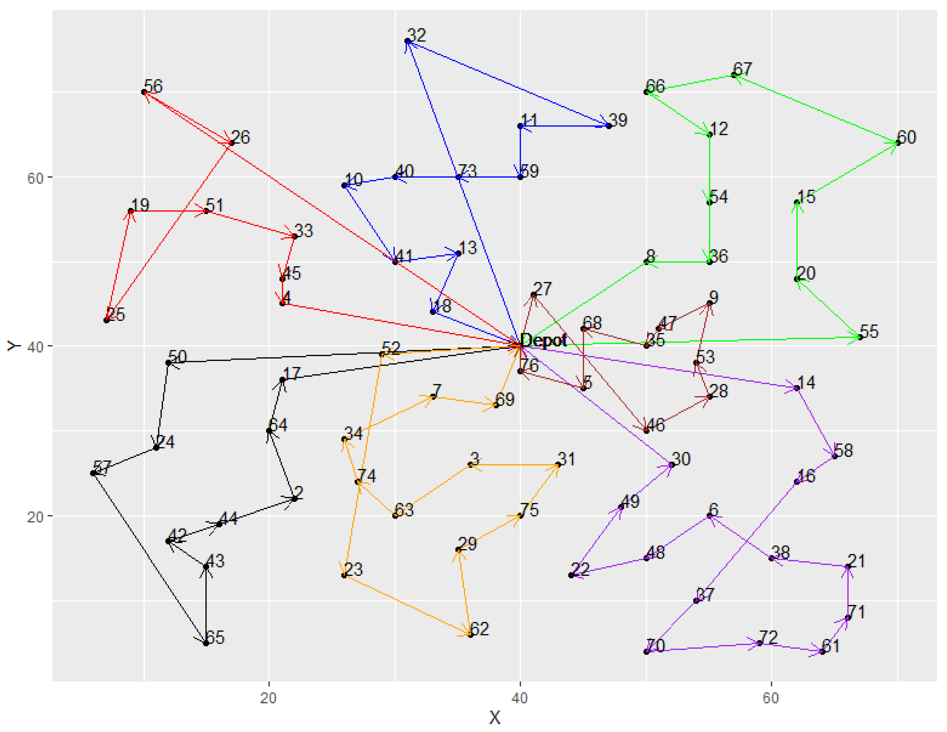
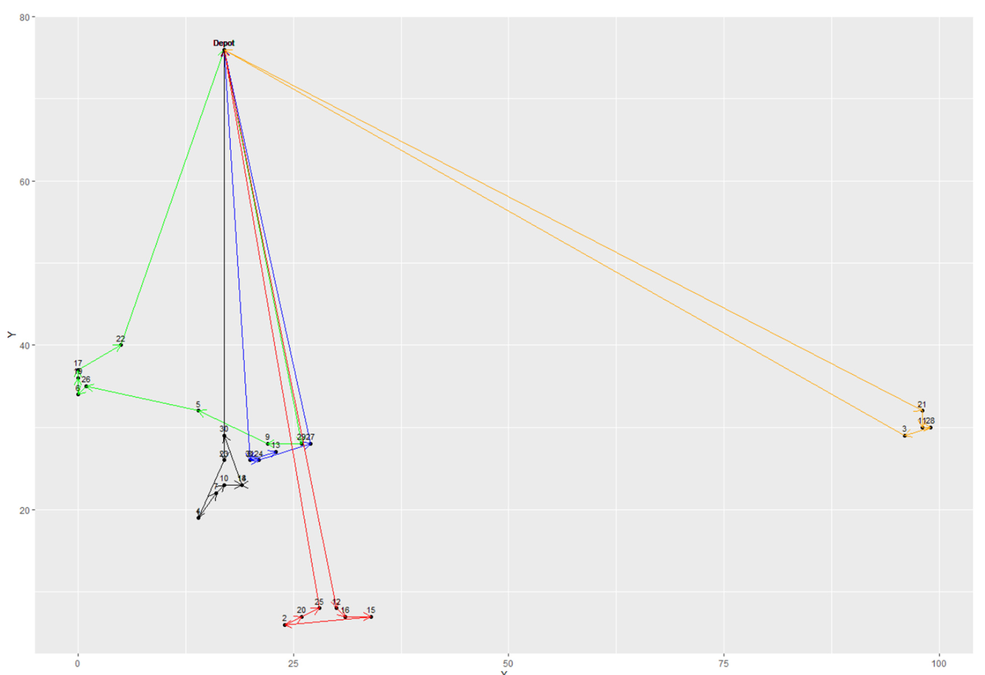
From Table 5, it was observed that both hybrid models provided good solution quality and had the same best results in most instances. However, the average results of the TS were all better than the kGAQ, except in instances A-n32-k5 and E-n101-k8. Meanwhile, the standard deviations of kTS were smaller than the kGAQ. In addition, Figure 11, Figure 12 and Figure 13 illustrated the best solutions for instances E-n22-k4, E-n76-k7, and B-n31-k5, respectively, provided by the kGAQ. We found that the kGAQ can produce a fair solution quality for both small-scale and large-scale problems. From the routing graph, we found that the results sometimes had cross-roads that normally should not occur in traditional TSPs because the emission of CO2 is not only related to the travel distance but also the weight of vehicles. That is, customers with large amounts of demands may have lower priority to be visited, according to the properties of the PRPs. Figure 13 shows that kGAQ can provide fair results when the location of the depot is not in the center of the map.
Table 5.
The experimental results of the two hybrid models with different optimization methods. (CO2 Unit: Kg).
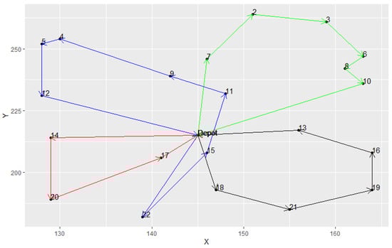
Figure 11.
The best solution provided by kGAQ in instance E-n22-k4.
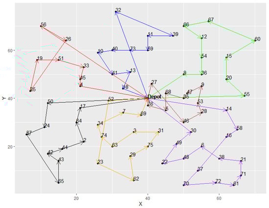
Figure 12.
The best solution provided by kGAQ in instance E-n76-k7.
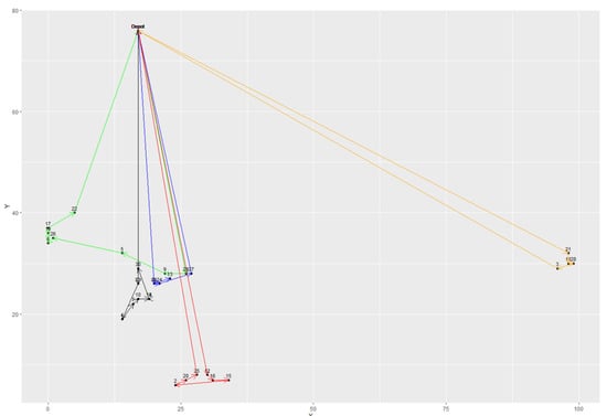
Figure 13.
The best solution provided by kGAQ in instance B-n31-k5.
4. Conclusions
In this research, we applied a two-stage clustering method to assign customers to trucks based on their demands, combining with the sweep algorithm and the k-means algorithm in the first phase as clustering first approach. We then used the GAQ and TS to minimize the CO2 emission along every route in the second phase (for our proposed hybrid models). The major contribution in this paper is that the traditional GA has only one crossover method and one mutation method to produce offspring, which means that each individual could only search for solutions in one dimension for each iteration. In our design, we developed a new crossover process and a new mutation process for the purposed model, including four different crossover methods and four different mutation methods, to realize finite quantum search dimension. The selection process was achieved through a quantum random number generator, which was optimized to reduce the offspring’s fitness value, produced by each method in the proposed hybrid model.
The results from the experiment proved that both hybrid models could provide good solutions, with fair quality for CO2 emission minimization for 29 PRPs out of a total of 30 instances (30 runs each for all problems) and showed no difference between the best results on each instance, if not the same. This research is applicable and usable for solving real-world problems from various fields, especially in sustainable logistics management. Solving the PRPs to minimize carbon dioxide emission reduces fuel consumption and lowers the environmental impacts, following one of the seventeen sustainable development goals set by the United Nations.
For further research, modern metaheuristic algorithms may be considered to increase calculation performance. More advanced quantum computing technology may be applied when quantum computers are widely used in the world.
Author Contributions
Conceptualization, S.-C.L. and Y.-C.S.; methodology, S.-C.L. and Y.-C.S.; validation, S.-C.L. and Y.-C.S.; formal analysis, S.-C.L. and Y.-C.S.; experiment, S.-C.L. and Y.-C.S.; writing—original draft preparation, S.-C.L. and Y.-C.S.; writing—review and editing, S.-C.L. and Y.-C.S.; visualization, S.-C.L. and Y.-C.S.; supervision, S.-C.L. and Y.-C.S.; funding acquisition, S.-C.L. Both authors have read and agreed to the published version of the manuscript.
Funding
This research was funded by the Ministry of Science and Technology, Taiwan, grant number 109-2637-H-011-002.
Institutional Review Board Statement
Not applicable.
Informed Consent Statement
Not applicable.
Acknowledgments
The authors would like to thank the editors and reviewers for their professional and valuable comments and suggestions that helped improve the quality and value of this study.
Conflicts of Interest
The authors declare no conflict of interest.
References
- Kanniah, K.D.; Zaman, N.A.F.K.; Kaskaoutis, D.G.; Latif, M.T. COVID-19’s impact on the atmospheric environment in the Southeast Asia region. Sci. Total Environ. 2020, 736, 139658. [Google Scholar] [CrossRef]
- Maxie, E. Supplier performance and the environment. In Proceedings of the 1994 IEEE International Symposium on Electronics and The Environment, San Francisco, CA, USA, 2–4 May 1994; pp. 323–327. [Google Scholar] [CrossRef]
- Dantzig, G.B.; Ramser, J.H. The truck dispatching problem. Manag. Sci. 1959, 6, 80–91. [Google Scholar] [CrossRef]
- Gillett, B.E.; Miller, L.R. A heuristic algorithm for the vehicle-dispatch problem. Oper. Res. 1974, 22, 340–349. [Google Scholar] [CrossRef]
- Laporte, G. Fifty years of vehicle routing. Transp. Sci. 2009, 43, 408–416. [Google Scholar] [CrossRef]
- Yu, V.F.; Redi, A.A.N.R.; Hidayat, Y.A.; Wibowo, O.J. A simulated annealing heuristic for the hybrid vehicle routing problem. Appl. Soft Comput. 2017, 53, 119–132. [Google Scholar] [CrossRef]
- Bektaş, T.; Laporte, G. The pollution-routing problem. Transp. Res. B Meth. 2011, 45, 1232–1250. [Google Scholar] [CrossRef]
- Demira, E.; Bektaş, T.; Laporte, G. The bi-objective pollution-routing problem. Eur. J. Oper. Res. 2014, 232, 464–478. [Google Scholar] [CrossRef]
- Franceschetti, A.; Demir, E.; Honhon, D.; Van Woensel, T.; Laporte, G.; Stobbe, M. A metaheuristic for the time-dependent pollution-routing problem. Eur. J. Oper. Res. 2017, 259, 972–991. [Google Scholar] [CrossRef] [Green Version]
- Xiao, Y.; Zuo, X.; Huang, J.; Konak, A.; Xu, Y. The continuous pollution routing problem. Appl. Math. Comput. 2020, 387, 125072. [Google Scholar] [CrossRef]
- Erdoğan, S.; Miller-Hooks, E. A green vehicle routing problem. Transp. Res. E Log. 2012, 48, 100–114. [Google Scholar] [CrossRef]
- Dahi, Z.A.E.M.; Mezioud, C.; Draa, A. A quantum-inspired genetic algorithm for solving the antenna positioning problem. Swarm Evol. Comput. 2016, 31, 24–63. [Google Scholar] [CrossRef]
- Liu, R.; Jiang, Z. A hybrid large-neighborhood search algorithm for the cumulative capacitated vehicle routing problem with time-window constraints. Appl. Soft Comput. 2019, 80, 18–30. [Google Scholar] [CrossRef]
- Holland, J.H. Adaptation in Natural and Artificial Systems: An Introductory Analysis with Applications to Biology, Control, and Artificial Intelligence; University of Michigan Press: Ann Arbor, MI, USA, 1975. [Google Scholar]
- Haghani, A.; Jung, S. A dynamic vehicle routing problem with time-dependent travel times. Comput. Oper. Res. 2005, 32, 2959–2986. [Google Scholar] [CrossRef]
- Ghoseiri, K.; Ghannadpour, S.F. Multi-objective vehicle routing problem with time windows using goal programming and genetic algorithm. Appl. Soft Comput. 2010, 10, 1096–1107. [Google Scholar] [CrossRef]
- Xiao, Y.; Konak, A. A genetic algorithm with exact dynamic programming for the green vehicle routing & scheduling problem. J. Clean. Prod. 2017, 167, 1450–1463. [Google Scholar] [CrossRef]
- Glover, F. Future paths for integer programming and links to artificial intelligence. Comput. Oper. Res. 1986, 13, 533–549. [Google Scholar] [CrossRef]
- Glover, F. Tabu search: A tutorial. Interfaces (Providence) 1990, 20, 74–94. [Google Scholar] [CrossRef] [Green Version]
- Brandão, J.; Mercer, A. A tabu search algorithm for the multi-trip vehicle routing and scheduling problem. Eur. J. Oper. Res. 1997, 100, 180–191. [Google Scholar] [CrossRef]
- Barbarosoglu, G.; Ozgur, D. A tabu search algorithm for the vehicle routing problem. Comput. Oper. Res. 1999, 26, 255–270. [Google Scholar] [CrossRef]
- Du, L.; He, R. Combining nearest neighbor search with tabu search for large-scale vehicle routing problem. Phys. Procedia 2012, 25, 1536–1546. [Google Scholar] [CrossRef] [Green Version]
- Feynman, R.P. Simulating physics with computers. Int. J. Theor. Phys. 1982, 21, 467–488. [Google Scholar] [CrossRef]
- Herrero-Collantes, M.; Garcia-Escartin, J.C. Quantum random number generators. Rev. Mod. Phys. 2017, 89, 015004. [Google Scholar] [CrossRef] [Green Version]
- Jennewein, T.; Achleitner, U.; Weihs, G.; Weinfurter, H.; Zeilinger, A. A fast and compact quantum random number generator. Rev. Sci. Instrum. 2000, 71, 1675. [Google Scholar] [CrossRef] [Green Version]
- Stefanov, A.; Gisin, N.; Guinnard, O.; Guinnard, L.; Zbinden, H. Optical quantum random number generator. J. Mod. Opt. 2000, 47, 595–598. [Google Scholar] [CrossRef] [Green Version]
- Forgy, E.W. Cluster analysis of multivariate data: Efficiency versus interpretability of classifications. Biometrics 1965, 21, 768–769. [Google Scholar]
- Alander, J.T. On optimal population size of genetic algorithms. In Proceedings of the CompEuro 1992 Proceedings Computer Systems and Software Engineering, The Hague, The Netherlands, 4–8 May 1992; pp. 65–70. [Google Scholar] [CrossRef]
- Augerat, P.; Belenguer, J.M.; Benavent, E.; Corberan, A.; Naddef, D.; Rinaldi, G. Computational Results with a Branch and Cut Code for the Capacitated Vehicle Routing Problem; Institut National Polytechnique, 38: Grenoble, France, 1995. [Google Scholar]
- Christofides, N.; Eilon, S. An algorithm for the vehicle-dispatching problem. J. Oper. Res. Soc. 1969, 20, 309–318. [Google Scholar] [CrossRef]


Publisher’s Note: MDPI stays neutral with regard to jurisdictional claims in published maps and institutional affiliations. |
© 2021 by the authors. Licensee MDPI, Basel, Switzerland. This article is an open access article distributed under the terms and conditions of the Creative Commons Attribution (CC BY) license (https://creativecommons.org/licenses/by/4.0/).