
Effects of Water-Saving Irrigation on Hydrological Cycle in an Irrigation District of Northern China

Abstract
:1. Introduction
2. Methods
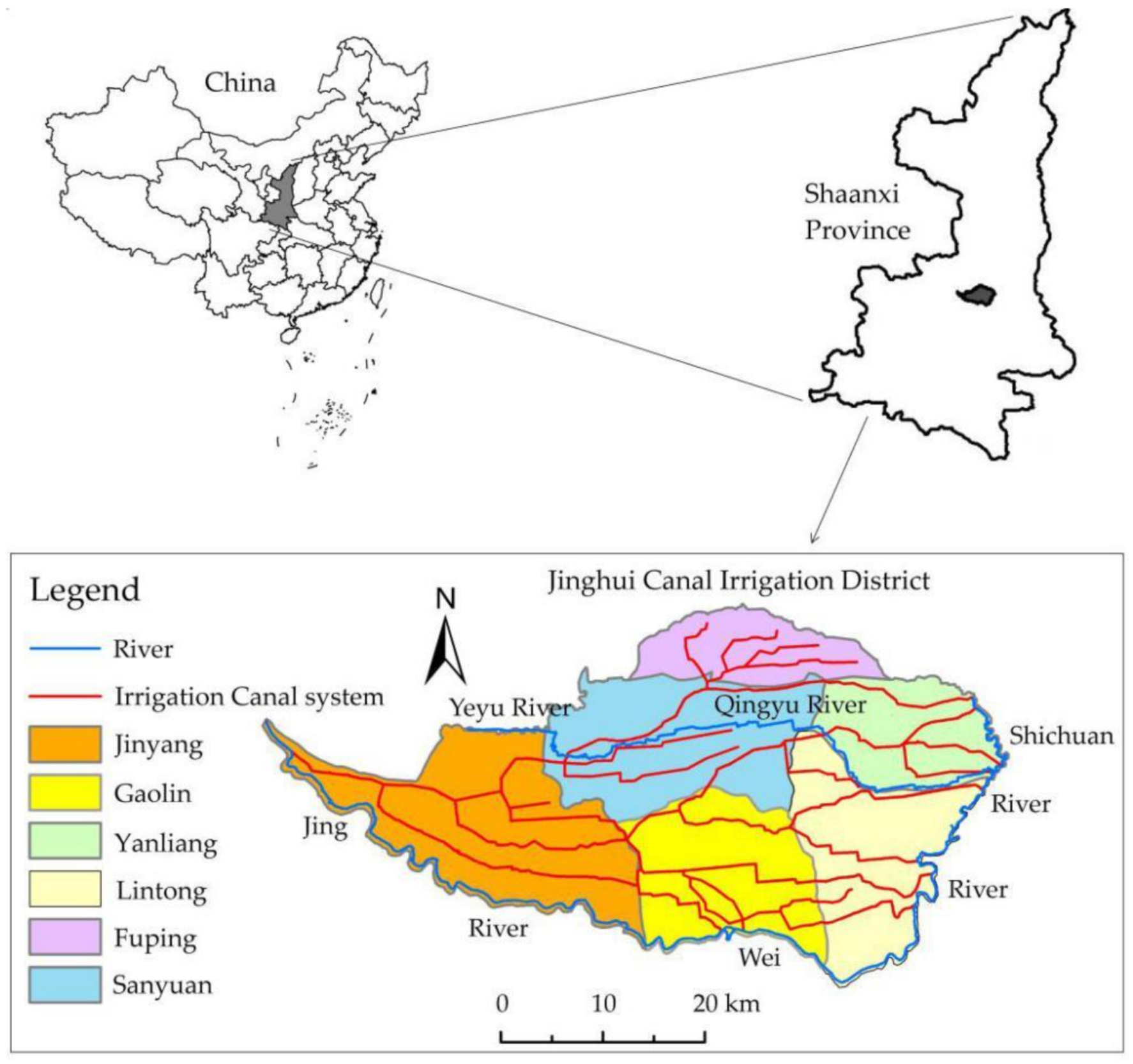
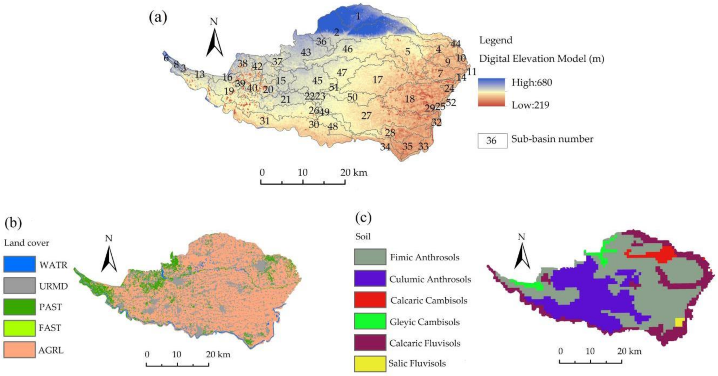
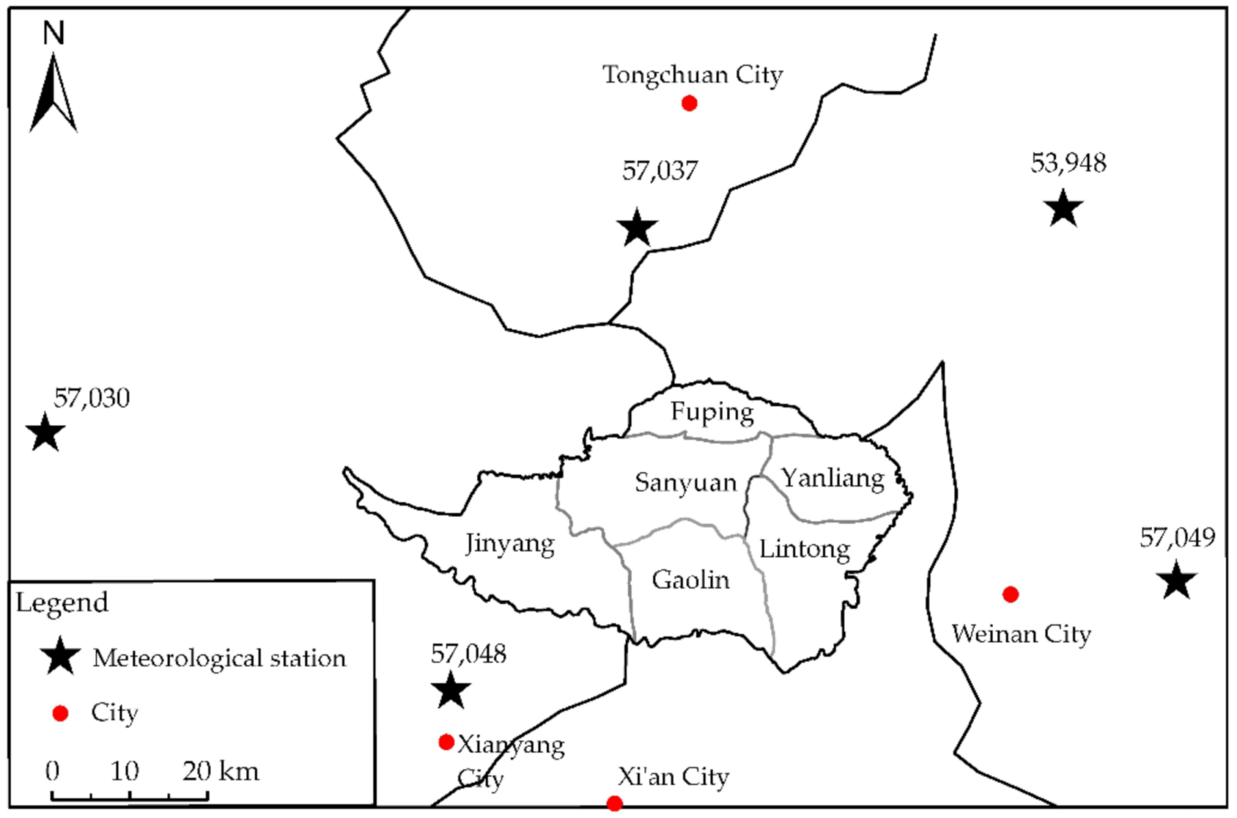
2.1. Study Area
2.2. Soil and Water Assessment Tool
2.3. Input Datasets
2.3.1. Physiographical Maps
2.3.2. Meteorological Data
2.3.3. Irrigation Data
2.3.4. Model Setup
2.3.5. Model Calibration
3. Results and Discussion
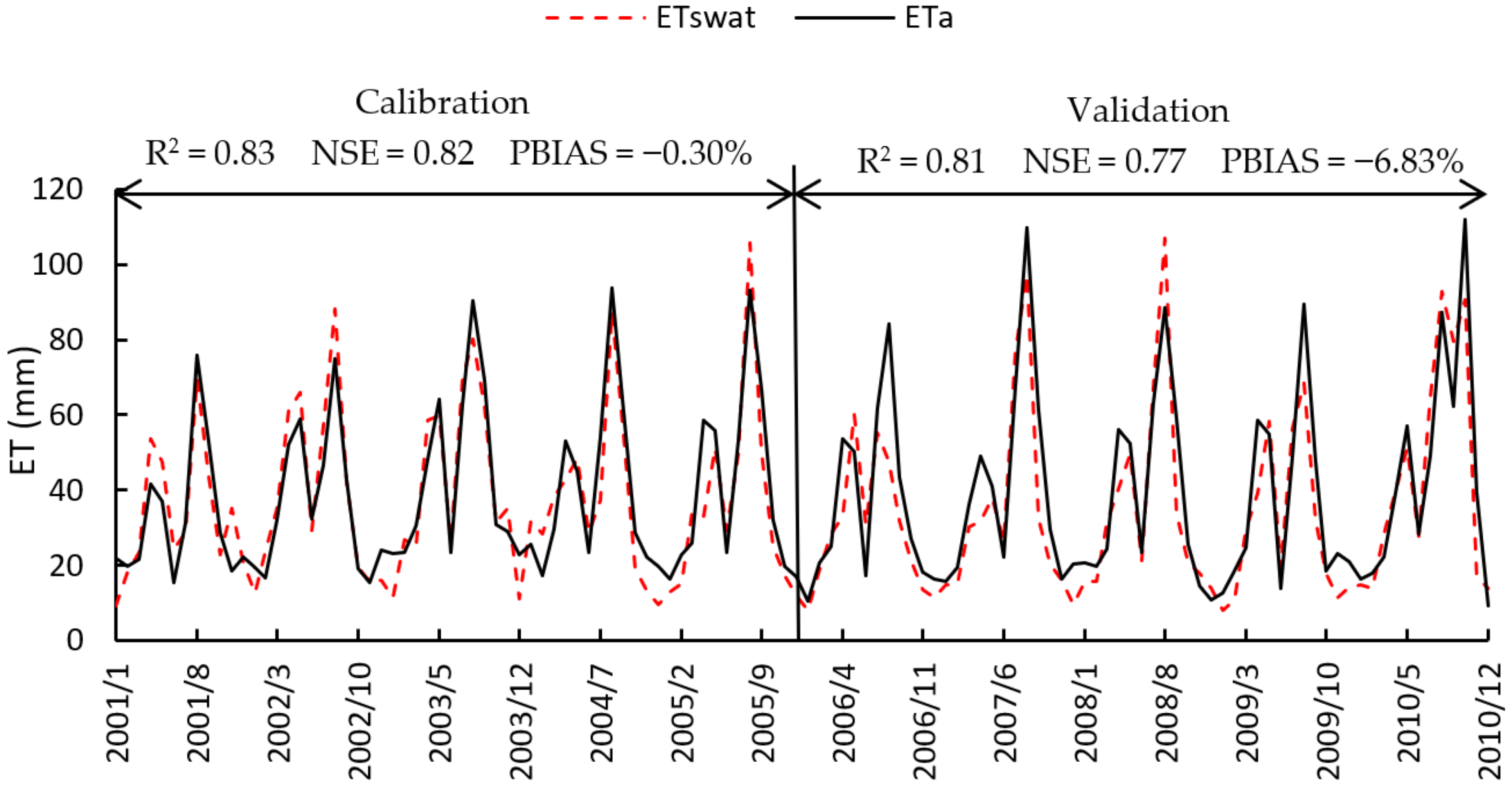
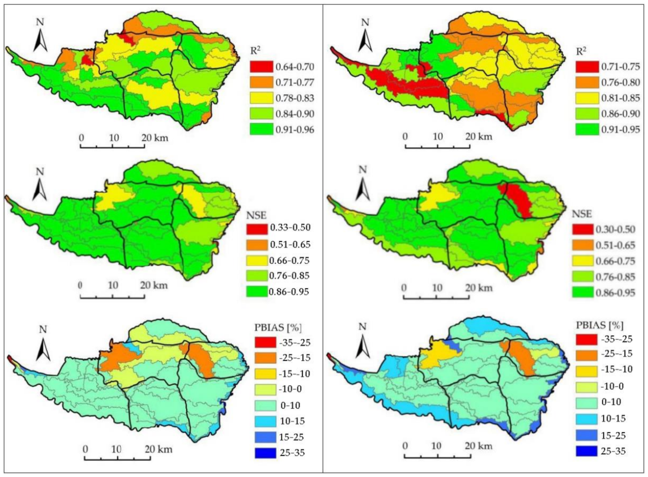
3.1. Calibration and Validation Results
3.2. Impacts of Water-Saving Irrigation on Hydrological Cycle Components
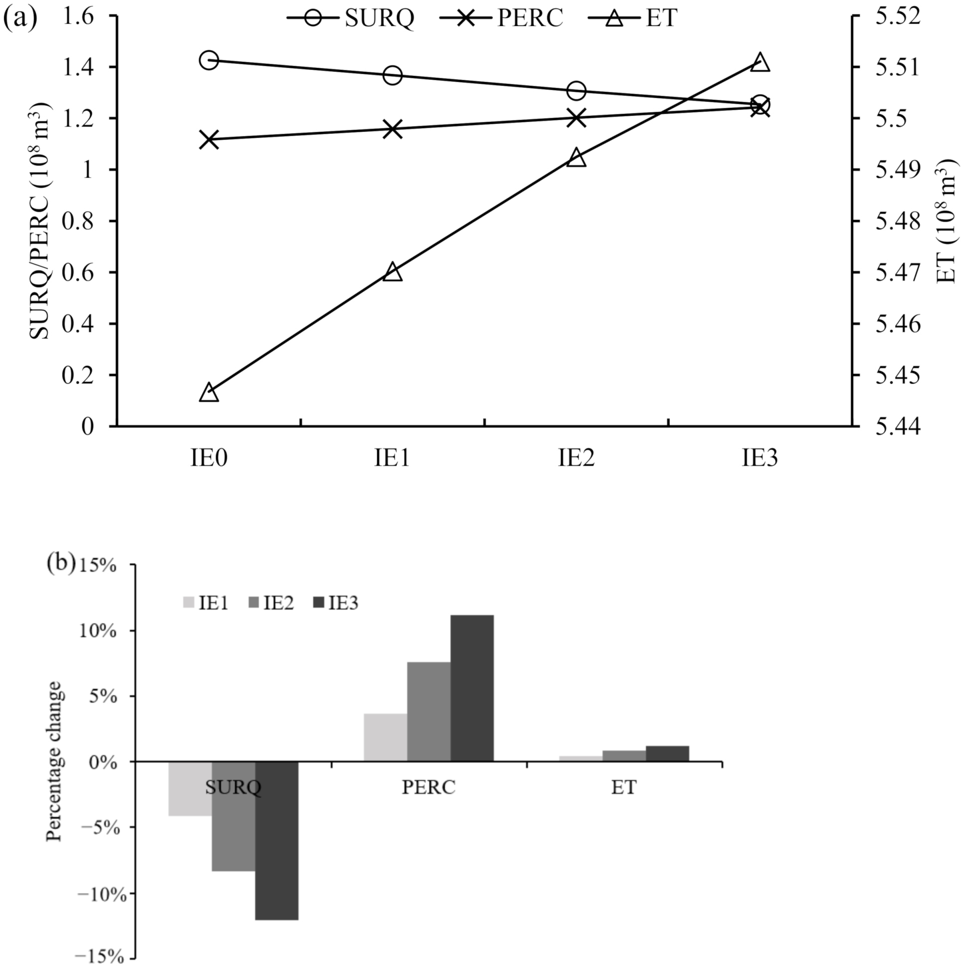
3.2.1. Annual Average Scale
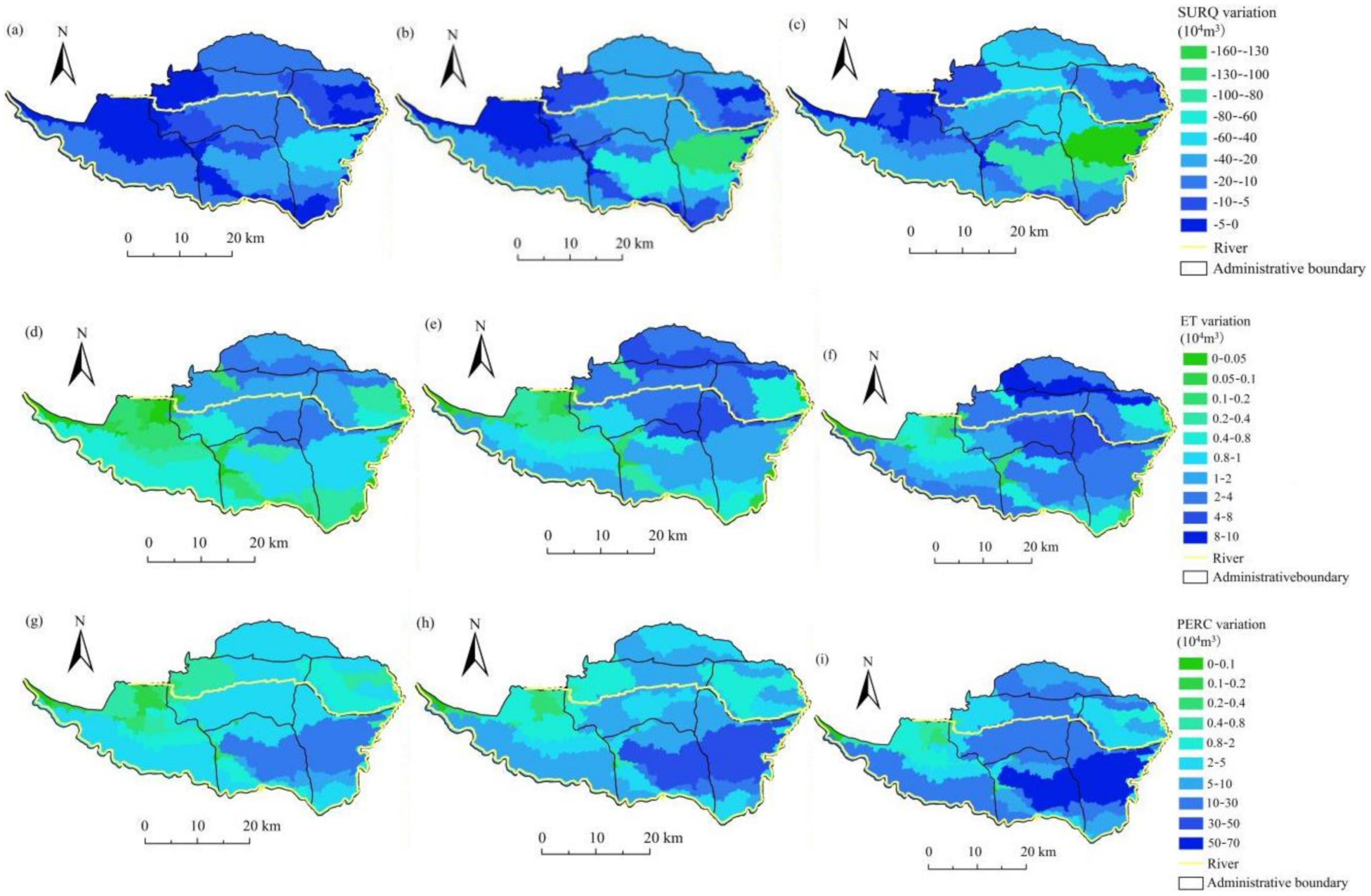
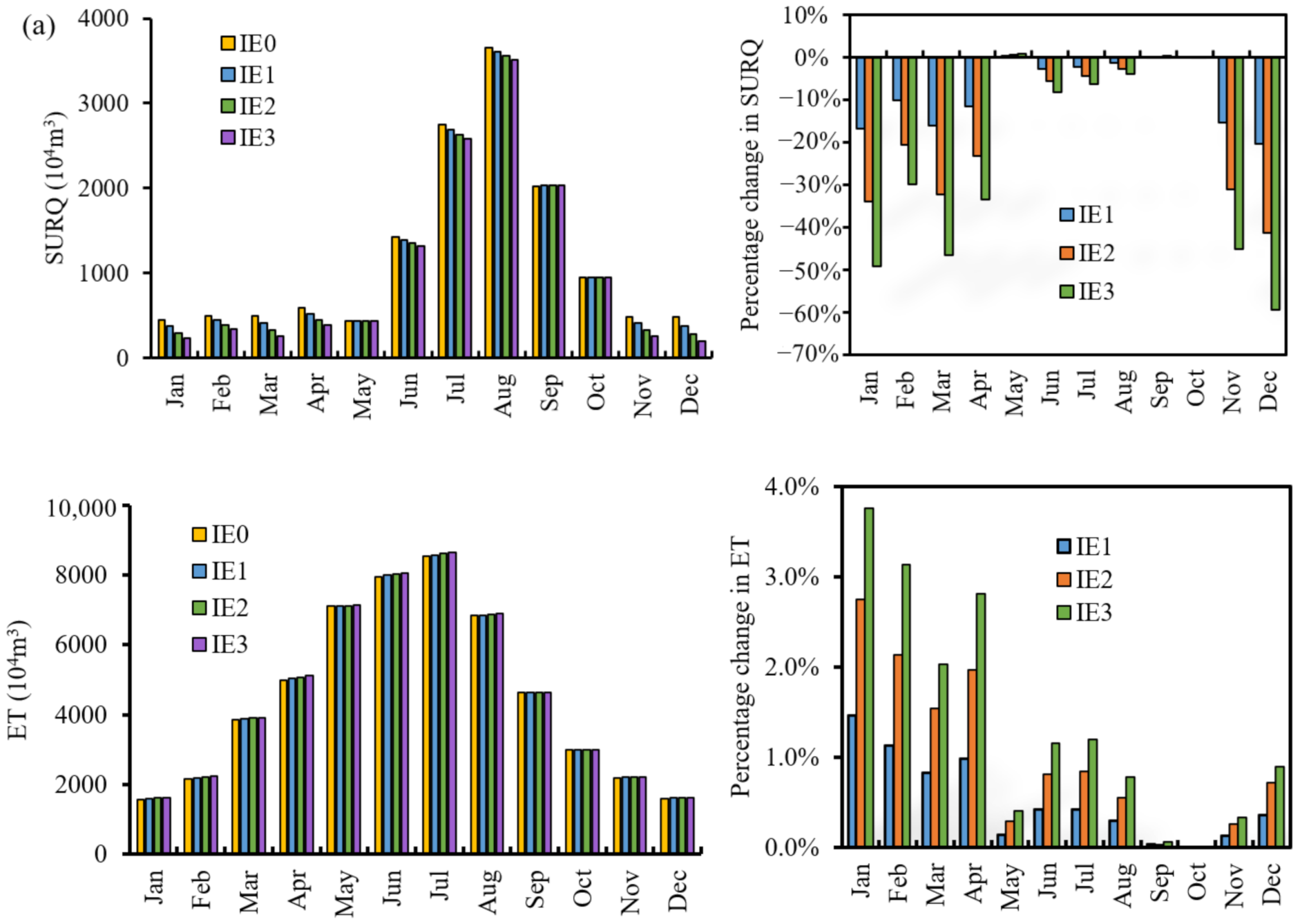
3.2.2. Monthly Average Scale
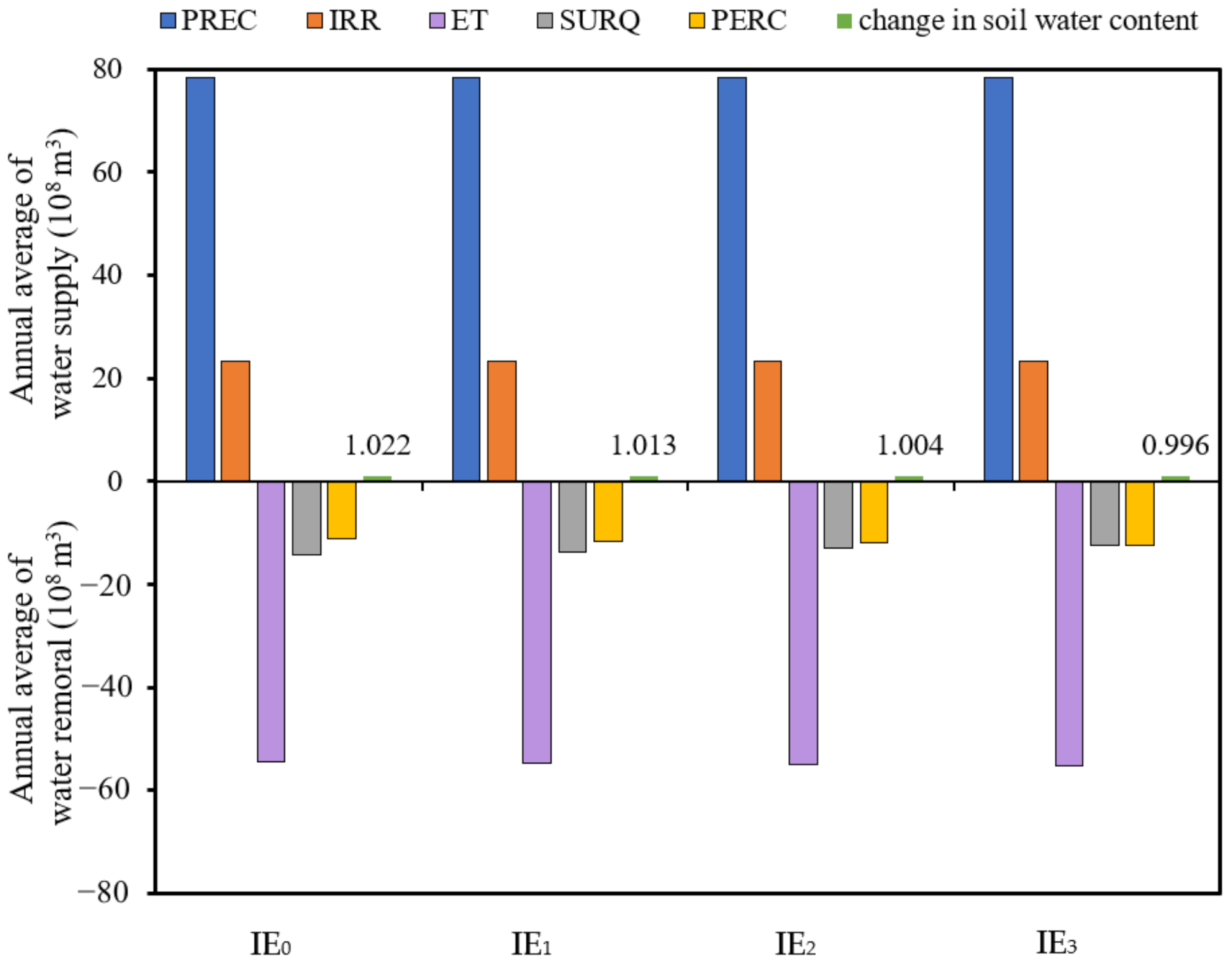
3.2.3. Evaluation Impacts of Water Saving Irrigation on Hydrological Water Balance
4. Conclusions
- The overall result of the model performance for the entire study area was satisfactory judging by the R2, NSE and PBIAS metrics in both the calibration and validation period. It indicates that it is a good alternative method to introducing the satellite-based ET datasets to calibrating the SWAT model when hydro-meteorological are missing.
- Improving the EUCIW was helpful in decreasing SURQ but increasing PERC, while it had no obvious effect on ET.
- The main inputs of the irrigation area were PREC and IRR, while the main output was ET. The effect of the improvement of the water-saving degree on the hydrological cycle system was mainly during the periods when IRR was greater than PREC.
- With the improvement of the water-saving degree, more input water resources (including PREC and IRR) were resupplied to groundwater through increasing PERC and less were converted to SURQ. The decrease in the value of the change in soil water content showed that the improvement of the water-saving degree plays a positive role on maintaining the sustainable development of water resources in irrigated areas.
Author Contributions
Funding
Institutional Review Board Statement
Informed Consent Statement
Data Availability Statement
Acknowledgments
Conflicts of Interest
References
- Carroll, S.; Liu, A.; Dawes, L.; Hargreaves, M.; Goonetilleke, A. Role of Land Use and Seasonal Factors in Water Quality Degradations. Water Resour. Manag. 2013, 27, 3433–3440. [Google Scholar] [CrossRef] [Green Version]
- McDonald, R.; Weber, K.; Padowski, J.; Flörke, M.; Schneider, C.; Green, P.A.; Gleeson, T.; Eckman, S.; Lehner, B.; Balk, D.; et al. Water on an urban planet: Urbanization and the reach of urban water infrastructure. Glob. Environ. Chang. 2014, 27, 96–105. [Google Scholar] [CrossRef] [Green Version]
- Zhang, J.S.; Xu, J.X.; Zhang, Y.Q.; Wang, M.Q.; Cheng, Z.S. Water resources utilization and eco-environmental safety in Northwest China. J. Geogr. Sci. 2006, 16, 277–285. [Google Scholar] [CrossRef]
- Gonçalves, J.M.; Pereira, L.S.; Fang, S.X.; Dong, B. Modelling and multicriteria analysis of water-saving scenarios for an irrigation district in the upper Yellow River Basin. Agric. Water Manag. 2007, 94, 93–108. [Google Scholar] [CrossRef]
- Han, D.; Song, X.; Currell, M.J.; Cao, G.; Zhang, Y.; Kang, Y. A survey of groundwater levels and hydrogeochemistry in irrigated fields in the Karamay Agricultural Development Area, northwest China: Implications for soil and groundwater salinity resulting from surface water transfer for irrigation. J. Hydrol. 2011, 405, 217–234. [Google Scholar] [CrossRef]
- Piao, S.; Ciais, P.; Huang, Y.; Shen, Z.; Peng, S.; Li, J.; Zhou, L.; Liu, H.; Ma, Y.; Ding, Y.; et al. The impacts of climate change on water resources and agriculture in China. Nature 2010, 467, 43–51. [Google Scholar] [CrossRef]
- Xu, X.; Huang, G.; Qu, Z.; Pereira, L.S. Assessing the groundwater dynamics and impacts of water-saving in the Hetao Irrigation District, Yellow River basin. Agric. Water Manag. 2010, 98, 301–313. [Google Scholar] [CrossRef]
- Belder, P.; Bouman, B.; Cabangon, R.; Guoan, L.; Quilang, E.; Yuanhua, L.; Spiertz, J.; Tuong, T. Effect of water-saving irrigation on rice yield and water use in typical lowland conditions in Asia. Agric. Water Manag. 2004, 65, 193–210. [Google Scholar] [CrossRef]
- Mermoud, A.; Tamini, T.D.; Yacouba, H. Impacts of different irrigation schedules on the water balance components of an onion crop in a semi-arid zone. Agric. Water Manag. 2005, 77, 282–295. [Google Scholar] [CrossRef]
- Yue, W.F.; Liu, X.Z.; Wang, T.J.; Chen, X.H. Impacts of water-saving on groundwater balance in a large scale arid irrigation district, Northwest China. Irrig. Sci. 2016, 34, 297–312. [Google Scholar] [CrossRef]
- Jiang, L.; Xue, L.; Liu, Y.; Li, W.; Chi, Y. Effects of water-saving irrigation on groundwater in arid basin based on MIKE SHE model. J. Irrig. Drain. 2016, 35, 59–65. [Google Scholar]
- Zhang, Z.; Hu, H.; Tian, F.; Yao, X.; Sivapalan, M. Groundwater dynamics under water-saving irrigation and implications for sustainable water management in an oasis: Tarim River basin of western China. Hydrol. Earth Syst. Sci. 2014, 18, 3951–3967. [Google Scholar] [CrossRef] [Green Version]
- Uniyal, B.; Jha, M.K.; Verma, A.K. Parameter identification and uncertainty analysis for simulating streamflow in a river basin of Eastern India. Hydrol. Process. 2015, 29, 3744–3766. [Google Scholar] [CrossRef]
- Easton, Z.M.; Fuka, D.R.; Walter, M.T.; Cowan, D.M.; Schneiderman, E.M.; Steenhuis, T.S. Re-conceptualizing the soil and water assessment tool (SWAT) model to predict runoff from variable source areas. J. Hydrol. 2008, 348, 279–291. [Google Scholar] [CrossRef]
- Manaswi, C.M.; Thawait, A.K. Application of soil and water assessment tool for runoff modeling of Karam River basin in Madhya Pradesh. Int. J. Sci. Eng. Technol. 2014, 3, 529–532. [Google Scholar]
- Sun, C.; Ren, L. Assessment of surface water resources and evapotranspiration in the Haihe River basin of China using SWAT model. Hydrol. Process. 2012, 27, 1200–1222. [Google Scholar] [CrossRef]
- Gao, Y.; Long, D. Intercomparison of remote sensing-based models for estimation of evapotranspiration and accuracy assessment based on SWAT. Hydrol. Process. 2008, 22, 4850–4869. [Google Scholar] [CrossRef]
- Chen, F.; Crow, W.T.; Starks, P.J.; Moriasi, D.N. Improving hydrologic predictions of a catchment model via assimilation of surface soil moisture. Adv. Water Resour. 2011, 34, 526–536. [Google Scholar] [CrossRef]
- Li, M.; Ma, Z.; Du, J. Regional soil moisture simulation for Shaanxi Province using SWAT model validation and trend analysis. Sci. China Earth Sci. 2010, 53, 575–590. [Google Scholar] [CrossRef]
- Narasimhan, B.; Srinivasan, R.; Arnold, J.G.; Di Luzio, M. Estimation of long-term soil moisture using a distributed parameter hydrologic model and verification using remotely sensed data. Trans. ASAE 2005, 48, 1101–1113. [Google Scholar] [CrossRef]
- Cheema, M.; Immerzeel, W.; Bastiaanssen, W. Spatial Quantification of Groundwater Abstraction in the Irrigated Indus Basin. Ground Water 2014, 52, 25–36. [Google Scholar] [CrossRef] [PubMed] [Green Version]
- Zhang, X.; Ren, L.; Kong, X. Estimating spatiotemporal variability and sustainability of shallow groundwater in a well-irrigated plain of the Haihe River basin using SWAT model. J. Hydrol. 2016, 541, 1221–1240. [Google Scholar] [CrossRef]
- Xie, X.; Cui, Y. Development and test of SWAT for modeling hydrological processes in irrigation districts with paddy rice. J. Hydrol. 2011, 396, 61–71. [Google Scholar] [CrossRef]
- Goswami, S.; Kar, S. Simulation of water cycle components in the Narmada River basin by forcing SWAT model with CFSR data. Meteorol. Hydrol. Water Manag. 2017, 6, 13–25. [Google Scholar] [CrossRef]
- Jin, X.; Jin, Y. Calibration of a Distributed Hydrological Model in a Data-Scarce Basin Based on GLEAM Datasets. Water 2020, 12, 897. [Google Scholar] [CrossRef] [Green Version]
- Wang, Y.; Brubaker, K. Implementing a nonlinear groundwater module in the soil and water assessment tool (SWAT). Hydrol. Process. 2013, 28, 3388–3403. [Google Scholar] [CrossRef]
- Fisher, J.B.; Tu, K.P.; Baldocchi, D.D. Global estimates of the land–atmosphere water flux based on monthly AVHRR and ISLSCP-II data, validated at 16 FLUXNET sites. Remote Sens. Environ. 2008, 112, 901–919. [Google Scholar] [CrossRef]
- Mu, Q.; Zhao, M.; Running, S.W. Improvements to a MODIS global terrestrial evapotranspiration algorithm. Remote Sens. Environ. 2011, 115, 1781–1800. [Google Scholar] [CrossRef]
- Miralles, D.G.; Holmes, T.; De Jeu, R.A.M.; Gash, J.H.; Meesters, A.G.C.A.; Dolman, A. Global land-surface evaporation estimated from satellite-based observations. Hydrol. Earth Syst. Sci. 2011, 15, 453–469. [Google Scholar] [CrossRef] [Green Version]
- Immerzeel, W.; Droogers, P. Calibration of a distributed hydrological model based on satellite evapotranspiration. J. Hydrol. 2008, 349, 411–424. [Google Scholar] [CrossRef]
- Emam, A.R.; Kappas, M.; Linh, N.H.K.; Renchin, T. Hydrological Modeling and Runoff Mitigation in an Ungauged Basin of Central Vietnam Using SWAT Model. Hydrology 2017, 4, 16. [Google Scholar] [CrossRef] [Green Version]
- Ha, L.T.; Bastiaanssen, W.G.M.; Van Griensven, A.; Van Dijk, A.I.J.M.; Senay, G.B. Calibration of Spatially Distributed Hydrological Processes and Model Parameters in SWAT Using Remote Sensing Data and an Auto-Calibration Procedure: A Case Study in a Vietnamese River Basin. Water 2018, 10, 212. [Google Scholar] [CrossRef] [Green Version]
- Parajuli, P.B.; Jayakody, P.; Ouyang, Y. Evaluation of Using Remote Sensing Evapotranspiration Data in SWAT. Water Resour. Manag. 2018, 32, 985–996. [Google Scholar] [CrossRef]
- Arnold, J.G.; Srinivasan, R.; Muttiah, R.S.; Williams, J.R. Large area hydrologic modeling and assessment part I: Model development. JAWRA J. Am. Water Resour. Assoc. 1998, 34, 73–89. [Google Scholar] [CrossRef]
- Neitsch, S.L.; Arnold, J.G.; Kiniry, J.R.; Williams, J.R. Soil and Water Assessment Tool Theoretical Documentation Version 2009; Texas Water Resources Institute Technical Report No.406; Texas Water Resources Institute: College Station, TX, USA, 2011. [Google Scholar]
- Gassman, P.W.; Reyes, M.R.; Green, C.H.; Arnold, J.G. The Soil and Water Assessment Tool: Historical Development, Applications, and Future Research Directions. Trans. ASABE 2007, 50, 1211–1250. [Google Scholar] [CrossRef] [Green Version]
- Fischer, G.; Nachtergaele, F.; Prieler, S.; van Velthuizen, H.T.; Verelst, L.; Wiberg, D. Global Agro-Ecological Zones Assessment for Agriculture (GAEZ 2008); IIASA: Laxenburg, Austria; FAO: Rome, Italy, 2008. [Google Scholar]
- Guo, A.; Jiang, D.; Zhong, F.; Ding, X.; Song, X.; Cheng, Q.; Zhang, Y.; Huang, C. Prediction of Technological Change under Shared Socioeconomic Pathways and Regional Differences: A Case Study of Irrigation Water Use Efficiency Changes in Chinese Provinces. Sustainability 2019, 11, 7103. [Google Scholar] [CrossRef] [Green Version]
- Feng, B.Q. Study on the Evaluation and Management of Irrigation Water Use Efficiency for Different Scales in Countrywide; China Institute of Water Resources & Hydropower Research (IWHR): Beijing, China, 2013. [Google Scholar]
- Abbaspour, K.C.; Johnson, C.A.; Van Genuchten, M.T. Estimating uncertain flow and transport parameters using a sequential uncertainty fitting procedure. Vadose Zone J. 2004, 3, 1340–1352. [Google Scholar] [CrossRef]
- Abbaspour, K.C.; Yang, J.; Maximov, I.; Siber, R.; Bogner, K.; Mieleitner, J.; Zobrist, J.; Srinivasan, R. Modelling hydrology and water quality in the pre-alpine/alpine Thur watershed using SWAT. J. Hydrol. 2007, 333, 413–430. [Google Scholar] [CrossRef]
- Abbaspour, K.C. SWAT-CUP 2012. SWAT Calibration and Uncertainty Program—A User Manual; Eawag and Swiss Federal Institute of Aqutic Science and Technology: Dübendorf, Switzerland, 2014. [Google Scholar]
- Moriasi, D.N.; Arnold, J.G.; Van Liew, M.W.; Bingner, R.L.; Harmel, R.D.; Veith, T.L. Model Evaluation Guidelines for Systematic Quantification of Accuracy in Watershed Simulations. Trans. ASABE 2007, 50, 885–900. [Google Scholar] [CrossRef]
- Gupta, H.V.; Soroosh, S.; Patrice, O.Y. Status of Automatic Calibration for Hydrologic Models: Comparison with Multilevel Expert Calibration. J. Hydrol. Eng. 1999, 4, 135–143. [Google Scholar] [CrossRef]
- Van Liew, M.W.; Veith, T.L.; Bosch, D.D.; Arnold, J.G. Suitability of SWAT for the Conservation Effects Assessment Project: Comparison on USDA Agricultural Research Service Watersheds. J. Hydrol. Eng. 2007, 12, 173–189. [Google Scholar] [CrossRef] [Green Version]
- Schuol, J.; Abbaspour, K.C.; Srinivasan, R.; Yang, H. Estimation of freshwater availability in the West African sub-continent using the SWAT hydrologic model. J. Hydrol. 2008, 352, 30–49. [Google Scholar] [CrossRef]
- Milewski, A.; Sultan, M.; Yan, E.; Becker, R.; Abdeldayem, A.; Soliman, F.; Gelil, K.A. A remote sensing solution for estimating runoff and recharge in arid environments. J. Hydrol. 2009, 373, 1–14. [Google Scholar] [CrossRef]
- Rajib, A.; Merwade, V.; Yu, Z. Multi-objective calibration of a hydrologic model using spatially distributed remotely sensed/in-situ soil moisture. J. Hydrol. 2016, 536, 192–207. [Google Scholar] [CrossRef] [Green Version]
- Zhang, Q.; Yue, Q.H.; Dong, X.H.; Yang, B.Y.; Wei, C.; Yu, D.; Zang, T. The application of remote sensing data to the SWAT model enhances its accuracy of evapotranspiration. J. Water Resour. Water Eng. 2020, 31, 37–44. [Google Scholar]
- He, S.; Tian, J.; Zhang, Y. Verification and comparison of three high-resolution surface evapotranspiration products in North China. Resour. Sci. 2020, 42, 2035–2046. [Google Scholar] [CrossRef]
- Ahmadzadeh, H.; Morid, S.; Delavar, M.; Srinivasan, R. Using the SWAT model to assess the impacts of changing irrigation from surface to pressurized systems on water productivity and water saving in the Zarrineh Rud catchment. Agric. Water Manag. 2016, 175, 15–28. [Google Scholar] [CrossRef]
- Dai, F.G.; Cai, H.J.; Liu, X.; Liang, H.W. Simulation of effect of water-saving renovation on spatial distribution of groundwater in Jinghui Canal irrigation area. J. Drain. Irrig. Mach. Eng. 2013, 31, 729–736. [Google Scholar]
- Clemmens, A.J.; Allen, R.G. Impact of Agricultural Water Conservation on Water Availability; American Society of Civil Engineers (ASCE): Reston, VA, USA, 2005; pp. 1–14. [Google Scholar]


| Irrigation Year | Canal Irrigation Quantity (104 m3) | Well Irrigation Quantity (104 m3) | EUCIW0 * | ||||
|---|---|---|---|---|---|---|---|
| Winter | Spring | Summer | Winter | Spring | Summer | ||
| 2001 | 4240 | 4206 | 2950 | 4079 | 4047 | 2838 | 0.522 |
| 2002 | 5268 | 3523 | 2770 | 5703 | 3814 | 2998 | 0.524 |
| 2003 | 3551 | 2988 | 2105 | 4266 | 3590 | 2529 | 0.523 |
| 2004 | 5186 | 3543 | 2596 | 5203 | 3554 | 2604 | 0.525 |
| 2005 | 3855 | 4866 | 3712 | 3581 | 4520 | 3448 | 0.528 |
| 2006 | 4858 | 4350 | 3445 | 4704 | 4212 | 3336 | 0.531 |
| 2007 | 5470 | 3040 | 1123 | 5894 | 3276 | 1210 | 0.532 |
| 2008 | 5486 | 3059 | 4586 | 5209 | 2904 | 4355 | 0.535 |
| 2009 | 5298 | 4828 | 3619 | 4221 | 3846 | 2883 | 0.535 |
| 2010 | 6030 | 4038 | 3801 | 4630 | 3101 | 2919 | 0.537 |
| Simulation Result | Absolute Value of PBIAS | NSE |
|---|---|---|
| Very good | |PBIAS| ≤ 10% | NSE > 0.75 |
| Good | 10% < |PBIAS| ≤ 15% | 0.65 < NSE ≤ 0.75 |
| Satisfactory | 15% < |PBIAS| ≤ 25% | 0.50 < NSE ≤ 0.65 |
| Unsatisfactory | |PBIAS| > 25% | NSE ≤ 0.50 |
| Parameter Name * | Physical Meaning | t-Stat | p-Value | Fitted Value |
|---|---|---|---|---|
| V_GWQMN.gw | Threshold depth of water in the shallow aquifer required for return flow to occur (mm) | 5.00 | 0.00 | 2675 |
| V_CANMX.hru | Maximum canopy storage (mm) | 3.39 | 0.00 | 51.50 |
| V_REVAPMN.gw | Threshold depth of water in the shallow aquifer for “revap” to occur (mm) | 3.33 | 0.00 | 122.50 |
| V_GW_DELAY.gw | Groundwater delay (days) | 3.32 | 0.00 | 127.50 |
| V_SURLAG.bsn | Surface runoff lag time (days) | 3.04 | 0.00 | 22.48 |
| V_GW_REVAP.gw | Groundwater “revap” coefficient | 2.61 | 0.01 | 0.06 |
| V_ALPHA_BF.gw | Baseflow alpha factor (days) | 2.11 | 0.04 | 0.66 |
| V_EPCO.hru | Plant uptake compensation factor | 1.33 | 0.19 | 0.65 |
| R_SOL_Z.sol | Depth from soil surface to bottom of layer (mm) | −0.56 | 0.58 | −0.24 |
| R_SOL_K.sol | Saturated hydraulic conductivity (mm/h) | 0.49 | 0.62 | 0.02 |
| R_SOL_ALB.sol | Moist soil albedo | 0.38 | 0.70 | 0.28 |
| R_SOL_AWC.sol | Available water capacity of the soil layer (mm/mm) | 0.35 | 0.72 | −0.20 |
| V_OV_N.hru | Manning’s “n” value for overland flow | 0.30 | 0.77 | 28.35 |
| R_CN2.mgt | SCS runoff curve number for moisture condition 2 | 0.24 | 0.81 | −0.14 |
| R_SOL_BD.sol | Moist bulk density (g/cm3) | 0.23 | 0.82 | 0.48 |
| V_ESCO.hru | Soil evaporation compensation factor | 0.15 | 0.88 | 0.51 |
Publisher’s Note: MDPI stays neutral with regard to jurisdictional claims in published maps and institutional affiliations. |
© 2021 by the authors. Licensee MDPI, Basel, Switzerland. This article is an open access article distributed under the terms and conditions of the Creative Commons Attribution (CC BY) license (https://creativecommons.org/licenses/by/4.0/).
Share and Cite
Zhang, M.; Wang, X.; Zhou, W. Effects of Water-Saving Irrigation on Hydrological Cycle in an Irrigation District of Northern China. Sustainability 2021, 13, 8488. https://doi.org/10.3390/su13158488
Zhang M, Wang X, Zhou W. Effects of Water-Saving Irrigation on Hydrological Cycle in an Irrigation District of Northern China. Sustainability. 2021; 13(15):8488. https://doi.org/10.3390/su13158488
Chicago/Turabian StyleZhang, Manfei, Xiao Wang, and Weibo Zhou. 2021. "Effects of Water-Saving Irrigation on Hydrological Cycle in an Irrigation District of Northern China" Sustainability 13, no. 15: 8488. https://doi.org/10.3390/su13158488
APA StyleZhang, M., Wang, X., & Zhou, W. (2021). Effects of Water-Saving Irrigation on Hydrological Cycle in an Irrigation District of Northern China. Sustainability, 13(15), 8488. https://doi.org/10.3390/su13158488