Remaining Useful Life Prediction-Based Maintenance Decision Model for Stochastic Deterioration Equipment under Data-Driven

Abstract

Currently, the Remaining Useful Life (RUL) prediction accuracy of stochastic deterioration equipment is low. Existing researches did not consider the impact of imperfect maintenance on equipment degradation and maintenance decisions. Therefore, this paper proposed a remaining useful life prediction-based maintenance decision model under data-driven to extend equipment life, promoting sustainable development. The stochastic degradation model was established based on the nonlinear Wiener process. A combination of real-time update and offline estimation estimated the degradation model’s parameters and deduced the equipment’s RUL distribution. Based on the RUL prediction results, we established a maintenance decision model with the lowest long-term cost rate as the goal. Case analysis shows that the model proposed in this paper can improve the accuracy of RUL prediction and realize equipment sustainability.

1. Introduction

With the advancement of science and technology, the requirements for equipment reliability are getting higher and higher. The health management of equipment is an essential factor that determines the sustainable development of enterprises and improves production efficiency [1,2]. However, the complex working environment gradually reduces the equipment’s Remaining Useful Life (RUL) and reliability, leading to serious safety accidents [3]. At present, preventive maintenance is still the primary maintenance method for stochastic deterioration equipment, and there is a phenomenon of over or under maintenance [4]. With the rapid development of Sensor technology [5], Data mining [6], and Intelligent algorithms [7], Prognostics and Health Management (PHM) has gradually become the main management methods for complex equipment systems [8], which has attracted the attention of many scholars at home and abroad [9,10,11,12].

PHM technology mainly includes RUL prediction and health management. At present, most researches focus on the RUL prediction. The main methods include degradation mechanism, [13,14,15], data-driven, and hybrid models [16,17]. The model method based on the equipment degradation mechanism requires an in-depth understanding of the physical principles of the equipment, and the actual complex working environment limits its development [18,19]. The data-driven method is widely used in RUL estimation due to its flexibility [20], mainly including neural network-based method, regression-based method [21], random filtering-based method [22,23], and random process-based method. Han, C. et al. [24] proposed a mobile convolutional neural network (TCNN) to learn domain invariant features. The trained TCNN can be used to predict RUL by feeding data. Chen, Z. et al. [25] proposed an attention-based deep learning framework to predict the RUL of the equipment. Meng, M. et al. [26] proposed a convolution-based long short-term memory (CLSTM) network to predict the RUL of rotating machinery. Unlike the literature [25], the proposed network performs convolution operations on both the input state transition and state transition of LSTM, which retains the advantages of LSTM and integrates time-frequency characteristics.

However, the above method requires a large amount of status monitoring data to model the degradation process. Furthermore, due to the complex operating environment of the equipment, the error in the measurement data and other factors cannot guarantee the accuracy of the results. Considering the uncertainty of life prediction, the modeling method based on a stochastic degradation process proposed by Nozer, D. [27] has been recognized as an effective method for equipment health management and remaining life prediction [28,29,30]. In addition, many scholars have established random degradation models based on the Gamma process [31,32], Gaussian process [33,34], Inverse-Gaussian process [35], and Wiener process. Both the Gamma process and the Gaussian process are only applicable to the monotonic degradation process. However, the Wiener process can describe the non-monotonic process of equipment degradation and has become a research hotspot [36,37]. Li, N. et al. [38] designed an RUL prediction method based on Wiener Process Model, which is based on the Maximum Likelihood Estimation (UMLE) algorithm to predict RUL. Man, J. et al. [39] established a random degraded signal model based on the Wiener process with drift and proposed a joint model and a Markov model of the Wiener process. Wang, H. et al. [40] proposed an improved Wiener process model for RUL prediction, in which drift, and diffusion parameters are obtained by real-time updates of monitoring data. Liu, D. et al. [41] proposed a reliability estimation and degradation modeling method based on the Wiener process and evidence variables. By applying evidence variables to describe the model parameters, the Wiener process is combined with evidence theory. The above studies are mainly based on the Wiener process to predict the remaining life of the equipment, and there are few studies on the maintenance decisions taken from the prediction results. Zhang, M. [42] established an imperfect maintenance model based on Wiener stochastic process and considered the impact of degradation rate on maintenance. Liu, B. et al. [43] developed an imperfect maintenance strategy for task-oriented systems, established a random equipment degradation model based on the Wiener degradation process. They adopted preventive replacement and corrective replacement strategies to establish a decision-making model. Based on the Wiener process, Pei, H. et al. [44] proposed a performance degradation and maintenance decision model that considers imperfect maintenance. They adopted a regular maintenance strategy and comprehensively consider the impact of equipment degradation and degradation rate. However, the above models describe the linear degradation process without considering the nonlinear degradation characteristics. The preventive threshold is specified in advance, resulting in inaccurate decision-making results. Wang, Z. et al. [45] used the nonlinear Wiener process and the homogeneous Poisson process to model the cumulative effect of equipment, thereby improving the accuracy of RUL prediction. However, this model does not study equipment maintenance decisions and assumes that the number of imperfect repairs is unlimited. Therefore, Chen, Y. et al. [46] used nonlinear Wiener process and non-homogeneous Poisson process based on literature [45] to establish an imperfect decision-making model that satisfies the upper limit of the number of repairs. However, this model adopts the maximum likelihood method for parameter estimation and cannot update the parameters according to the equipment’s real-time data, making the predicted result inaccurate and affects the accuracy of maintenance decision.

In summary, the current RUL prediction methods can hardly reflect the true degradation process of equipment. Researchers does not consider the impact of imperfect maintenance on equipment degradation and maintenance decisions. Therefore, this paper establishes the equipment maintenance decision model based on the RUL prediction under the data-driven method. First, we use the nonlinear Wiener process to establish the equipment degradation model, and the method of online parameter update is introduced. The offline estimation and online update are combined to estimate the parameters of the degradation model, and the RUL distribution of the equipment is derived. Then, based on the result of the RUL prediction, an imperfect maintenance strategy with limited maintenance times is adopted. The maintenance decision model is established with the lowest long-term cost rate as the goal. Finally, taking the bearing as an example, we compared the validity and accuracy of the model.

2. Problem Description and Model Assumptions

2.1. Problem Description

Maintenance includes perfect maintenance, imperfect maintenance and minor repairs. It is not easy to achieve perfect maintenance in the actual production process, especially in the face of complex equipment. Most projects use imperfect maintenance, and maintenance activities cannot restore the equipment to a brand new state. With the development of sensing technology, we can detect the operating data of the equipment, obtain the current degradation state, and provide a basis for maintenance. Based on the idea of imperfect maintenance, this paper adopts a restrictive maintenance strategy. When equipment degradation reaches a certain threshold, it will be maintained. However, it cannot be restored as new and equipment maintenance does not increase indefinitely. As the number of maintenance increases, equipment degradation increases until it completely fails. Figure 1 shows the equipment degradation process.

In Figure 1, the abscissa is the equipment operating time t, the ordinate is the equipment degradation $X\left(t\right)$, $\omega$ is the failure threshold, and ${\omega }_p$ is the maintenance threshold.

2.2. Model Assumptions

The assumptions of this article mainly include the following points:

(1)

Preventive maintenance does not affect the degradation mechanism of the equipment itself and can slow down the process of equipment degradation. However, preventive maintenance activities are not unlimited. When the number of maintenance reaches the prescribed upper limit N, maintenance activities will no longer be carried out.

(2)

The status value of each period can be obtained through the detection method, and the replacement and repair time of the equipment under any maintenance means is ignored.

(3)

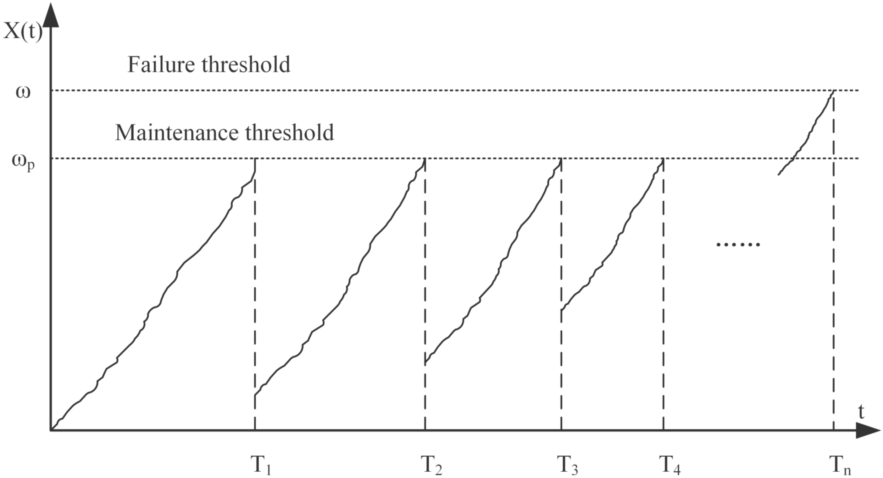
When equipment degradation is less than the preventive maintenance threshold ${\omega }_p$, no maintenance, and the equipment usually operates.

(4)

When equipment degradation is greater than the preventive maintenance threshold ${\omega }_p$, but the number of maintenance does not exceed N, we take preventive maintenance.

(5)

When the overall degradation exceeds the failure threshold $\omega$, the system will fail, and time-sensitive replacement will be adopted.

3. Model Building

3.1. Non-Linear Drift Wiener Degradation Model

The mathematical expression of the Wiener process [47] can be expressed as:

$$X\left(t\right)=X\left(0\right)+\mu t+\sigma B\left(t\right)$$

(1)

where, $X\left(t\right)$ is the degradation of the equipment at time t. $X\left(0\right)$ is the degradation of the equipment at time 0. $\mu$ is the drift coefficient. $\sigma$ is the diffusion coefficient. $B\left(t\right)$ is the standard Brownian motion.

The Wiener process expression of nonlinear drift can be written as [48]:

$$X\left(t\right)=X\left(0\right)+\alpha {\int }_0^t\mu (\tau ,\beta )d\tau +\sigma B\left(t\right)$$

(2)

where, $\alpha {\int }_0^t\mu (\tau ,\beta )d\tau$ represents the average cumulative effect of the equipment degradation process, which is the nonlinear drift of the degradation amount. $\alpha$ is a random parameter, $\beta$ and $\sigma$ are common parameters, $\alpha \sim N({\mu }_0,{\sigma }_0^2)$. $\alpha$ and $B\left(t\right)$ are statistically independent.

The Wiener degradation process based on imperfect maintenance can be expressed as [44]:

$$X\left(t\right)=X_i+\alpha {\int }_{T_i}^t\mu (\tau ,\beta )d\tau +\sigma B(t-T_i)$$

(3)

where, $X_i$ is the degradation amount of the equipment after i maintenance, $i(0\le i\le N)$. N is the total number of maintenance. The probability density of $X_i$ satisfies:

$$f\left(X_i\right)=\frac{a^{i-1}b}{1-exp\left(a^{i-1}b{\omega }_p\right)}exp[\frac{a^{i-1}b({\omega }_p-X_i)}{{\omega }_p}{X}_i^{\prime }]$$

(4)

3.2. RUL Prediction Model

Based on the first arrival time, the equipment degradation life T represented by the Wiener process with nonlinear drift is defined as [49]:

$$T=inft,X\left(t\right)\ge \omega \left|X\right(0)<\omega$$

(5)

where, $\omega$ is the known failure threshold.

In order to obtain the probability density of the analytical form of the equipment life T, considering the randomness of the parameters, redefine the probability density function of the life T can be given as:

$$f_{T|\alpha }\left(t\right|\alpha )\cong \frac{\omega -\alpha {\int }_{T_i}^t\mu (\tau ,\beta )d\tau +\sigma B\left(t\right)}{\sigma t\sqrt{2\pi t}}exp\{\frac{{[\omega -\alpha {\int }_{T_i}^t\mu (\tau ,\beta )d\tau ]}^2}{2{\sigma }^{2}t}\}$$

(6)

The unconditional total probability density function of life T is $f_T\left(t\right)$, and the total probability formula can be derived as:

$$f_T\left(t\right)={\int }_{\mathsf{\Phi }}{f}_{t|\alpha }f\left(\alpha \right)d\alpha$$

(7)

where, $f_T$ and $\mathsf{\Phi }$ are the probability density function and parameter space of random parameters.

Through the probability density of life T, the probability density of the RUL of equipment degradation can be obtained. Let $t_n$ be the current time and $l_n$ be the remaining life of the current time. If the equipment reaches the failure threshold for the first time at time t, the actual remaining life is $l_n=t-t_n$. Based on the Wiener process, we can get:

$$X\left(t\right)-X\left(t_n\right)=X\left(0\right)+\alpha {\int }_{t_n}^t\mu (\tau ,\beta )d\tau +\sigma B\left(l_n\right)$$

(8)

From Equations (6)–(8), we know that the probability density function of the remaining life of the degraded equipment at time $t_n$ can be written as:

$$\begin{array}{cc}\hfill f_{L_n}\left(l_n\right)& \cong \frac{1}{\sqrt{2\pi l_n^2[{\sigma }_{\alpha ,n}^2{(\alpha {\int }_{t_n}^t\mu (\tau ,\beta )d\tau )}^2+{\sigma }^2{l}_n]}}\hfill \\ & \{\omega -x_n-[\alpha {\int }_{t_n}^t\mu (\tau ,\beta )d\tau -\mu (l_n+t_n,\beta )l_n]\hfill \\ & \frac{{\sigma }_{\alpha ,n}^2(\omega -x_n{\int }_{t_n}^t\mu (\tau ,\beta )d\tau )+{\mu }_{\alpha ,n}{\sigma }^2{l}_n}{{\sigma }_{\alpha ,n}{({\int }_{t_n}^t\mu (\tau ,\beta )d\tau )}^2+{\sigma }^2{l}_n}\}\hfill \\ & exp\{-\frac{{[\omega -x_n-{\mu }_{\alpha ,n}{\int }_{t_n}^t\mu (\tau ,\beta )d\tau ]}^2}{2[{\sigma }_{\alpha ,n}{({\int }_{t_n}^t\mu (\tau ,\beta )d\tau )}^2+{\sigma }^2{l}_n]}\}\hfill \end{array}$$

(9)

where, ${\mu }_{\alpha ,n}$ and ${\sigma }_{\alpha ,n}^2$ are the mean value and variance of the random parameter $\alpha$ obtained after the update at time $t_n$, respectively. $x_n$ is the degradation observation of the degraded equipment at time $t_n$.

3.3. Maintenance Decision Model

This paper takes the lowest long-term cost rate as the decision-making goal, and uses the maintenance threshold as the decision variable to establish a maintenance decision-making model. According to related theories [50], the average cost rate in the life cycle can be expressed as:

$$C^{\infty }=\underset{t\to +\infty }{lim}C\left(t\right)=\frac{E\left[C\right]}{E\left[T\right]}$$

(10)

where, $C^{\infty }$ is the average cost rate. $E\left[C\right]$ is the average cost, and $E\left[T\right]$ is the average life cycle. The total cost includes inspection cost $C_I$, preventive maintenance cost $C_M$, preventive replacement cost $C_P$, failure replacement cost $C_S$, and $C_I<C_M<C_P<C_S$ The total cost can be expressed as:

$$C^{\infty }=\frac{C_{I}E\left[N_I\right]+C_{M}E\left[N_M\right]+C_P{P}_P+C_S{P}_S}{E\left[T\right]}$$

(11)

$N_I$ is the number of inspections. $N_M$ is the number of maintenance. $P_P$ is the probability of preventive replacement of the equipment. $P_S$ is the probability of failure replacement of the equipment.

The equipment inspection time interval is $\Delta t$, when the amount of degradation after detection meets $0\le X(d_i\Delta t)<{\omega }_p$, and no maintenance measures are taken. When the amount of degradation after detection meets ${\omega }_p\le X(d_i\Delta t)<\omega$, preventive maintenance is taken. When it is detected that the amount of equipment degradation meets ${\omega }_p\le X[(k+1)\Delta t]<\omega ,(K\ge N)$ after completing N maintenance, preventive replacement is adopted. When the equipment has undergone N preventive maintenance, it is detected that the degradation amount satisfies $\omega \le X\left[\right(k+1)\Delta t]$ in the interval $(k\Delta t,(k+1)\Delta t)$, and the failure replacement is adopted.

The maintenance process is shown in Figure 2.

3.3.1. Preventive Replacement

Assuming that the time of the i-th maintenance is $d_i\Delta t$, the probability of preventive maintenance of the equipment at time $d_i\Delta t$ can be expressed as [51]:

$$\begin{array}{cc}\hfill P(d_i\Delta t)& ={\int }_0^{{\omega }_p}\{1-F_{i-1,{\omega }_p}[(d_i-(d_i-1))\Delta t|X_{i-1}]\hfill \\ \hfill & {\int }_{X_{i-1}}^{{\omega }_p}{f}_{i-1}[x,(d_i-(d_i-1)-1)\Delta t](F_{i-1,{\omega }_p-x}(\Delta t,x|X_{i-1})\hfill \\ \hfill & -F_{i-1,\omega -x}(\Delta t,x|X_{i-1}))dx\}f\left(X_{i-1}\right)d_{X_{i-1}}\hfill \end{array}$$

(12)

where,

$$f_i\left(x\right)=\frac{1}{\sqrt{2\pi {\sigma }^{2}t}}exp[-\frac{{(x-X_i-\alpha {\int }_0^{T_i}{\mu }_i(\tau ,\beta )d\tau )}^2}{2{\sigma }^{2}t}]$$

(13)

$$f_{i,\omega -x}\left(\delta \right|X_i)=\frac{\omega -x}{\sqrt{2\pi {\sigma }^2{\delta }^3}}exp[-\frac{{[\omega -x-(\alpha {\int }_{T_i}^t{\mu }_i(\tau ,\beta )d\tau )\delta ]}^2}{2{\sigma }^2{\delta }^3}]$$

(14)

When the number of maintenance is less than N and the equipment degradation satisfies $X((d_i-1)\Delta t)<{\omega }_p\le X(d_i\Delta t)<\omega$, preventive maintenance is taken. The probability at this time is expressed as:

$$\begin{array}{cc}\hfill P_1(d_i\Delta t)& =P{\omega }_p\le X(d_i\Delta t)<\omega ⌒ X((d_i-1)\Delta t)<{\omega }_p|i\le N\hfill \\ \hfill & =P{\omega }_p\le X((d_i-1)\Delta t)<{\omega }_p\hfill \\ \hfill & -PX((d_i-1)\Delta t)<X(d_i\Delta t)\ge \omega \hfill \\ \hfill & ={\omega }_p ⌒ PX((d_i-1)\Delta t)<\omega ⌒ X(\Delta t)\ge {\omega }_p-X((d_i-1)\Delta t)\hfill \\ & -PX((d_i-1)\Delta t)<X(d_i\Delta t)\ge {\omega }_p ⌒ \omega -X(d_i-1)\Delta t\hfill \end{array}$$

(15)

The expenses incurred at this time can be expressed as:

$$C_1^{\prime }=C_I{N}_I^1+(i-1)C_M$$

(16)

When the number of maintenance exceeds N and the equipment degradation satisfies $X(k\Delta t)<{\omega }_p\le X((k+1)\Delta t)<\omega )$, preventive replacement is adopted. The probability at this time is expressed as:

$$\begin{array}{cc}\hfill P_2(k+1,N)& =PX(k\Delta t)<{\omega }_p\le X((k+1)\Delta t)<\omega |k\ge N\hfill \\ \hfill & =\sum _{i=1}^k[\prod _{i=1}^N{P}_1·PX(k\Delta t)<{\omega }_p\le X((k+1)\Delta t)<\omega |k\ge N]\hfill \\ \hfill & =\sum _{i=1}^k[\prod _{i=1}^N{P}_1{\int }_0^{{\omega }_p}\{1-F_{N,{\omega }_p}\left[(k-d_N\Delta t)\right|X_N{\int }_{X_N}^{{\omega }_p}{f}_N(x,(k-d_N)\Delta t)\hfill \\ \hfill & \left(F_{N,\omega -x}(\Delta t,x)\right|X_N)-\left(F_{N,{\omega }_p-x}(\Delta t,x)\right|X_N)]\}dxf\left(X_N\right)d{X}_N]\hfill \end{array}$$

(17)

After N times of maintenance, the probability of preventive replacement of equipment can be given as:

$$P_P=\sum _{k=N}^{\infty }(k+1,N)P_2$$

(18)

The cost at this time can be expressed as:

$$C_1^{″}=C_I{N}_I^1+N{C}_M+C_P$$

(19)

The total cost of preventive replacement at the end of the life cycle can be written as:

$$C_I=C_1^{\prime }+C_1^{″}$$

(20)

3.3.2. Failure Replacement

When the number of maintenance exceeds N and the equipment degradation satisfies $X(k\Delta t)<{\omega }_p ⌒ \omega \le X((k+1)\Delta t)$, the failure replacement is adopted, and the probability at this time can be expressed as:

$$\begin{array}{cc}\hfill P_S(k+1,N)& =PX(k\Delta t)<{\omega }_p ⌒ \omega X((k+1)\Delta t)|k\ge N\hfill \\ \hfill & =\sum _{i=1}^k[\prod _{i=1}^N{P}_1·PX(k\Delta t)<{\omega }_p ⌒ \omega X((k+1)\Delta t)|k\ge N]\hfill \\ \hfill & =\sum _{i=1}^k[\prod _{i=1}^N{P}_1{\int }_0^{\omega }\{1-F_{N,\omega }\left[(k-d_N\Delta t)\right|X_N{\int }_{X_N}^{\omega }{f}_N(x,(k-d_N)\Delta t)\hfill \\ \hfill & \left(F_{N,\omega -x}(\Delta t,x)\right|X_N)-F_{N,\omega -x}(\Delta t,x)|X_N]\}dxf\left(X_N\right)]\hfill \end{array}$$

(21)

The cost $C_2$ incurred at this time can be given as:

$$C_2=C_I{N}_I^2+N{C}_M+C_p$$

(22)

The total cost of the entire maintenance process can be written as:

$$C=C_1+C_2$$

(23)

The life cycle expectations can be expressed as:

$$E\left(T\right)=\sum _{k=N}^{\infty }\sum _{i=0}^N[(k+1)\Delta t{P}_S]+\sum _{k=N}^{\infty }\left[(k+1)P_P\right]$$

(24)

The number of detections can be written as:

$$E(N_i=\frac{E\left(T\right)}{\Delta t})$$

(25)

The number of maintenance can be expressed as:

$$E\left(N_M\right)=\sum _{k=N}^{\infty }\sum _{i=0}^{N}k{P}_S+\sum _{k=N}^{\infty }N{P}_P$$

(26)

The long-term minimum cost rate of the maintenance decision model can be expressed as:

$$min{C}^{\infty }=min\frac{E\left[C\right]}{E\left[T\right]}$$

(27)

3.4. Parameter Estimation

Traditional parameter estimation methods mainly use offline estimation, which has low accuracy. This paper introduces an online update method that combines offline estimation and online updates to estimate the parameters. Parameter estimation is divided into two steps: (1) Offline estimation: Estimate the standard parameters $\beta$ and $\alpha$ based on the historical data of equipment degradation, and hyperparameters ${\mu }_{\alpha ,0}$ and ${\sigma }_{\alpha ,0}^2$ in the prior distribution of random parameter $\alpha$. (2) Online update: at any time $t_n$ use the actual monitored degradation data to update the parameters in the random parameter $\alpha$ distribution $f\left(\alpha \right)$.

3.4.1. Parameter Offline Estimation

Suppose there are degradation data of M devices of the same type, and the degradation data of the j-th device is $M_j$. Then the degradation amount of the j-th device at the k-th moment is $X\left(t_{j,k}\right)$.

From Equation (2), we can get:

$$X_{j,k}=X\left(0\right)+{\alpha }_0{\int }_0^{t_{j,k}}\mu (\tau ,\beta )d\tau +\sigma B\left(t_{j,k}\right)$$

(28)

where: ${\alpha }_0$ is the prior value of the random parameter $\alpha$, and its distribution is ${\pi }_0\left(\alpha \right)\backsim N({\mu }_{\alpha ,0},{\sigma }_{\alpha ,0}^2)$.

Assume that the degradation data of different degraded equipment is irrelevant, while the data of the same degraded equipment is related. The jth equipment degradation data is $X_j={(X_{j,1},X_{j,2},X_{j,3},\cdots X_{j,M})}^{\prime }$, $X_j$ obeys the multivariate Gaussian distribution, and the mean and covariance can be written as [52]:

$$\begin{array}{cc}\hfill {\mu }_i& ={\mu }_{\alpha ,0}{I}_j\hfill \\ \hfill {\sum }_j& ={\sigma }_0^2{I}_j{I}_j{}^{\prime }+{\sigma }^2{K}_j\hfill \end{array}$$

(29)

$$I_i=({\int }_0^{t_{j,1}}\mu (\tau ,\beta )d\tau ,{\int }_0^{t_{j,2}}\mu (\tau ,\beta )d\tau ,\cdots {\int }_0^{t_{j,M_j}}\mu (\tau ,\beta )d\tau ){}^{\prime }$$

(30)

$$K_j=\left[\begin{array}{cccc}{t}_{j,1}& t_{j,1}& \cdots & t_{j,1}\\ t_{j,1}& t_{j,2}& \cdots & t_{j,1}\\ ⋮& ⋮& \ddots & ⋮\\ t_{j,1}& t_{j,2}& \cdots & t_{j,M_j}\end{array}\right]$$

(31)

From Equation (11), the mean value of $X_j$ is ${\mu }_j={\mu }_{\alpha ,0}{I}_j$, and the covariance matrix $X_j$ can be expressed as:

$${\sum }_j=\left[\begin{array}{cccc}D\left(X_{j,1}\right)& covD(X_{j,1},X_{j,2})& \cdots & covD(X_{j,1},X_{j,M_j})\\ & & \cdots & covD(X_{j,1},X_{j,M_j})\\ & & \ddots & ⋮\\ & & & covD(X_i,X_{j,M_j})\end{array}\right]$$

(32)

The variance $D\left(X_{j,k}\right)$ can be expressed as:

$$\begin{array}{cc}\hfill D\left(X_{j,k}\right)& =D({\alpha }_0{\int }_0^{t_{j,k}}\mu (\tau ,\beta )d\tau +\sigma B\left(t_{j,k}\right))\hfill \\ \hfill & ={\sigma }_{\alpha ,0}^2{[{\int }_0^{t_{j,k}}\mu (\tau ,\beta )d\tau ]}^2+{\sigma }^2{t}_{j,k}\hfill \end{array}$$

(33)

From Equation (12), the likelihood function formed by the degradation data of M degraded devices is:

$$\begin{array}{cc}\hfill \ell \left(\mathsf{\Theta }\right|X_j)& =-\frac{1}{2}ln\left(2\pi \right){\sum }_{j=1}^M{M}_j-\frac{1}{2}{\sum }_{j=1}^{M}ln\left|{\sum }_j\right|\hfill \\ \hfill & =-\frac{1}{2}(X_j-{\mu }_j){}^{\prime }{\sum }_{j=1}^M(X_j-{\mu }_j){}^{\prime }{\sum }_j^{-1}(X_j-{\mu }_j)\hfill \end{array}$$

(34)

where: $\mathsf{\Theta }=({\mu }_{\alpha ,0},{\sigma }_{\alpha ,0},\beta ,\sigma ){}^{\prime }$ is an unknown parameter, and $X_j=(X_1,X_2,\cdots X_M)$ is the degradation data of M devices.

3.4.2. Real-Time Parameter Estimation

For a certain device, at any time $t_k$ during its life, the random parameter $\alpha$ of the degradation model can be estimated from all the data previously observed by the device. Based on Bayesian theory, the posterior parameter distribution of the random parameters of the degradation model at time $t_k$ is as follows [53]:

$$P\left(\alpha \right|x_{1,k})\propto p\left(x_{1,k}\right|\alpha ){\pi }_0\left(\alpha \right)$$

(35)

where, $P\left(\alpha \right|x_{1,k})$ represents the likelihood function under given random parameters, and the prior distribution can be obtained by Equation (17).

Using the basic characteristics of Brownian motion, we can get:

$$P\left(\alpha \right|x_{1,k})=\frac{1}{{\prod }_{q=1}^k\sqrt{2\pi {\sigma }^2(t_q-t_{q-1})}}exp\{-{\sum }_{q=1}^k\frac{{[x_q-x_{q-1}-{\int }_{q-1}^{t_q}\mu (\tau ,\beta )d\tau ]}^2}{2{\sigma }^2(t_q-t_{q-1})}\}$$

(36)

Since $P\left(\alpha \right|x_{1,k})$ and ${\pi }_0$ are both normally distributed, $P\left(x_{1,k}\right|\alpha )$ is also normally distributed. From Equations (18) and (19), it can be seen that the mean and variance of $P\left(x_{1,k}\right|\alpha )$ are expressed as:

$${\mu }_{\alpha ,k}=\frac{\frac{{\mu }_{\alpha ,0}}{{\sigma }_{\alpha ,0}^2}+{\sum }_{q-1}^k\{\frac{{(x_q-x_{q-1}-{\int }_{q-1}^{t_q}\mu (\tau ,\beta )d\tau )}^2}{{\sigma }^2(t_q-t_{q-1})}\}}{{\sum }_{q-1}^k\{\frac{{\left({\int }_{q-1}^{t_q}\mu (\tau ,\beta )d\tau \right)}^2}{{\sigma }^2(t_q-t_{q-1})}\}+\frac{1}{{\sigma }_{\alpha ,0}^2}}$$

(37)

$${\sigma }_{\alpha ,k}^2=\frac{1}{{\sum }_{q-1}^k\{\frac{{\left({\int }_{q-1}^{t_q}\mu (\tau ,\beta )d\tau \right)}^2}{{\sigma }^2(t_q-t_{q-1})}\}+\frac{1}{{\sigma }_{\alpha ,0}^2}}$$

(38)

Incorporating Equations (34), (37) and (38) into Equation (9), the probability density function of the remaining life of the equipment at the moment can be obtained.

4. Case Analysis and Discussion

4.1. Case Analysis

Bearing is a critical component of mechanical equipment. Its primary function is to support the mechanical rotating body, reduce the friction coefficient during its movement, and ensure its rotation accuracy. At present, bearings are widely used in complex equipment such as aerospace, large machinery, and equipment. As a crucial part of significant equipment, bearings develop in high speed, high precision, high reliability and long life. However, the complex and harsh working environment has led to a relatively high failure rate of bearings, affecting the regular operation of the equipment and even causing severe safety accidents. In the actual operation process, people take regular replacement strategy for bearings, which does not extend the remaining service life of the bearings, which is not conducive to sustainable development.

This paper takes bearing as the research object, we use the bearing degradation data of PHM competition [54] as the original data for analysis and calculation. FEMTO-ST Research Institute provides the PHM data set, and the experiment is carried out on the laboratory experimental platform (PRONOSTIA). The sampling frequency is 25.6 kHz, and the original vibration signal changes of the three sets of data of the same bearing during the whole life cycle are shown in Figure 3.

The Root Mean Square (RMS) can reflect the vibration signal well, so we use the RMS as the characteristic signal data. The RMS value of the three sets of data is shown in Figure 4.

The bearing failure threshold after RMS processing is 6. It can be seen from Figure 4, the first set of data and the second set of data have failed. The third set of data has not failed. The first set of data has a longer life cycle. Therefore, this paper selects the first set of data as historical degradation data and the second set of data as test data to verify the effectiveness of the degradation and prediction method.

To further analyze the degradation process of the vibration signal of the first set of data, plot its Spectral Kurtosis. The changes of spectral kurtosis with time and frequency is shown in Figure 5.

It can be seen from Figure 5, as the frequency of the bearing signal increases, the greater the value of spectral kurtosis and the more pronounced the signal characteristics. With time, the health status of the bearing gradually decreases. As the bearing increases, the amplitude of the bearing vibration signal gradually increases, and the bearing gradually fails. The spectral kurtosis results show that the degradation process of the vibration signal of the first set of data satisfies the degradation law of the whole life cycle.

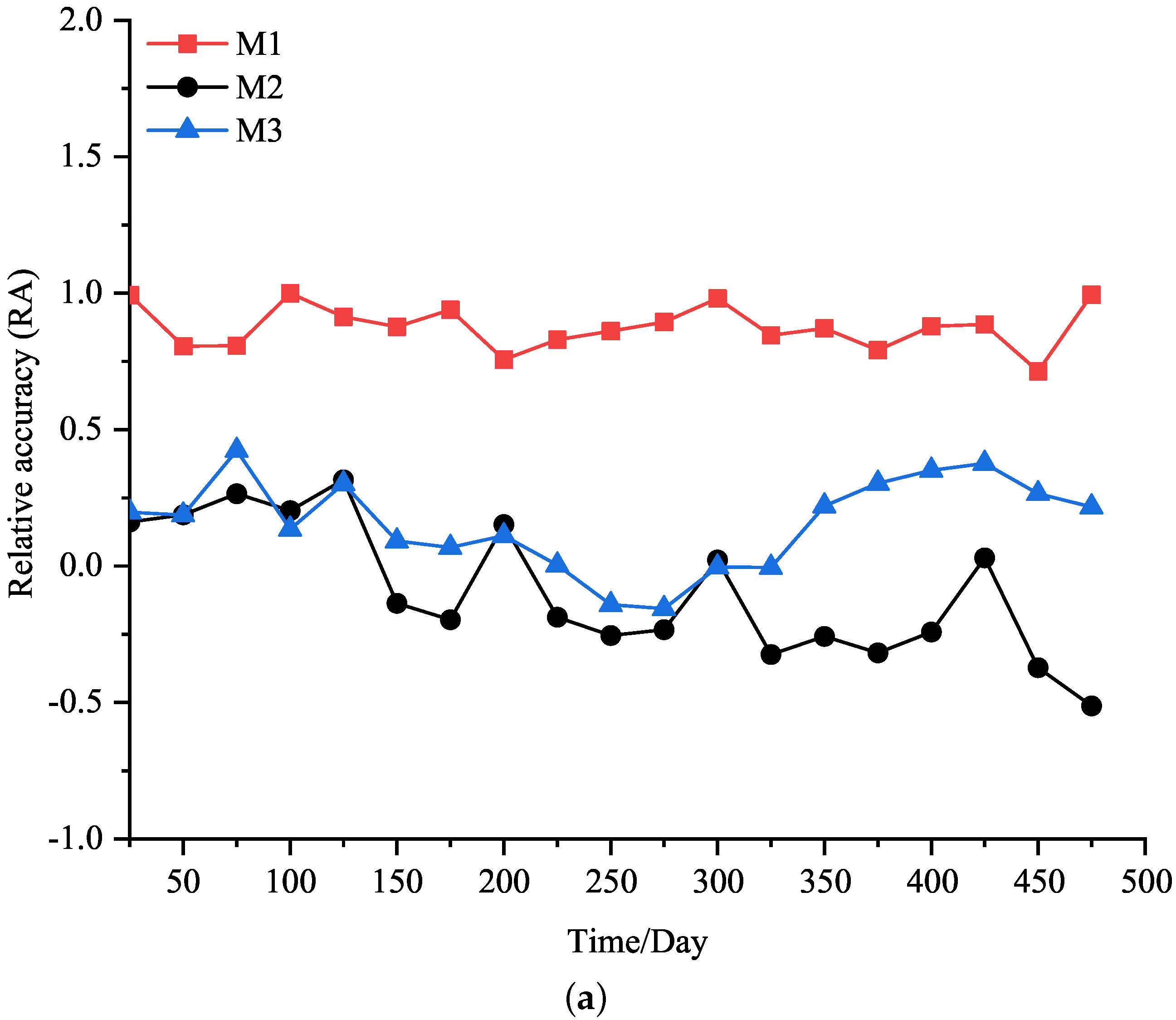
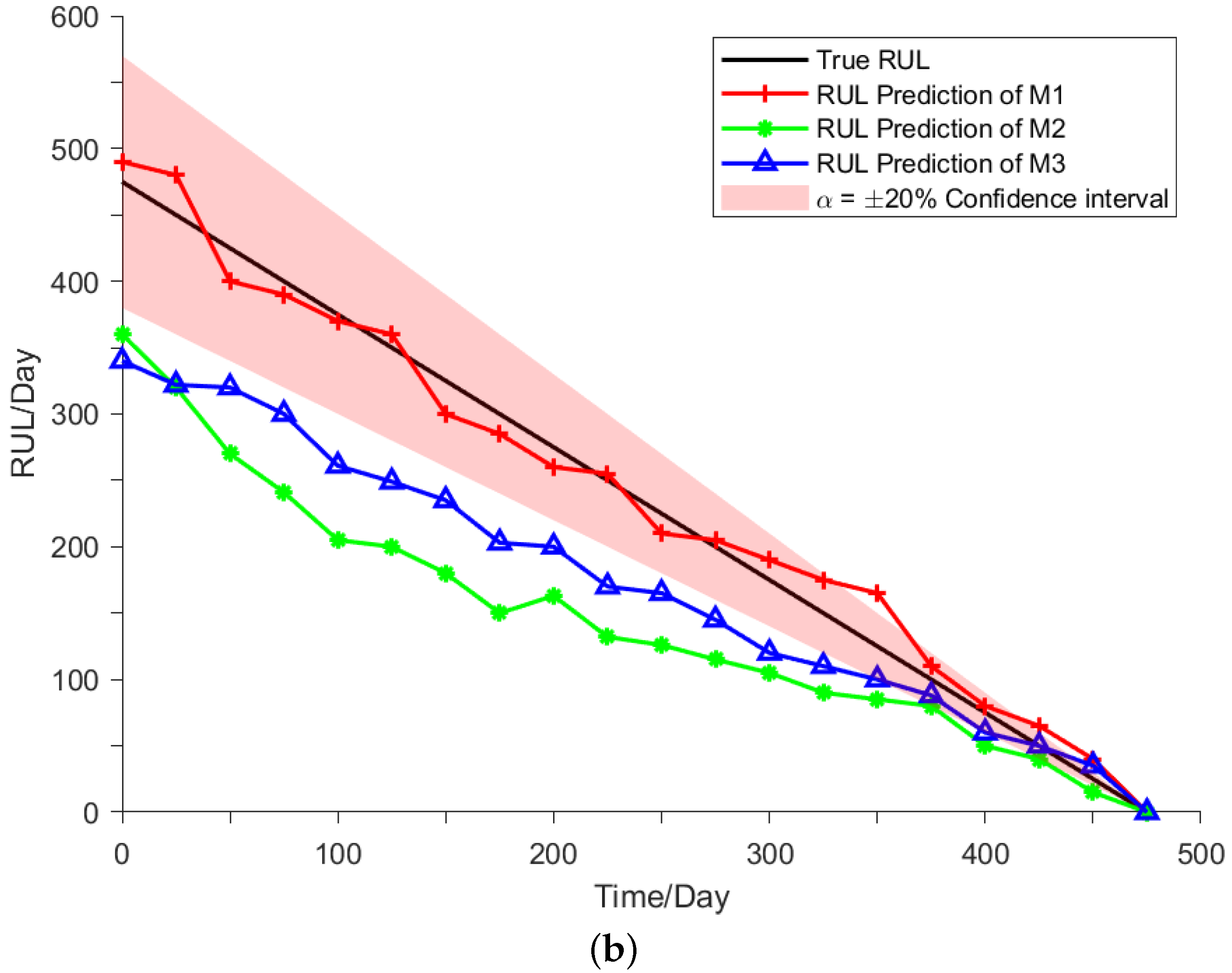
4.2. RUL Prediction

The method proposed in this paper is denoted as M1. The method proposed in [44] is denoted as M2. The method in [45] is denoted as M3. By comparing the prediction results of the three prediction methods, the accuracy of the prediction model proposed in this paper is proved. Taking the bearing data of the first group as historical data, it is brought into the degradation model of this article, and the results of parameter estimation are $\widehat{{\mu }_{\alpha ,0}}=0.189,\widehat{{\sigma }_{\alpha ,0}}=0.015,\widehat{\beta }=1.135,\widehat{\sigma }=0.9871$. Bring the parameter estimation results into Equation (9) to perform RUL prediction. The prediction degenerate path is shown in Figure 6.

It can be seen from Figure 6 that the degradation result predicted by M1 is closer to the true value, followed by M3, and M2 has the lowest accuracy. With the running time increases, the degree of deviation between the predicted signal of M2 and M3 and the original signal becomes more and more apparent. Further analysis shows that the larger predicted value of M2 is because it does not consider the influence of nonlinearity on the Wiener process, which leads to the more immense predicted value. M3 considers the non-linear Wiener process but does not adopt the real-time update strategy, and the parameter estimation value cannot be updated in real-time, making the predicted value larger. Both M2 and M3 are pessimistic estimates, which may cause delays in replacement time and reduce equipment reliability.

In order to further prove the superiority of this method, we introduced Mean Absolute Error (MAE) and Root Mean Square Error (RMSE) [55] to analyze the error between the predicted value and the true value of the three methods.

$$\mathrm{MAE}=\frac{1}{N}\sum _1^N|l_n^{*}-l_n|$$

(39)

$$\mathrm{RMSE}=\sqrt{\frac{1}{N}\sum _1^N{(l_n^{*}-l_n)}^2}$$

(40)

where, $l_n^{*}$ is the predicted value at the current moment, $l_n$ is the true value at the current moment, and N is the number of samples. The smaller the value of MAE and RMAE, the higher the accuracy.

Table 1. Bearing error under 3 methods.

Method	MAE	MAE Lift Rate	RMSE	RMSE Lift Rate
M1	0.240	-	0.378	-
M2	0.548	56.20%	0.703	46.23%
M3	0.485	50.52%	0.621	24.30%

shows the error between the predicted value of the three methods and the true value. The method M1 in this paper is minor than M2 and M3 in both MAE and RMSE. The values of MAE and RMSE of M2 are the lowest, followed by M3, which matches the prediction result of Figure 6. The MAE of M1 is 56.20% and 50.25% higher than M2 and M3. Compared with M2 and M3, the RMSE of M1 has increased by 46.23% and 24.30%, respectively. Therefore, the method presented in this paper has higher accuracy in the prediction of residual life. It is worth noting that M3 is lower than M2 in both MAE and RMSE, which indicates that the introduction of a non-linear Wiener process will make the prediction model more effective.

In order to further prove the accuracy of the method in this paper, we introduce the relative accuracy (RA) criterion [56].

$$\mathrm{RA}=1-|\frac{l_n^{*}-l_n}{l_n}|$$

(41)

The larger the RA, the higher the accuracy of the method. Figure 7 shows the accuracy analysis results of the three methods.

It can be seen from Figure 7a that the relative accuracy of M1 is greater than that of M2 and M3. It further shows that the M1 method proposed in this article is more accurate than M2 and M3, proving that the nonlinear Wiener degradation process is close to the actual degradation process of the equipment.

According to the literature [56], the confidence interval is 20%. It can be seen from Figure 7b that most of the remaining values predicted by M1 fall within the confidence interval of ±20% of the true life. The RUL predicted by M2 and M3 almost all fall outside the confidence interval, which further proves that the method in this paper can accurately predict the remaining life of the equipment.

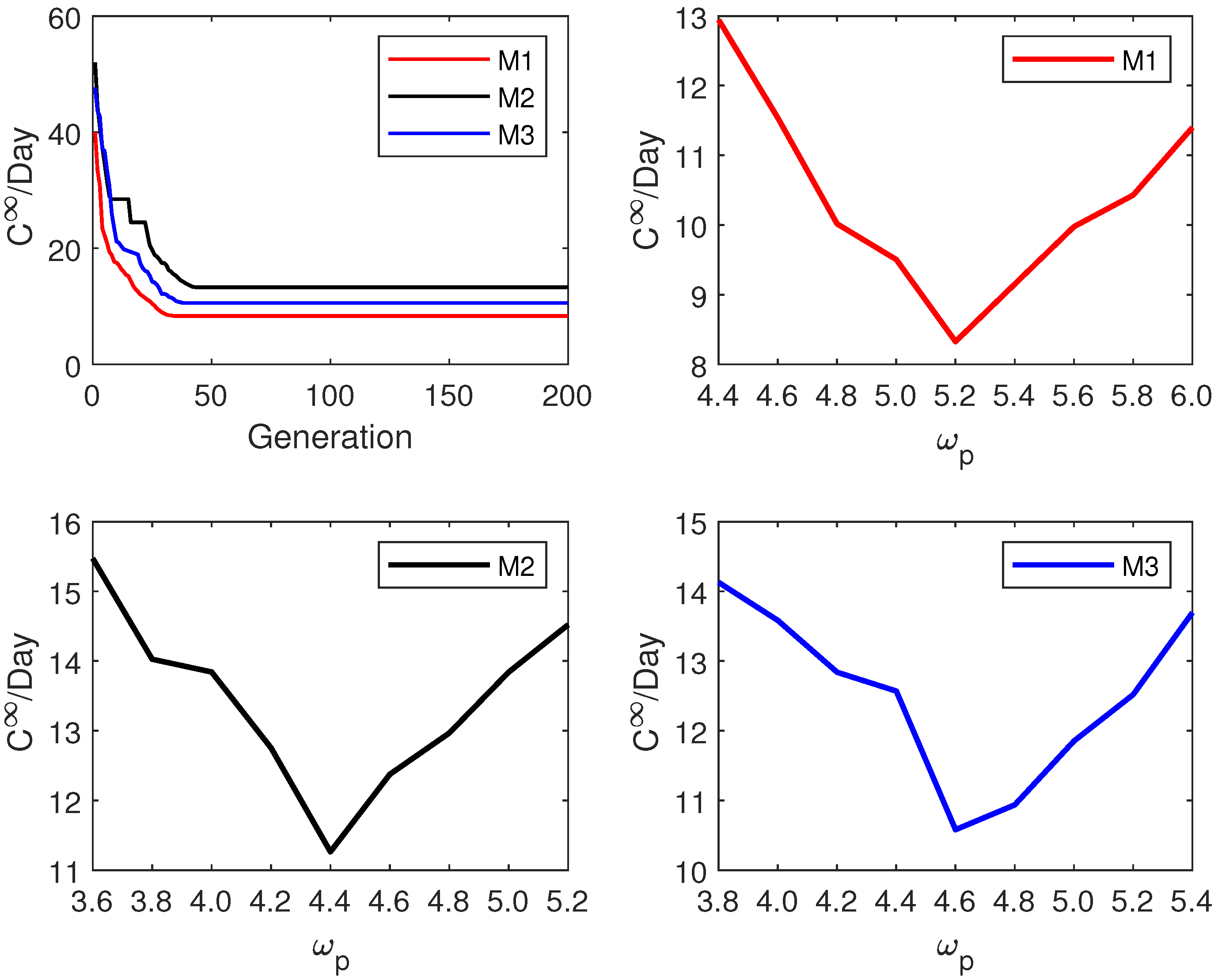
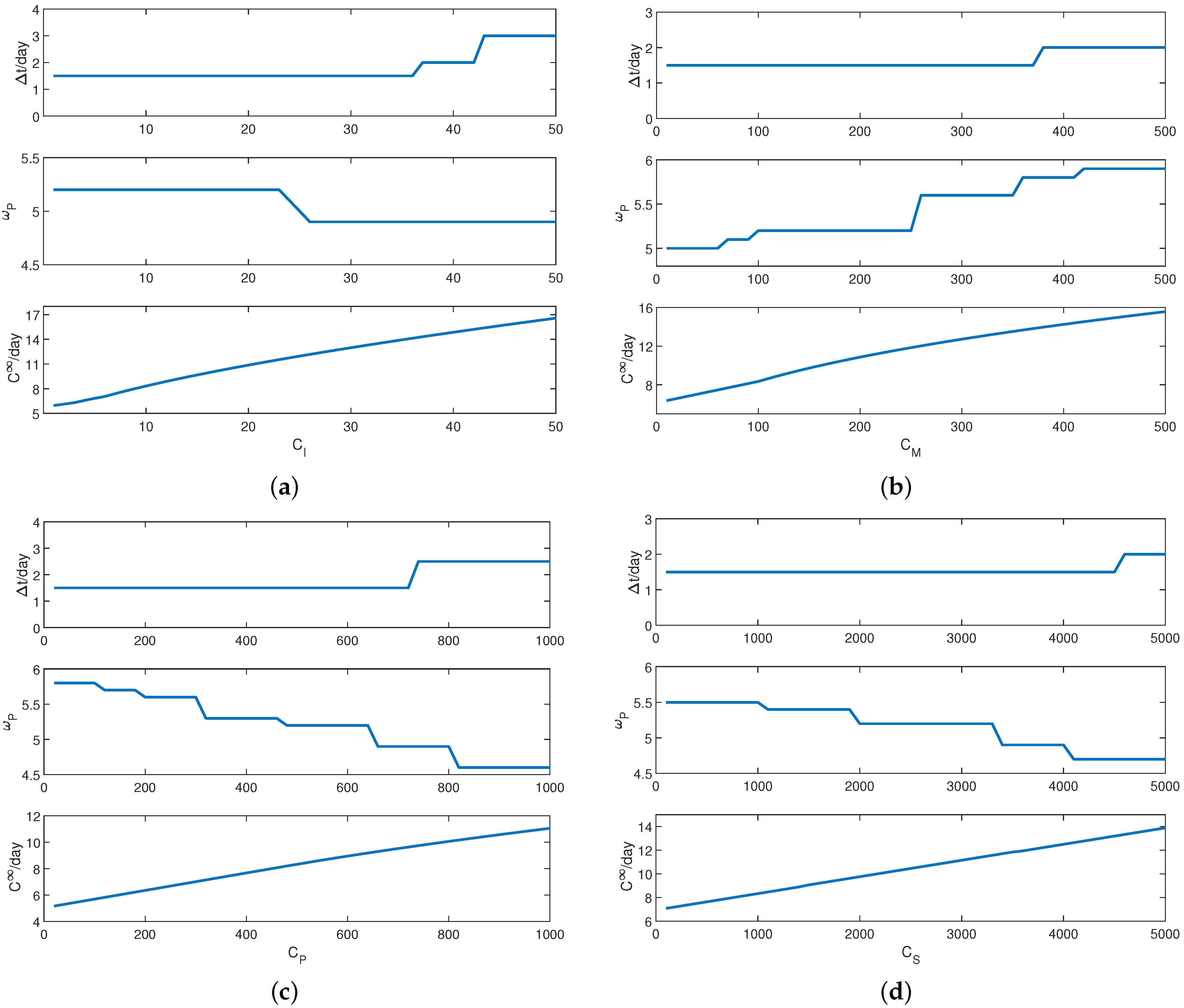
4.3. Decision Analysis

According to the information of the remaining life prediction, the maintenance activities are arranged. The specific costs of the maintenance activities are shown in

Table 2. Maintenance fee schedule.

Parameter	${\mathit{C}}_{\mathit{I}}$	${\mathit{C}}_{\mathit{M}}$	${\mathit{C}}_{\mathit{P}}$	${\mathit{C}}_{\mathit{S}}$
Cost/$	10	100	500	1000

.

Based on the above prediction information, the genetic algorithm is used to iterate the three models to solve the optimal long-term expense ratio. The iteration parameters are consistent. The number of iterations is 200. The iteration results are shown in Figure 8.

Figure 8 shows the process of solving the optimal average cost rate by two different methods. It can be seen from the figure that the long-term average cost rate of M1 is $8.33, the average cost rate solved by M2 is $13.26, and the average cost rate solved by M3 is $10.58. Compared with M2 and M3, the lowest average cost of M1 is reduced by 37.17% and 21.26%, respectively. When ${\omega }_p<5.2$ in the M1 solving process, the maintenance cost rate decreases monotonically with the increase of the maintenance threshold. When ${\omega }_p>5.2$, the maintenance cost rate increases monotonically with the increase of the maintenance threshold. When the preventive maintenance threshold ${\omega }_p=5.2$, there is a minimum average cost rate of $8.33. Similarly, when ${\omega }_p=4.4$ in M2, there is a minimum average expense rate of $13.26. When ${\omega }_p=4.6$ in M3, there is a minimum average expense rate of $10.58. It further illustrates that the method of this article can obtain better maintenance decision results. This is because the prediction results of M2 and M3 are conservative, which reduces the RUL value, increases the number of maintenance and maintenance costs. The prediction model of this article can accurately predict the RUL, reducing the loss caused by excessive maintenance.

4.4. Discussion

It can be seen from the above results that model in this paper dramatically improves the accuracy of equipment life prediction and makes the maintenance decision results more reasonable. The maintenance decision model established based on the RUL prediction information eliminates the disadvantages of traditional preventive maintenance, reduces maintenance costs, and improves maintenance efficiency. The following further discusses the sensitivity of maintenance cost parameters in the maintenance decision model proposed in this paper. Based on the controlled variable method, the single maintenance cost for each change, other costs and conditions remain unchanged. Therefore, we studied the changes in the maintenance strategy with the changes of various costs. Since $C_I<C_M<C_P<C_S$, let $C_I\in [1,50],C_M\in [1,500],C_P\in [1,1000],C_S\in [1,5000]$. The relationship between maintenance cost parameters and optimal maintenance strategy is shown in Figure 9.

Figure 9 a–d are the relationship between inspection costs $C_I$, preventive maintenance costs $C_M$, preventive replacement costs $C_P$, failure replacement costs $C_S$, and maintenance strategies, respectively. For the $C^{\infty }$, the lowest long-term expense ratio increases approximately linearly with various expenses. With $C_I$ from 1 to 50, the $C^{\infty }$ from 5.69/day to 16.58/day, with a growth rate of 0.22. The rate of increase in the $C^{\infty }$ caused by $C_M$, $C_P$ and $C_S$ was 0.018, 0.006 and 0.0014. It can be seen that the long-term average cost rate has the highest sensitivity to the inspection cost. This is because the inspection work is performed more frequently in the entire maintenance activity, and the inspection cost directly affects the total maintenance cost.

For the ${\omega }_p$, as $C_I$, $C_P$, and $C_S$ increase, ${\omega }_p$ decreases, and as $C_M$ increases, ${\omega }_p$ increases. The main reason for the increase in ${\omega }_p$ is that when $C_M$ is low, there is a lower ${\omega }_p$, which can increase the maintenance frequency to ensure the stable operation of the equipment, and $C_M$ continues to increase, a lower ${\omega }_p$ will generate many maintenance costs, so ${\omega }_p$ rises. $C_I$ has a low impact on the ${\omega }_p$, so ${\omega }_p$ does not change significantly with $C_I$. However, with the increase of $C_P$ and $C_S$, it is necessary to increase the preventive frequency to extend preventive replacement and failure replacement and reduce the total cost. Therefore, the ${\omega }_p$ decreases.

For the $\Delta t$, as the various costs increase, $\Delta t$ keeps increasing, and the total cost is reduced by increasing the $\Delta t$. The impact of the $C_I$ pair is the most significant because when the $C_I$ is low, the operation of the equipment can be learned in time through frequent inspections to ensure the reliable and safe operation of the equipment. When the $C_I$ increases, frequent inspections will inevitably lead to increased maintenance costs, so increase t to reduce costs. In summary, $C_I$ has the most significant impact on $C^{\infty }$ and $\Delta t$, $C_M$ has the most significant impact on ${\omega }_p$, and $C_P$ and $C_P$ have relatively low impacts on various indicators of the maintenance strategy. Therefore, the actual maintenance activities should focus on controlling $C_M$ and $C_M$ to reduce maintenance costs on the premise of ensuring the reliable operation of the equipment.

5. Conclusions

Based on the data-driven method, this paper established the RUL prediction and maintenance decision model of the deterioration equipment. We used the measured data to verify the model’s accuracy. The conclusions are as follows:

(1)

For stochastic deterioration equipment, the nonlinear Wiener process can represent the true degradation process of the device more accurately than the linear Wiener process, which conforms to objective laws and effectively improves the accuracy of RUL prediction.

(2)

The introduction of online parameter updates can improve the accuracy and reliability of RUL prediction.

(3)

Based on the more accurate RUL prediction results, a more realistic optimal maintenance strategy can be formulated, reducing maintenance costs and prolonging the RUL of the equipment.

(4)

Inspection costs and preventive maintenance costs have a significant impact on maintenance strategies. Therefore, it is necessary to focus on controlling inspection costs and preventive maintenance costs to promote sustainable development in actual maintenance activities.

References

- Iheukwumere-Esotu, L.O.; Yunusa-Kaltungo, A. Knowledge Criticality Assessment and Codification Framework for Major Maintenance Activities: A Case Study of Cement Rotary Kiln Plant. Sustainability 2021, 13, 4619. [Google Scholar] [CrossRef]
- Pei, H.; Hu, C.; Si, X.; Zhang, J.; Pang, Z.; Zhang, P. Summary of equipment remaining life prediction methods based on machine learning. Chin. J. Mech. Eng. 2019, 55, 1–13. [Google Scholar] [CrossRef] [Green Version]
- Tichy, T.; Broz, J.; Belinova, Z.; Pirnik, R. Analysis of Predictive Maintenance for Tunnel Systems. Sustainability 2021, 13, 3977. [Google Scholar] [CrossRef]
- Liu, H.; Jia, W.; Zhang, D.; Tan, J. The Research Status and Challenges of Deep Learning in the Technology of Predicting the Remaining Service Life of Equipment. Comput. Integr. Manuf. Syst. 2021, 27, 34–52. [Google Scholar]
- Sarute, U.; Hathaikarn, M. A critical review on cellulose: From fundamental to an approach on sensor technology. Renew. Sustain. Energy Rev. 2015, 41, 401–412. [Google Scholar]
- Park, S.; Hamm, S.Y.; Kim, J. Performance Evaluation of the GIS-Based Data-Mining Techniques Decision Tree, Random Forest, and Rotation Forest for Landslide Susceptibility Modeling. Sustainability 2019, 11, 5659. [Google Scholar] [CrossRef] [Green Version]
- Kamble, S.S.; Gunasekaran, A.; Ghadge, A.; Raut, R. A performance measurement system for industry 4.0 enabled smart manufacturing system in SMMEs—A review and empirical investigation. Int. J. Prod. Econ. 2020, 229, 107853. [Google Scholar] [CrossRef]
- Ammar, Y.; Alqahtani, S.M.; Gupta, K.N. Warranty and maintenance analysis of sensor embedded products using internet of things in industry 4.0. Int. J. Prod. Econ. 2019, 208, 483–499. [Google Scholar]
- Jafari, L.; Makis, V. Joint optimal lot sizing and preventive maintenance policy for a production facility subject to condition monitoring. Int. J. Prod. Econ. 2015, 169, 156–168. [Google Scholar] [CrossRef]
- Lin, Y.; Li, X.; Hu, Y. Deep diagnostics and prognostics: An integrated hierarchical learning framework in PHM applications. Appl. Soft. Comput. 2018, 72, 555–564. [Google Scholar] [CrossRef]
- Rodrigues, L.R.; Yoneyama, T. A spare parts inventory control model based on Prognostics and Health monitoring data under a fill rate constraint. Comput. Ind. Eng. 2020, 148, 106724. [Google Scholar] [CrossRef]
- Ma, J.; Shang, P.; Zou, X.; Ma, N.; Ding, Y.; Sun, J.; Cheng, Y.; Tao, L.; Lu, C.; Su, Y.; et al. A hybrid transfer learning scheme for remaining useful life prediction and cycle life test optimization of different formulation Li-ion power batteries. Appl. Energy. 2021, 282, 116167. [Google Scholar] [CrossRef]
- Dawn, A.; Nam, H.; Kim, J. Practical options for selecting data-driven or physics-based prognostics algorithms with reviews. Eng. Syst. Saf. 2015, 133, 223–236. [Google Scholar]
- Omer, F.; Eker, F.; Ian, K. Physics-based prognostic modelling of filter clogging phenomena. Mech. Syst. Signal Proc. 2016, 75, 395–412. [Google Scholar]
- Guo, J.; Li, Z.; Li, M. A Review on Prognostics Methods for Engineering Systems. IEEE Trans. Reliab. 2020, 69, 1110–1129. [Google Scholar] [CrossRef]
- Sun, H.; Cao, D.; Zhao, Z. A Hybrid Approach to Cutting Tool Remaining Useful Life Prediction Based on the Wiener Process. IEEE Trans. Reliab. 2018, 67, 1294–1303. [Google Scholar] [CrossRef]
- Wang, B.; Lei, Y.; Li, N. A Hybrid Prognostics Approach for Estimating Remaining Useful Life of Rolling Element Bearings. IEEE Trans. Reliab. 2020, 69, 401–412. [Google Scholar] [CrossRef]
- Feng, Y.; Mohamed, S.; Yan, S. Remaining useful life prediction of induction motors using nonlinear degradation of health index. Mech. Syst. Signal Proc. 2021, 148, 107183. [Google Scholar]
- Yang, X.; Fang, Z.; Li, X. Similarity-based information fusion grey model for remaining useful life prediction of aircraft engines. Grey Syst. Theory Appl. 2020. ahead-of-print. [Google Scholar] [CrossRef]
- Zheng, X.; Zhang, X.; Si, C.; Lei, T.G. Degradation data analysis and remaining useful life estimation: A review on Wiener-process-based methods. Eur. J. Oper. Res. 2018, 271, 775–796. [Google Scholar] [CrossRef]
- Akhilesh, K.; Ratna, B.C.; Finn, T. An HMM and polynomial regression based approach for remaining useful life and health state estimation of cutting tools. Comput. Ind. Eng. 2019, 128, 1008–1014. [Google Scholar]
- Mosayeb, E.; Grall, E.; Shemehsavar, S. A dynamic auto-adaptive predictive maintenance policy for degradation with unknown parameters. Eur. J. Oper. Res. 2020, 282, 81–92. [Google Scholar] [CrossRef] [Green Version]
- Van, T.; Hong, T.; Bo-Suk, Y.; Tan, T. Machine performance degradation assessment and remaining useful life prediction using proportional hazard model and support vector machine. Mech. Syst. Signal Proc. 2012, 32, 320–330. [Google Scholar]
- Han, C.; Kong, X.G.; Chen, G.; Wang, Q.B.; Wang, R.B. Transferable convolutional neural network based remaining useful life prediction of bearing under multiple failure behaviors. Measurement 2021, 168, 108286. [Google Scholar]
- Chen, Z.; Wu, M.; Zhao, R. Machine Remaining Useful Life Prediction via an Attention Based Deep Learning Approach. IEEE Trans. Ind. Electron. 2021, 68, 2521–2531. [Google Scholar] [CrossRef]
- Meng, M.; Zhu, M. Deep Convolution-based LSTM Network for Remaining Useful Life Prediction. IEEE Trans. Ind. Inform. 2021, 17, 1658–1667. [Google Scholar]
- Singpurwalla, N.D. Survival in Dynamic Environments. Stat. Sci. 1995, 10, 86–103. [Google Scholar] [CrossRef]
- Lorton, A.; Fouladirad, M.; Grall, A. A methodology for probabilistic model-based prognosis. Eur. J. Oper. Res. 2013, 225, 443–454. [Google Scholar] [CrossRef]
- Zhang, M.; Ye, Z.; Xie, M. A condition-based maintenance strategy for heterogeneous populations. Comput. Ind. Eng. 2014, 77, 103–114. [Google Scholar] [CrossRef]
- Kleijnen, J.P. Regression and Kriging metamodels with their experimental designs in simulation: A review. Eur. J. Oper. Res. 2017, 256, 1–16. [Google Scholar] [CrossRef] [Green Version]
- Feng, D.; Guan, J. Planning of step-stress accelerated degradation test based on non-stationary gamma process with random effects. Comput. Ind. Eng. 2020, 125, 467–479. [Google Scholar]
- Cao, Y.; Liu, S.; Fang, Z.; Dong, W. Modeling ageing effects in the context of continuous degradation and random shock. Comput. Ind. Eng. 2020, 145, 106539. [Google Scholar] [CrossRef]
- Li, F.; Li, H.; He, Y. Adaptive stochastic model predictive control of linear systems using Gaussian process regression. IET Contr. Theory Appl. 2020, 15, 683–693. [Google Scholar] [CrossRef]
- Davis, C.B.; Hans, C.M.; Santner, T.J. Prediction of non-stationary response functions using a Bayesian composite Gaussian process. Comput. Stat. Data Anal. 2021, 154, 107083. [Google Scholar] [CrossRef]
- He, D.; Liu, L.; Cao, M. A doubly accelerated degradation model based on the inverse Gaussian process and its objective Bayesian analysis. J. Stat. Comput. Simul. 2021, 91, 1485–1503. [Google Scholar] [CrossRef]
- Zhai, Q.; Ye, Z. RUL Prediction of Deteriorating Products Using an Adaptive Wiener Process Model. IEEE Trans. Ind. Inform. 2017, 13, 2911–2921. [Google Scholar] [CrossRef]
- Wen, Y.; Wu, J.; Das, D.; Tseng, T. Degradation modeling and RUL prediction using Wiener process subject to multiple change points and unit heterogeneity. Reliab. Eng. Syst. Saf. 2018, 176, 113–124. [Google Scholar] [CrossRef]
- Li, N.; Lei, Y.; Yan, T. A Wiener Process Model-based Method for Remaining Useful Life Prediction Considering Unit-to-Unit Variability. IEEE Trans. Ind. Electron. 2018, 66, 2092–2101. [Google Scholar] [CrossRef]
- Man, J.; Zhou, Q. Prediction of hard failures with stochastic degradation signals using Wiener process and proportional hazards model. Comput. Ind. Eng. 2018, 125, 480–489. [Google Scholar] [CrossRef]
- Wang, H.; Ma, X.; Zhao, Y. An improved Wiener process model with adaptive drift and diffusion for online remaining useful life prediction. Mech. Syst. Signal Proc. 2018, 125, 370–387. [Google Scholar] [CrossRef]
- Liu, D.; Wang, S. A degradation modeling and reliability estimation method based on Wiener process and evidential variable. Reliab. Eng. Syst. Saf. 2020, 202, 106957. [Google Scholar] [CrossRef]
- Zhang, M.; Gaudoin, O.; Xie, M. Degradation-based maintenance decision using stochastic filtering for systems under imperfect maintenance. Eur. J. Oper. Res. 2015, 245, 531–541. [Google Scholar] [CrossRef]
- Liu, B.; Xie, M.; Xu, Z.; Kuo, W. An imperfect maintenance policy for mission-oriented systems subject to degradation and external shocks. Comput. Ind. Eng. 2016, 102, 21–32. [Google Scholar] [CrossRef] [Green Version]
- Pei, H.; Hu, C.; Si, X.; Zhang, Z.; Du, D. Equipment maintenance decision-making model based on remaining life prediction information under imperfect maintenance. Acta Autom. Sin. 2018, 44, 719–729. [Google Scholar]
- Wang, Z.; Chen, Y.; Cai, Z.; Xiang, H.; Wang, L. Prediction of remaining life of imperfect maintenance equipment based on compound inhomogeneous Poisson process. Chin. J. Mech. Eng. 2020, 56, 14–23. [Google Scholar] [CrossRef] [Green Version]
- Chen, Y.; Wang, Z. Optimal Maintenance Decision Based on Remaining Useful Lifetime Prediction for the Equipment Subject to Imperfect Maintenance. IEEE Access 2020, 8, 6704–6716. [Google Scholar] [CrossRef]
- Tang, S.; Yu, C.; Xue, W.; Guo, X.; Si, X. Remaining Useful Life Prediction of Lithium-Ion Batteries Based on the Wiener Process with Measurement Error. Energies 2014, 7, 520–547. [Google Scholar] [CrossRef] [Green Version]
- Gebraeel, N.Z.; Lawley, M.A.; Li, R.; Ryan, J.K. Residual-life distributions from component degradation signals: A Bayesian approach. IIE Trans. 2005, 37, 534–557. [Google Scholar] [CrossRef]
- Lee, M.-L.T.; Whitmore, G.A. Threshold Regression for Survival Analysis: Modeling Event Times by a Stochastic Process Reaching a Boundary. Stat. Sci. 2006, 21, 501–513. [Google Scholar] [CrossRef] [Green Version]
- Grall, A.; Dieulle, L.; Berenguer, C. Continuous-time predictive-maintenance scheduling for a deteriorating system. IEEE Trans. Reliab. 2001, 51, 141–150. [Google Scholar] [CrossRef] [Green Version]
- Wang, Y.; Pham, H. A Multi-Objective Optimization of Imperfect Preventive Maintenance Policy for Dependent Competing Risk Systems With Hidden Failure. IEEE Trans. Reliab. 2011, 60, 770–781. [Google Scholar] [CrossRef]
- Hu, Y.; Liu, B.; Qin, Z. Recursive Extended Least Squares Parameter Estimation for Wiener Nonlinear Systems with Moving Average Noises. Circuits Syst. Signal Process. 2014, 32, 655–664. [Google Scholar] [CrossRef]
- Zio, E.; Peloni, G. Particle filtering prognostic estimation of the remaining useful life of nonlinear components. Reliab. Eng. Syst. Saf. 2011, 96, 403–409. [Google Scholar] [CrossRef]
- Patrick, N.; Rafael, G.; Kamal, M.; Emmanuel, R. An Experimental Platform for Bearings Accelerated Life Test. In Proceedings of the IEEE International Conference on Prognostics and Health Management, Denver, CO, USA, 18 June 2012. [Google Scholar]
- Saxena, A.; Celaya, J.; Saha, B. Metrics for offlineevaluation of prognostic performance. Int. J. Progn. Health Manag. 2010, 1, 2153–2648. [Google Scholar]
- Thompson, P.A. An MSE statistic for comparing forecast accuracy across series. Int. J. Forecast. 1990, 6, 219–227. [Google Scholar] [CrossRef]