
Optimal Scheduling of Hydro–Thermal–Wind–Photovoltaic Generation Using Lightning Attachment Procedure Optimizer


Abstract
:1. Introduction

| Reference | Method | Year | Test System | Main Consideration |
|---|---|---|---|---|
| [26] | ALO | 2016 | Test System 1, Test System 3, Test System 5 | Valve-point loading effect (VPE), transmission loss. |
| [5] | RCGA-RTVM | 2014 | Test System 1 | Valve-point loading effect of thermal units, power transmission loss. |
| [27] | HMOCA incorporated DE | 2011 | Test System 1 | Minimization of emission issues. |
| [19] | Multi-objective hybrid grey wolf optimizer | 2018 | Test System 2 | Minimization of operational costs and pollution emissions |
| [28] | Fast convergence real-coded genetic algorithm | 2018 | Test System 2 | The effect of valve-point loading of thermal generator and transmission loss is taken into consideration |
| [10] | IHS | 2018 | Test System 1 | Valve-point loading effect of thermal units, power transmission loss of the system. |
| [29] | Improved DE | 2014 | Test System 1 | Prohibited discharge zones (PDZs) of hydro units, valve-point loading effect, ramp rate limits of thermal generators, transmission losses. |
| [30] | CPSO | 2019 | Test System 1 | Valve-point loading effect, prohibited discharge zones (PDZs) of hydro units. |
| [31] | MOABC | 2014 | Test System 1 | Valve-point loading effect, power transmission losses. |
| [32] | NSGSA-CM | 2014 | Test System1 | Emission of hydrothermal system. |
| [8] | TLBO | 2013 | Test System 1 | Valve-point effect of thermal plants, prohibited discharge zones (PDZs) of the water reservoir of the hydro units. |
| [33] | A hybrid CSA and PSO | 2013 | Test System 1 | Economic emission, power transmission loss, valve-point effect. |
| [34] | EP | 2004 | Test System 1 | Valve-point loading effect. |
| [11] | MDNLPSO | 2015 | Test System 1 | Prohibited discharge zones (PDZs) of the water reservoir of the hydro units, valve-point loading effect, transmission losses. |
| [35] | RCGA-AFSA | 2014 | Test System 1 | Valve-point loading effect, transmission losses, prohibited discharge zones (PDZs), ramp rate limits. |
| [36] | TLPSOS | 2017 | Test System 1 | Valve-point loading effect. |
- The hydro–thermal generation scheduling problem is solved for small and large test systems.
- The renewable energy resources including the wind and PV generation systems are considered in the STHS problem.
- The economic issues are considered with cost reduction in the STHS problem.
- Application of efficient optimizer called LAPO to solve the STHS problem with renewable energy resources.
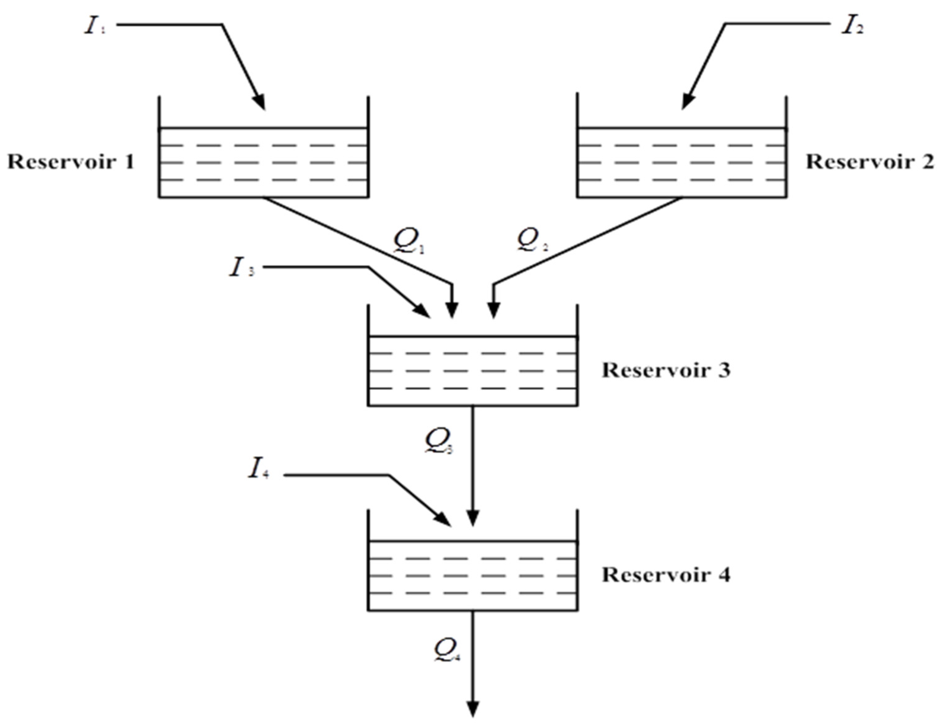
2. Problem Formulation of Hydrothermal Generation Scheduling with Wind and PV Power Integration System
2.1. The Cost Minimization
2.2. The Emission Rate Minimization
2.3. Constraints
2.4. Modeling of Wind and PV Power Generation
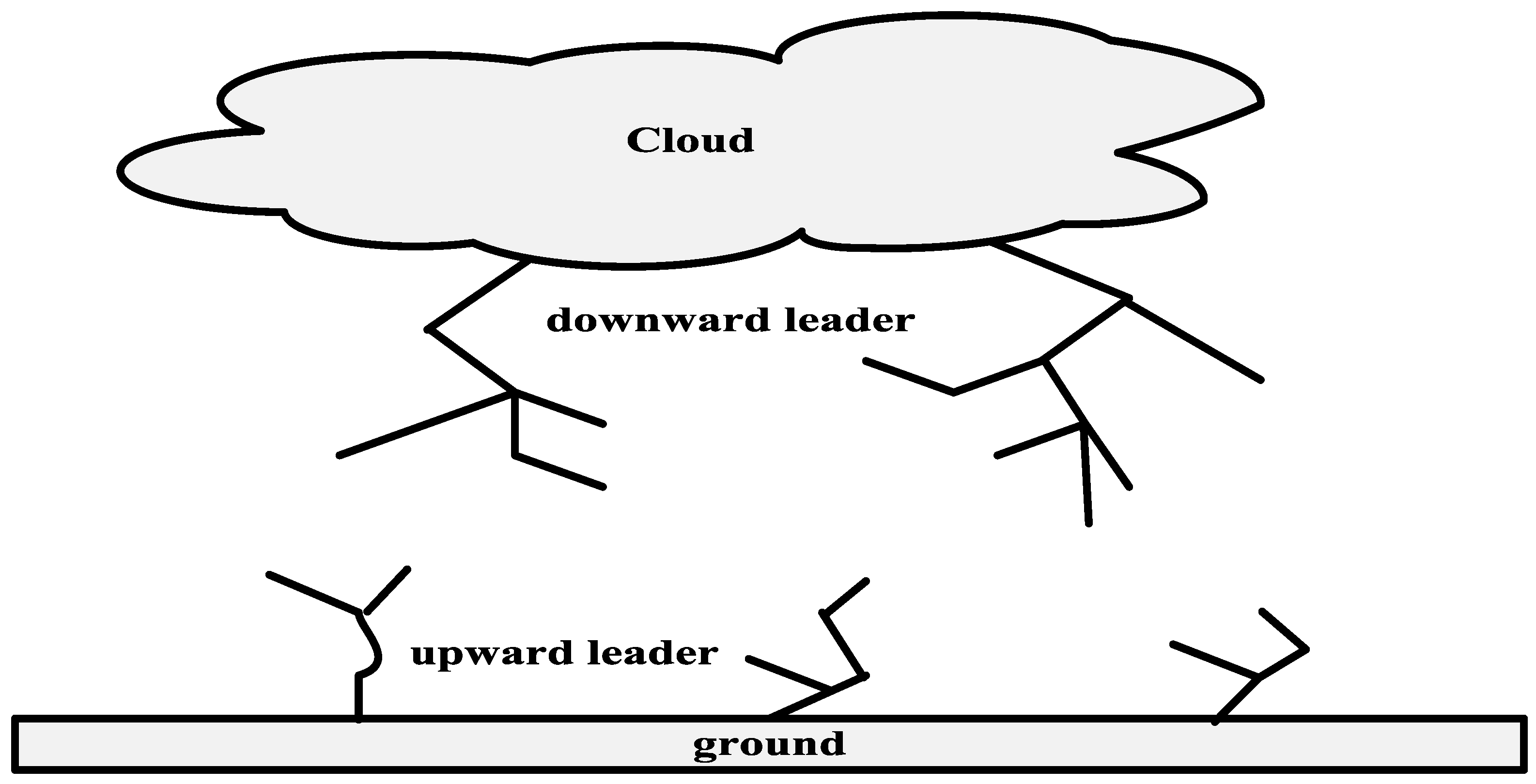
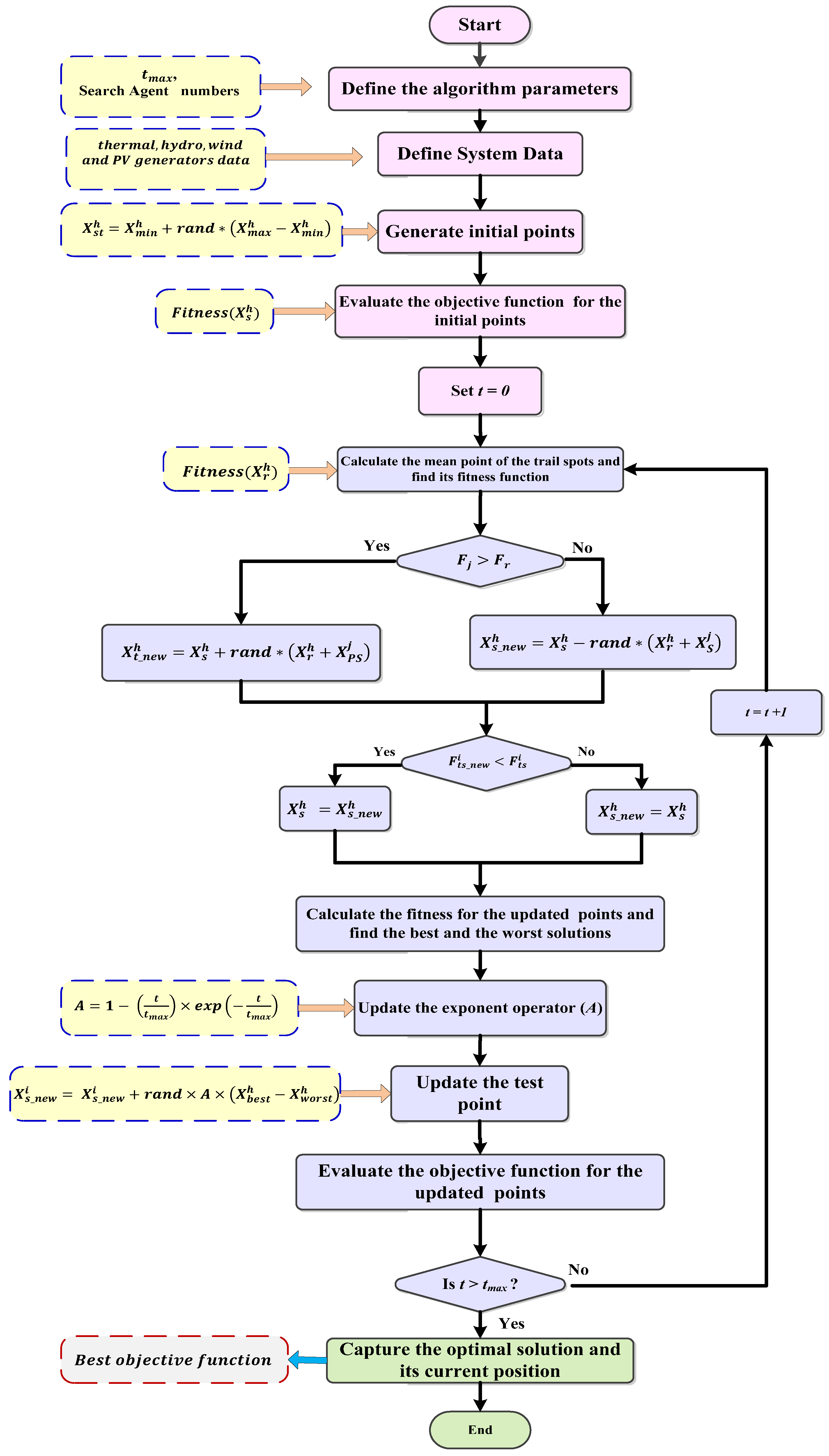
3. Lightning Attachment Procedure Optimization (LAPO)
Mathematical Model of LAPO
- Step 1: Trail spots
- Step 2: The next jumping of the initial points
- Step 3: Branch fading
- Step 4: Upward leader movement
- Step 5: The strike point
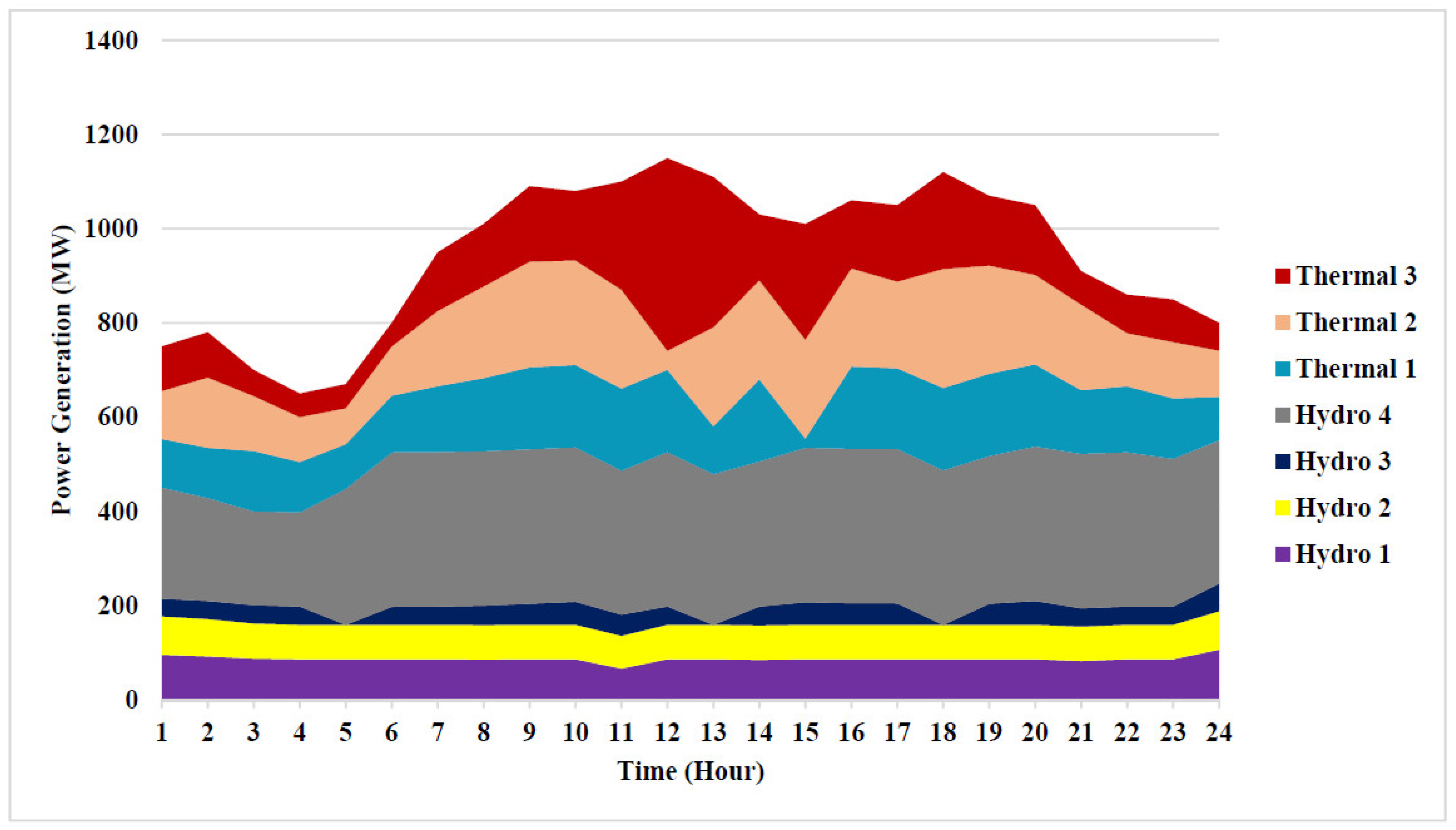
4. Simulation Results and Discussion
4.1. Test System 1
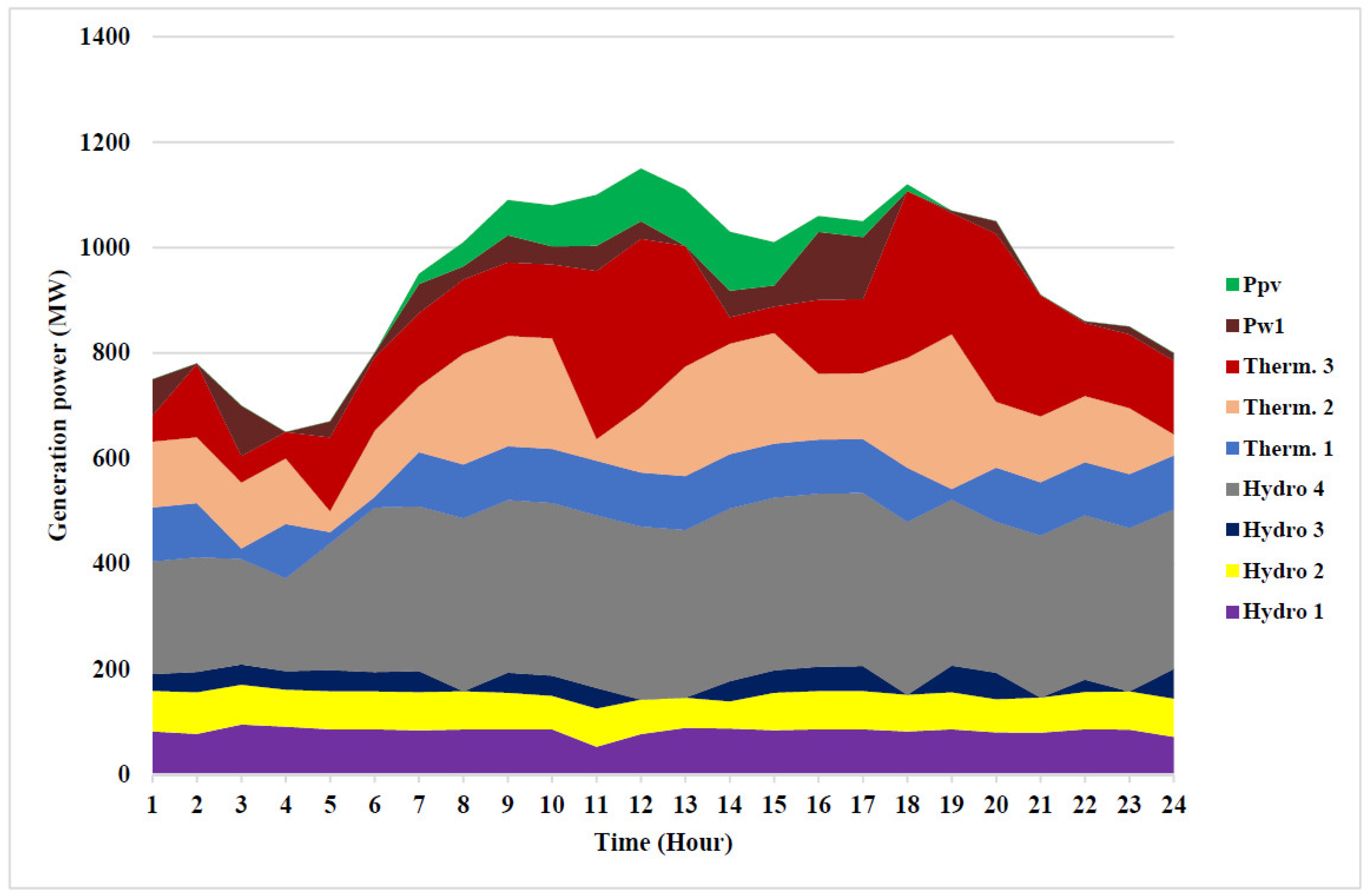
4.2. Test System 2
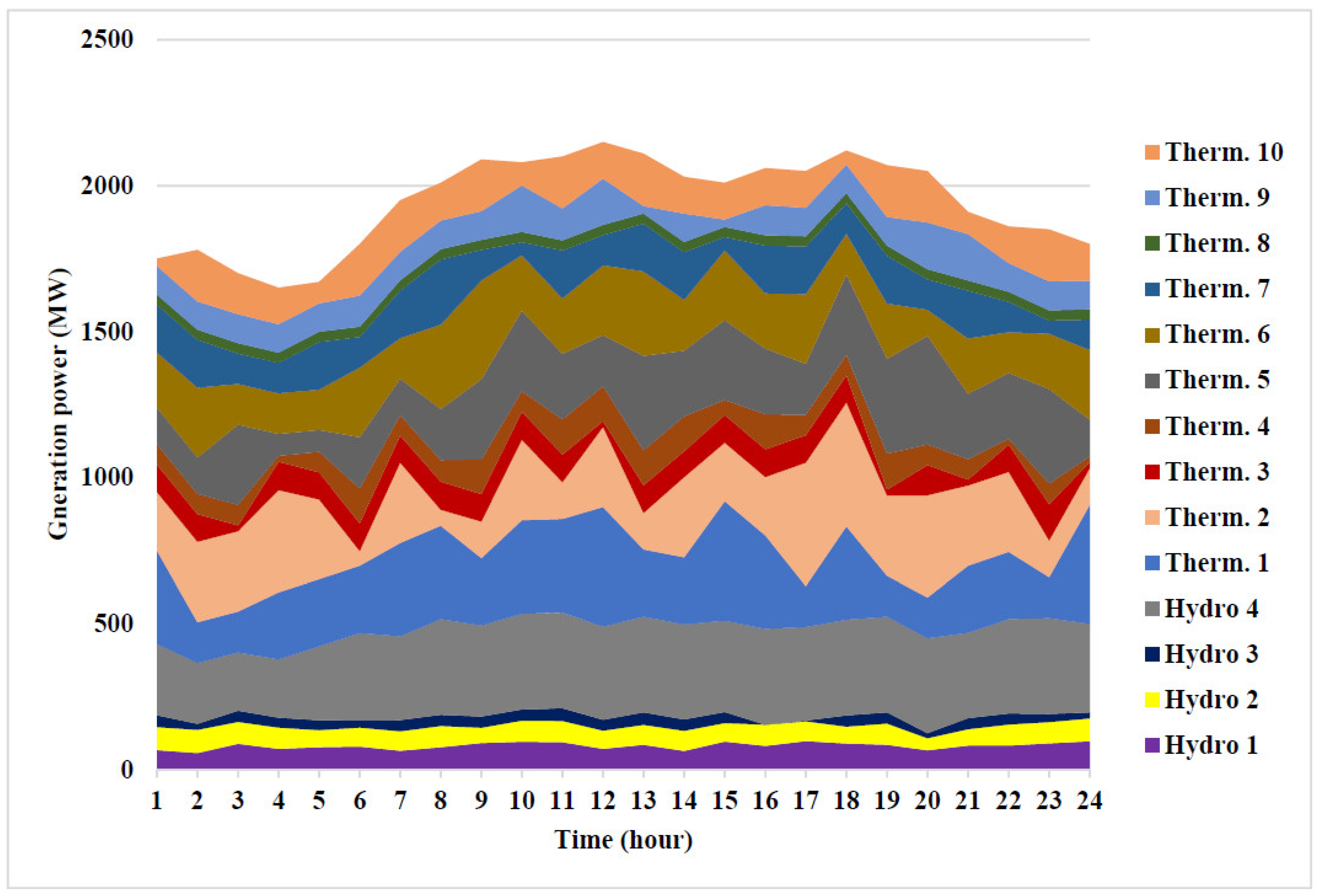
4.3. Test System 3
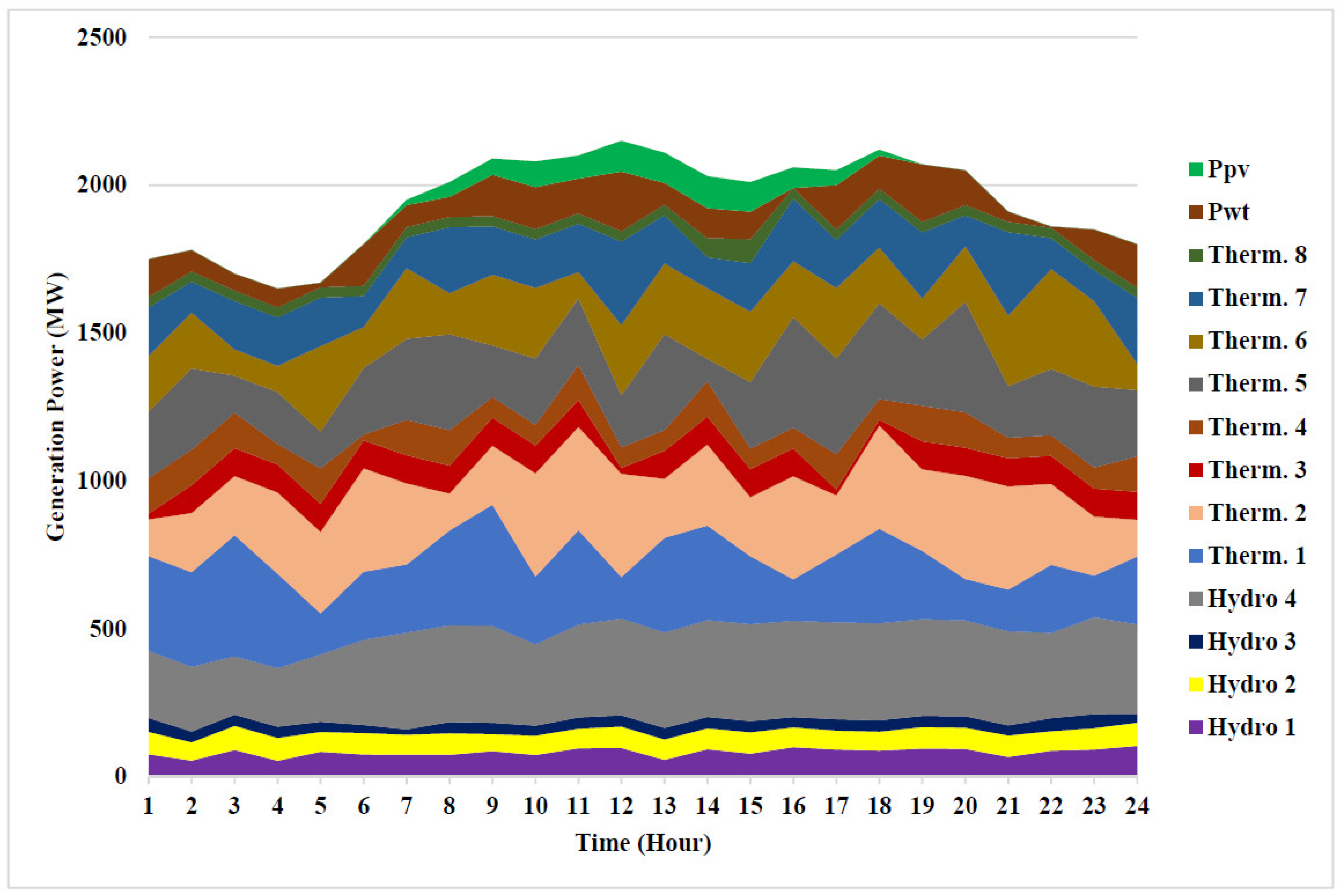
4.4. Test System 4
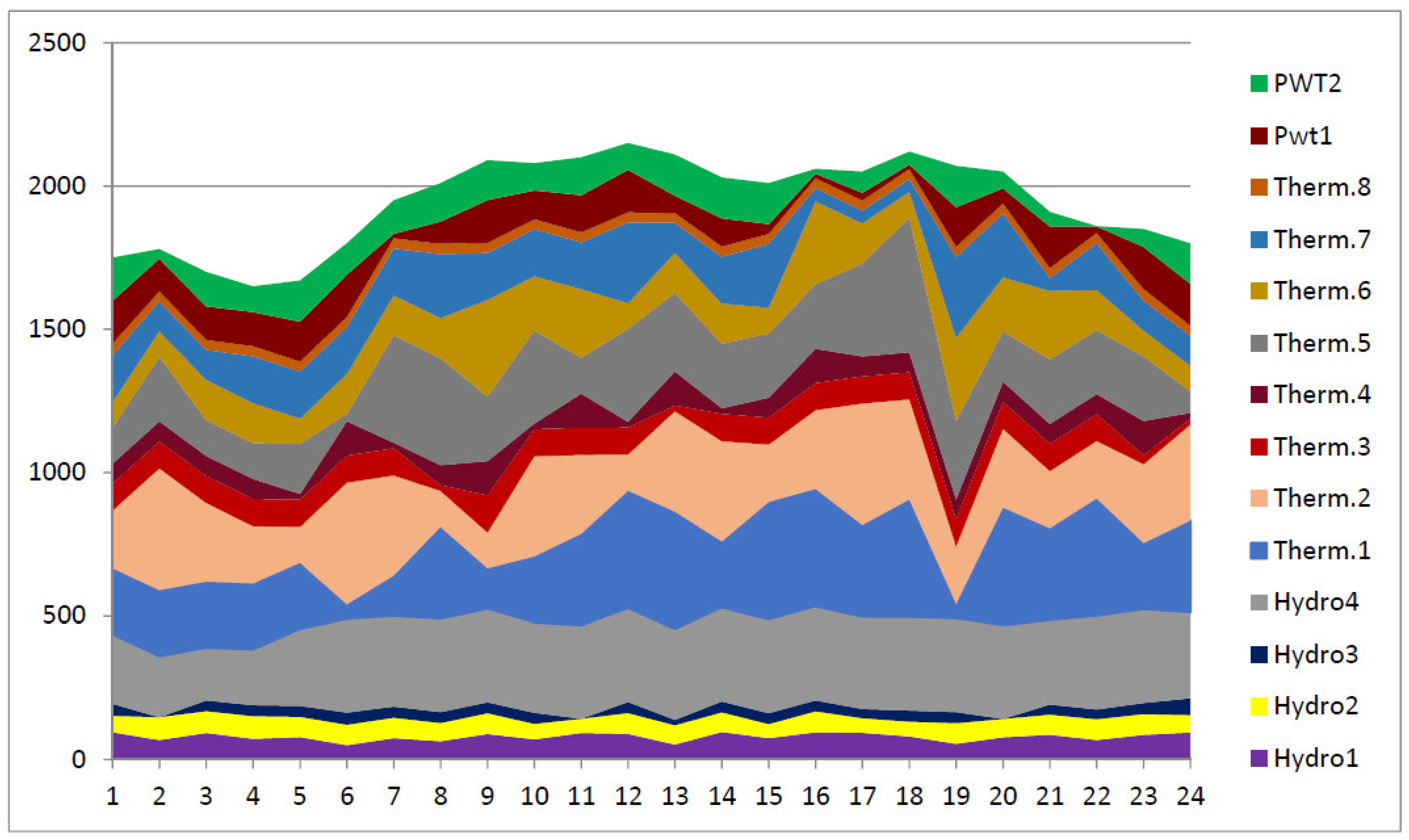
4.5. Test System 5
5. Conclusions
Author Contributions
Funding
Institutional Review Board Statement
Informed Consent Statement
Data Availability Statement
Conflicts of Interest
Nomenclature
| Total cost of thermal, wind, and PV-generating units | |
| Total cost of thermal-generating units | |
| Total cost of wind-generating units | |
| Total cost of PV-generating units. | |
| Total number of thermal-generating units | |
| Total number of wind-generating units | |
| Total number of PV-generating units | |
| T | length of total scheduling period |
| Power generation from thermal unit at time t | |
| Power generation from wind unit at time t | |
| Power generation from PV unit at time t | |
| ,, | Fuel cost coefficients of thermal unit |
| Minimum power generation limit of thermal unit | |
| , | Valve-point impact coefficients of thermal unit |
| Total amount of emission from all thermal units | |
| , , , , | Emission coefficients of the thermal units |
| Total number of hydropower-generating units | |
| Power load demand of the system at time t | |
| Power output of hydropower unit at time t | |
| Power losses of the hydrothermal system at time t | |
| , , , , | Power generation coefficients of hydropower unit |
| Reservoir storage volume of hydropower unit at time t | |
| Water discharge rate of hydropower unit at time t | |
| Power transmission loss of the system at time t | |
| Coefficients of power transmission loss | |
| External inflow to reservoir at time t | |
| Spillage discharge rate of reservoir at time t | |
| Number of upstream hydropower unit | |
| Minimum storage volume of hydropower unit | |
| Maximum storage volume of hydropower unit | |
| Minimum water discharge of hydropower unit | |
| Maximum water discharge of hydropower unit | |
| Minimum and maximum power generation of hydropower unit | |
| Minimum and maximum power generation of thermal unit | |
| Direct cost coefficient for wind power | |
| Rated power of wind-generating unit | |
| Cut in wind speed | |
| Cut out wind speed | |
| Rated wind speed | |
| Direct cost coefficient for PV power | |
| G | Forecast solar radiation |
| Solar radiation in the standard environment | |
| A certain radiation point | |
| Equivalent rated power output of the PV unit |
References
- Homem-de-Mello, T.; de Matos, V.L.; Finardi, E.C. Sampling strategies and stopping criteria for stochastic dual dynamic programming: A case study in long-term hydrothermal scheduling. Energy Syst. 2011, 2, 1–31. [Google Scholar] [CrossRef]
- Ahmadi, A.; Aghaei, J.; Shayanfar, H.A.; Rabiee, A. Mixed integer programming of multiobjective hydro-thermal self scheduling. Appl. Soft Comput. 2012, 12, 2137–2146. [Google Scholar] [CrossRef]
- Sawa, T.; Sato, Y.; Tsurugai, M.; Onishi, T. Daily integrated generation scheduling for thermal, pumped-storage, and cascaded hydro units and purchasing power considering network constraints. Electr. Eng. Jpn. 2011, 175, 25–34. [Google Scholar] [CrossRef]
- Dieu, V.N.; Ongsakul, W. Improved merit order and augmented Lagrange Hopfield network for short term hydrothermal scheduling. Energy Convers. Manag. 2009, 50, 3015–3023. [Google Scholar] [CrossRef]
- Haghrah, A.; Mohammadi-ivatloo, B.; Seyedmonir, S. Real coded genetic algorithm approach with random transfer vectors-based mutation for short-term hydro–thermal scheduling. IET Gener. Transm. Distrib. 2014, 9, 75–89. [Google Scholar] [CrossRef]
- Zhang, J.; Lin, S.; Qiu, W. A modified chaotic differential evolution algorithm for short-term optimal hydrothermal scheduling. Int. J. Electr. Power Energy Syst. 2015, 65, 159–168. [Google Scholar] [CrossRef]
- Mahor, A.; Rangnekar, S. Short term generation scheduling of cascaded hydro electric system using novel self adaptive inertia weight PSO. Int. J. Electr. Power Energy Syst. 2012, 34, 1–9. [Google Scholar] [CrossRef]
- Roy, P.K. Teaching learning based optimization for short-term hydrothermal scheduling problem considering valve point effect and prohibited discharge constraint. Int. J. Electr. Power Energy Syst. 2013, 53, 10–19. [Google Scholar] [CrossRef]
- Liao, X.; Zhou, J.; Ouyang, S.; Zhang, R.; Zhang, Y. An adaptive chaotic artificial bee colony algorithm for short-term hydrothermal generation scheduling. Int. J. Electr. Power Energy Syst. 2013, 53, 34–42. [Google Scholar] [CrossRef]
- Nazari-Heris, M.; Babaei, A.F.; Mohammadi-Ivatloo, B.; Asadi, S. Improved harmony search algorithm for the solution of non-linear non-convex short-term hydrothermal scheduling. Energy 2018, 151, 226–237. [Google Scholar] [CrossRef]
- Rasoulzadeh-Akhijahani, A.; Mohammadi-Ivatloo, B. Short-term hydrothermal generation scheduling by a modified dynamic neighborhood learning based particle swarm optimization. Int. J. Electr. Power Energy Syst. 2015, 67, 350–367. [Google Scholar] [CrossRef]
- Nazari-Heris, M.; Mohammadi-Ivatloo, B.; Haghrah, A. Optimal short-term generation scheduling of hydrothermal systems by implementation of real-coded genetic algorithm based on improved Mühlenbein mutation. Energy 2017, 128, 77–85. [Google Scholar] [CrossRef]
- Wang, Y.; Zhou, J.; Mo, L.; Zhang, R.; Zhang, Y. Short-term hydrothermal generation scheduling using differential real-coded quantum-inspired evolutionary algorithm. Energy 2012, 44, 657–671. [Google Scholar] [CrossRef]
- Zhang, H.; Yue, D.; Xie, X.; Dou, C.; Sun, F. Gradient decent based multi-objective cultural differential evolution for short-term hydrothermal optimal scheduling of economic emission with integrating wind power and photovoltaic power. Energy 2017, 122, 748–766. [Google Scholar] [CrossRef]
- Banerjee, S.; Dasgupta, K.; Chanda, C.K. Short term hydro–wind–thermal scheduling based on particle swarm optimization technique. Int. J. Electr. Power Energy Syst. 2016, 81, 275–288. [Google Scholar] [CrossRef]
- Dubey, H.M.; Pandit, M.; Panigrahi, B. Hydro-thermal-wind scheduling employing novel ant lion optimization technique with composite ranking index. Renew. Energy 2016, 99, 18–34. [Google Scholar] [CrossRef]
- Yuan, X.; Tian, H.; Yuan, Y.; Huang, Y.; Ikram, R.M. An extended NSGA-III for solution multi-objective hydro-thermal-wind scheduling considering wind power cost. Energy Convers. Manag. 2015, 96, 568–578. [Google Scholar] [CrossRef]
- Zhou, J.; Lu, P.; Li, Y.; Wang, C.; Yuan, L.; Mo, L. Short-term hydro-thermal-wind complementary scheduling considering uncertainty of wind power using an enhanced multi-objective bee colony optimization algorithm. Energy Convers. Manag. 2016, 123, 116–129. [Google Scholar] [CrossRef]
- Li, C.; Wang, W.; Chen, D. Multi-objective complementary scheduling of hydro-thermal-RE power system via a multi-objective hybrid grey wolf optimizer. Energy 2019, 171, 241–255. [Google Scholar] [CrossRef]
- Nematollahi, A.F.; Rahiminejad, A.; Vahidi, B. A novel physical based meta-heuristic optimization method known as lightning attachment procedure optimization. Appl. Soft Comput. 2017, 59, 596–621. [Google Scholar] [CrossRef]
- Nematollahi, A.F.; Rahiminejad, A.; Vahidi, B. A novel multi-objective optimization algorithm based on Lightning Attachment Procedure Optimization algorithm. Appl. Soft Comput. 2019, 75, 404–427. [Google Scholar] [CrossRef]
- Taher, M.A.; Kamel, S.; Jurado, F.; Ebeed, M. Optimal power flow solution incorporating a simplified UPFC model using lightning attachment procedure optimization. Int. Trans. Electr. Energy Syst. 2019, 30, 12170. [Google Scholar] [CrossRef]
- Youssef, H.; Kamel, S.; Ebeed, M. Optimal Power Flow Considering Loading Margin Stability Using Lightning Attachment Optimization Technique. In Proceedings of the 2018 Twentieth International Middle East Power Systems Conference (MEPCON), Cairo, Egypt, 18–20 December 2018; pp. 1053–1058. [Google Scholar]
- Hashemian, P.; Nematollahi, A.F.; Vahidi, B. A novel approach for optimal DG allocation in distribution network for minimizing voltage sag. Adv. Energy Res. 2019, 6, 55–73. [Google Scholar]
- Liu, W.; Yang, S.; Ye, Z.; Huang, Q.; Huang, Y. An Image Segmentation Method Based on Two-Dimensional Entropy and Chaotic Lightning Attachment Procedure Optimization Algorithm. Int. J. Pattern Recognit. Artif. Intell. 2017, 34, 2054030. [Google Scholar] [CrossRef]
- Dubey, H.M.; Pandit, M.; Panigrahi, B. Ant lion optimization for short-term wind integrated hydrothermal power generation scheduling. Int. J. Electr. Power Energy Syst. 2016, 83, 158–174. [Google Scholar] [CrossRef]
- Lu, S.; Sun, C. Quadratic approximation based differential evolution with valuable trade off approach for bi-objective short-term hydrothermal scheduling. Expert Syst. Appl. 2011, 38, 13950–13960. [Google Scholar] [CrossRef]
- Basu, M. Fast convergence real-coded genetic algorithm for short-term solar-wind-hydro-thermal generation scheduling. Electr. Power Compon. Syst. 2018, 46, 1239–1249. [Google Scholar] [CrossRef]
- Basu, M. Improved differential evolution for short-term hydrothermal scheduling. Int. J. Electr. Power Energy Syst. 2014, 58, 91–100. [Google Scholar] [CrossRef]
- Wu, Y.; Wu, Y.; Liu, X. Couple-based particle swarm optimization for short-term hydrothermal scheduling. Appl. Soft Comput. 2019, 74, 440–450. [Google Scholar] [CrossRef]
- Zhou, J.; Liao, X.; Ouyang, S.; Zhang, R.; Zhang, Y. Multi-objective artificial bee colony algorithm for short-term scheduling of hydrothermal system. Int. J. Electr. Power Energy Syst. 2014, 55, 542–553. [Google Scholar] [CrossRef]
- Tian, H.; Yuan, X.; Ji, B.; Chen, Z. Multi-objective optimization of short-term hydrothermal scheduling using non-dominated sorting gravitational search algorithm with chaotic mutation. Energy Convers. Manag. 2014, 81, 504–519. [Google Scholar] [CrossRef]
- Selvakumar, A.I. Civilized swarm optimization for multiobjective short-term hydrothermal scheduling. Int. J. Electr. Power Energy Syst. 2013, 51, 178–189. [Google Scholar] [CrossRef]
- Basu, M. An interactive fuzzy satisfying method based on evolutionary programming technique for multiobjective short-term hydrothermal scheduling. Electr. Power Syst. Res. 2004, 69, 277–285. [Google Scholar] [CrossRef]
- Fang, N.; Zhou, J.; Zhang, R.; Liu, Y.; Zhang, Y. A hybrid of real coded genetic algorithm and artificial fish swarm algorithm for short-term optimal hydrothermal scheduling. Int. J. Electr. Power Energy Syst. 2014, 62, 617–629. [Google Scholar] [CrossRef]
- Kang, C.; Guo, M.; Wang, J. Short-term hydrothermal scheduling using a two-stage linear programming with special ordered sets method. Water Resour. Manag. 2017, 31, 3329–3341. [Google Scholar] [CrossRef]
- Sun, C.; Lu, S. Short-term combined economic emission hydrothermal scheduling using improved quantum-behaved particle swarm optimization. Expert Syst. Appl. 2010, 37, 4232–4241. [Google Scholar] [CrossRef]
- Nazari-Heris, M.; Mohammadi-Ivatloo, B.; Gharehpetian, G. Short-term scheduling of hydro-based power plants considering application of heuristic algorithms: A comprehensive review. Renew. Sustain. Energy Rev. 2017, 74, 116–129. [Google Scholar] [CrossRef]
- Bhattacharjee, K.; Bhattacharya, A.; Dey, S.H.N. Real coded chemical reaction based optimization for short-term hydrothermal scheduling. Appl. Soft Comput. 2014, 24, 962–976. [Google Scholar] [CrossRef]
- James, J.; Li, V.O. A social spider algorithm for global optimization. Appl. Soft Comput. 2015, 30, 614–627. [Google Scholar]
- Swain, R.; Barisal, A.; Hota, P.; Chakrabarti, R. Short-term hydrothermal scheduling using clonal selection algorithm. Int. J. Electr. Power Energy Syst. 2011, 33, 647–656. [Google Scholar] [CrossRef]
- Lakshminarasimman, L.; Subramanian, S. Short-term scheduling of hydrothermal power system with cascaded reservoirs by using modified differential evolution. IEE Proc. Gener. Transm. Distrib. 2006, 153, 693–700. [Google Scholar] [CrossRef]
- Mandal, K.; Chakraborty, N. Differential evolution technique-based short-term economic generation scheduling of hydrothermal systems. Electr. Power Syst. Res. 2008, 78, 1972–1979. [Google Scholar] [CrossRef]
- Zhang, J.; Wang, J.; Yue, C. Small population-based particle swarm optimization for short-term hydrothermal scheduling. IEEE Trans. Power Syst. 2011, 27, 142–152. [Google Scholar] [CrossRef]


| Test System | Number of Hydrothermal Generation Units |
|---|---|
| Test System 1 | Four cascaded hydropower plants and three thermal plants |
| Test System 2 | Four cascaded hydropower plants, three thermal plants, and one equivalent wind-and-solar-generating unit |
| Test System 3 | Four hydro plants and ten thermal plants |
| Test System 4 | Four cascaded hydropower plants, eight thermal-power plants, and one equivalent wind- and equivalent solar-generating unit |
| Test System 5 | Four cascaded hydropower plants, eight thermal-power plants, and two wind-generating units |
| Hours (h) | Hydro Power (MW) | Thermal Power (MW) | Total Load (MW) | |||||||||
|---|---|---|---|---|---|---|---|---|---|---|---|---|
| Qh1 | Qh2 | Qh3 | Qh4 | Ph1 | Ph2 | Ph3 | Ph4 | Ps1 | Ps2 | Ps3 | PD | |
| 1 | 11.881 | 14.880 | 17.128 | 10.441 | 92.37 | 83.227 | 29.169 | 177.984 | 102.638 | 124.877 | 139.724 | 750 |
| 2 | 5.299 | 6.082 | 22.175 | 17.215 | 55.483 | 46.549 | 4.485 | 216.396 | 102.675 | 124.887 | 229.522 | 780 |
| 3 | 13.802 | 13.592 | 11.488 | 23.312 | 95.463 | 78.521 | 38.674 | 207.574 | 20.012 | 209.757 | 50.007 | 700 |
| 4 | 14.552 | 14.352 | 27.639 | 24.236 | 91.949 | 75.821 | 0 | 199.121 | 102.669 | 40.001 | 139.801 | 650 |
| 5 | 5.8224 | 14.9813 | 25.821 | 15.967 | 56.246 | 72.473 | 0 | 258.852 | 102.664 | 40.0032 | 139.766 | 670 |
| 6 | 14.999 | 13.753 | 10.080 | 24.148 | 87.053 | 70.288 | 38.070 | 325.225 | 99.596 | 40 | 139.778 | 800 |
| 7 | 14.061 | 14.363 | 22.972 | 24.989 | 86.437 | 71.486 | 0 | 327.820 | 20.148 | 124.834 | 319.271 | 950 |
| 8 | 13.674 | 8.094 | 29.754 | 24.582 | 86.147 | 48.528 | 0 | 326.620 | 20.004 | 209.427 | 319.263 | 1010 |
| 9 | 14.951 | 12.124 | 10.746 | 14.313 | 86.628 | 65.992 | 38.504 | 262.311 | 102.671 | 124.897 | 409.013 | 1090 |
| 10 | 12.068 | 14.793 | 22.851 | 16.660 | 83.597 | 72.197 | 0 | 282.772 | 102.626 | 40.000 | 498.795 | 1080 |
| 11 | 10.949 | 12.881 | 29.978 | 22.735 | 81.118 | 68.188 | 0 | 319.873 | 102.653 | 209.805 | 318.360 | 1100 |
| 12 | 12.959 | 14.548 | 12.827 | 23.469 | 85.279 | 71.807 | 43.305 | 322.807 | 102.587 | 294.706 | 229.505 | 1150 |
| 13 | 7.645 | 6.000 | 23.631 | 17.610 | 66.860 | 37.085 | 0 | 290.082 | 102.277 | 294.397 | 319.2940 | 1110 |
| 14 | 12.479 | 12.934 | 10.477 | 23.523 | 86.153 | 68.327 | 38.361 | 323.010 | 154.915 | 40.0035 | 319.270 | 1030 |
| 15 | 5.250 | 10.724 | 10.642 | 23.184 | 51.663 | 61.030 | 38.454 | 321.706 | 102.663 | 294.730 | 139.783 | 1010 |
| 16 | 14.999 | 14.999 | 14.427 | 24.872 | 89.021 | 72.499 | 36.103 | 313.277 | 20.000 | 209.811 | 319.274 | 1060 |
| 17 | 14.489 | 11.211 | 16.659 | 24.999 | 86.612 | 62.890 | 30.688 | 327.847 | 102.638 | 209.830 | 229.509 | 1050 |
| 18 | 14.999 | 14.990 | 10.003 | 20.425 | 86.620 | 72.486 | 38.052 | 308.464 | 174.906 | 209.925 | 229.517 | 1120 |
| 19 | 11.788 | 9.4846 | 28.025 | 24.983 | 82.931 | 55.652 | 0 | 327.803 | 164.339 | 209.750 | 229.523 | 1070 |
| 20 | 14.671 | 6.787 | 12.142 | 24.791 | 86.640 | 41.686 | 42.707 | 327.2481 | 102.671 | 40.000 | 409.035 | 1050 |
| 21 | 6.073 | 14.969 | 29.999 | 24.984 | 55.318 | 72.457 | 0 | 327.806 | 20.000 | 294.674 | 139.751 | 910 |
| 22 | 14.999 | 13.959 | 12.685 | 18.017 | 86.620 | 70.717 | 38.253 | 293.043 | 102.663 | 40.007 | 228.700 | 860 |
| 23 | 8.985 | 9.7949 | 10.115 | 22.697 | 72.635 | 57.085 | 38.099 | 319.711 | 102.658 | 209.802 | 50.007 | 850 |
| 24 | 10.875 | 14.999 | 16.860 | 24.925 | 95.751 | 80.948 | 54.837 | 303.378 | 174.997 | 40.096 | 50.000 | 800 |
| Algorithm | Minimum Cost ($) | Average Cost ($) | Maximum Cost ($) |
|---|---|---|---|
| LAPO | 38,800.75 | 38,915.23 | 39,520 |
| MDNLPSO [11] | 40,179 | 40,637 | 41,182 |
| CPSO [30] | 40,204.32 | 40,592.73 | 40,831.55 |
| TLPSOS [36] | 40,298.28 | 40,298.28 | 40,298.28 |
| ALO [26] | 40,780.05 | 41,094.3414 | 40,905.8259 |
| ORCCRO [39] | 40,936.65 | 41,127.6819 | 40,944.2938 |
| MCDE [6] | 40,945.75 | 41,380.54 | 41,977.04 |
| ACABC [9] | 41,074.42 | NA | NA |
| RCCRO [39] | 41,497.85 | 41,502.3669 | 41,498.2129 |
| DGSA [40] | 41,751.15 | 41,989.02 | 41,821.49 |
| CSA [41] | 42,244.057 | NA | NA |
| MDE [42] | 42,611.14 | NA | NA |
| PSO [43] | 44,740 | NA | NA |
| DE [42] | 44,526.10 | NA | NA |
| EP [34] | 45,063.004 | NA | NA |
| Hours (h) | Hydro Power (MW) | Thermal Power (MW) | RE (MW) | ||||||||||
|---|---|---|---|---|---|---|---|---|---|---|---|---|---|
| Qh1 | Qh2 | Qh3 | Qh4 | Ph1 | Ph2 | Ph3 | Ph4 | Ps1 | Ps2 | Ps3 | PW | PPV | |
| 1 | 9.214 | 11.549 | 17.709 | 14.811 | 82.387 | 76.720 | 32.173 | 213.054 | 102.571 | 124.750 | 50.023 | 68.322 | 0.000 |
| 2 | 8.346 | 13.687 | 11.911 | 18.839 | 77.682 | 78.995 | 38.624 | 216.981 | 102.667 | 125.000 | 139.579 | 0.471 | 0.000 |
| 3 | 14.193 | 13.851 | 12.169 | 24.678 | 95.500 | 75.487 | 38.541 | 199.442 | 20.039 | 124.891 | 50.611 | 95.489 | 0.000 |
| 4 | 14.220 | 12.885 | 14.895 | 16.886 | 91.504 | 69.912 | 35.216 | 176.028 | 102.677 | 124.414 | 50.187 | 0.062 | 0.000 |
| 5 | 13.870 | 14.851 | 10.651 | 16.432 | 86.411 | 72.285 | 40.201 | 239.963 | 21.040 | 40.048 | 139.760 | 30.292 | 0.000 |
| 6 | 14.899 | 14.466 | 14.094 | 20.989 | 86.636 | 71.666 | 36.656 | 311.552 | 20.139 | 125.324 | 139.808 | 8.219 | 0.000 |
| 7 | 12.497 | 14.848 | 12.257 | 21.012 | 84.489 | 72.280 | 40.319 | 311.675 | 102.908 | 124.833 | 139.044 | 55.117 | 19.335 |
| 8 | 13.760 | 14.968 | 27.689 | 24.915 | 86.222 | 72.455 | 0.000 | 327.607 | 101.950 | 209.887 | 141.301 | 24.918 | 45.660 |
| 9 | 14.102 | 13.266 | 12.985 | 24.794 | 86.461 | 69.171 | 38.014 | 327.257 | 102.080 | 209.225 | 139.617 | 51.327 | 66.849 |
| 10 | 14.698 | 11.287 | 12.181 | 24.731 | 86.642 | 63.165 | 38.536 | 327.070 | 102.492 | 209.928 | 139.937 | 34.530 | 77.700 |
| 11 | 5.568 | 14.985 | 11.813 | 24.755 | 53.512 | 72.479 | 38.646 | 327.140 | 103.595 | 40.865 | 319.245 | 47.760 | 96.758 |
| 12 | 9.268 | 11.928 | 24.017 | 24.962 | 77.378 | 65.369 | 0.000 | 327.743 | 102.440 | 124.195 | 319.332 | 33.382 | 100.160 |
| 13 | 13.923 | 9.859 | 24.269 | 22.203 | 89.011 | 57.372 | 0.000 | 317.535 | 102.291 | 208.071 | 228.475 | 0.699 | 106.545 |
| 14 | 14.015 | 8.542 | 13.182 | 24.768 | 87.832 | 51.307 | 38.563 | 327.178 | 102.924 | 209.795 | 50.003 | 50.578 | 111.820 |
| 15 | 12.347 | 14.105 | 14.311 | 24.698 | 84.717 | 71.007 | 42.464 | 326.969 | 102.577 | 210.031 | 50.059 | 40.255 | 81.921 |
| 16 | 14.169 | 14.878 | 12.355 | 24.979 | 86.496 | 72.325 | 46.364 | 327.792 | 102.600 | 124.843 | 140.478 | 128.744 | 30.358 |
| 17 | 14.169 | 14.878 | 12.355 | 24.979 | 86.496 | 72.325 | 47.449 | 327.792 | 102.600 | 124.843 | 140.478 | 117.659 | 30.358 |
| 18 | 11.599 | 13.383 | 29.762 | 24.953 | 82.442 | 69.451 | 0.000 | 327.717 | 102.436 | 208.437 | 316.964 | 0.000 | 12.578 |
| 19 | 14.358 | 13.659 | 10.378 | 23.671 | 86.575 | 70.083 | 50.714 | 314.179 | 20.040 | 293.928 | 229.887 | 4.596 | 0.000 |
| 20 | 10.979 | 11.158 | 14.787 | 17.918 | 80.634 | 62.695 | 50.447 | 285.915 | 102.682 | 124.674 | 318.791 | 24.162 | 0.000 |
| 21 | 10.802 | 12.270 | 29.105 | 22.065 | 80.059 | 66.442 | 0.000 | 306.975 | 101.140 | 124.853 | 230.298 | 0.233 | 0.000 |
| 22 | 14.492 | 13.813 | 18.592 | 20.909 | 86.613 | 70.416 | 23.588 | 311.124 | 101.058 | 125.484 | 138.634 | 3.084 | 0.000 |
| 23 | 13.513 | 14.921 | 28.134 | 22.546 | 85.989 | 72.388 | 0.000 | 309.510 | 102.278 | 125.034 | 139.843 | 14.959 | 0.000 |
| 24 | 7.005 | 11.643 | 10.194 | 24.448 | 72.180 | 72.364 | 56.414 | 302.196 | 102.296 | 40.040 | 139.651 | 14.859 | 0.000 |
| Total cost = $38,210.073 | |||||||||||||
| Hours (h) | Hydro Power (MW) | |||||||
|---|---|---|---|---|---|---|---|---|
| Qh1 | Qh2 | Qh3 | Qh4 | Ph1 | Ph2 | Ph3 | Ph4 | |
| 1 | 6.760 | 12.010 | 12.396 | 22.714 | 67.493 | 78.042 | 41.173 | 243.511 |
| 2 | 5.446 | 13.840 | 19.180 | 19.813 | 57.668 | 78.867 | 20.980 | 208.461 |
| 3 | 10.334 | 13.490 | 11.538 | 24.814 | 89.058 | 74.456 | 38.675 | 199.517 |
| 4 | 7.351 | 14.801 | 15.407 | 24.734 | 71.952 | 72.209 | 34.096 | 199.474 |
| 5 | 8.261 | 9.964 | 15.398 | 18.032 | 77.287 | 57.842 | 34.118 | 253.373 |
| 6 | 8.672 | 11.778 | 17.941 | 24.901 | 79.209 | 64.875 | 26.228 | 298.063 |
| 7 | 6.503 | 12.264 | 10.376 | 17.186 | 65.189 | 66.423 | 38.296 | 286.888 |
| 8 | 8.208 | 14.965 | 12.397 | 24.995 | 77.135 | 72.450 | 38.434 | 327.835 |
| 9 | 11.174 | 8.820 | 12.778 | 21.182 | 91.325 | 52.392 | 38.185 | 312.563 |
| 10 | 13.096 | 14.794 | 12.438 | 24.982 | 95.848 | 72.199 | 38.411 | 327.800 |
| 11 | 12.535 | 14.764 | 11.850 | 24.920 | 94.370 | 72.152 | 44.236 | 327.621 |
| 12 | 7.391 | 10.933 | 13.414 | 22.485 | 71.490 | 61.845 | 37.576 | 318.797 |
| 13 | 9.678 | 12.937 | 11.354 | 24.851 | 85.353 | 68.334 | 42.941 | 327.424 |
| 14 | 6.230 | 13.024 | 14.458 | 24.132 | 64.456 | 68.563 | 39.095 | 325.170 |
| 15 | 11.994 | 11.273 | 10.280 | 24.888 | 96.367 | 63.117 | 38.229 | 312.290 |
| 16 | 8.689 | 14.972 | 29.838 | 24.968 | 81.714 | 72.461 | 0.000 | 327.758 |
| 17 | 13.171 | 12.519 | 22.438 | 24.287 | 98.328 | 67.179 | 2.786 | 320.525 |
| 18 | 10.784 | 9.906 | 12.669 | 24.989 | 89.995 | 57.582 | 38.265 | 327.789 |
| 19 | 10.022 | 14.670 | 11.550 | 24.924 | 85.627 | 72.005 | 38.674 | 327.634 |
| 20 | 6.862 | 6.643 | 19.986 | 23.930 | 66.834 | 40.874 | 17.696 | 324.478 |
| 21 | 9.640 | 9.382 | 10.295 | 17.871 | 82.517 | 55.943 | 38.240 | 291.995 |
| 22 | 9.895 | 14.454 | 12.722 | 23.527 | 82.935 | 71.647 | 38.227 | 323.023 |
| 23 | 12.989 | 14.809 | 17.387 | 24.938 | 90.712 | 72.221 | 28.280 | 327.675 |
| 24 | 11.357 | 13.412 | 24.417 | 24.699 | 97.803 | 77.733 | 20.806 | 302.835 |
| Hours (h) | Thermal Power (MW) | |||||||||
|---|---|---|---|---|---|---|---|---|---|---|
| Ps1 | Ps2 | Ps3 | Ps4 | Ps5 | Ps6 | Ps7 | Ps8 | Ps9 | Ps10 | |
| 1 | 319.329 | 199.965 | 94.364 | 69.818 | 124.796 | 189.692 | 163.440 | 35.028 | 97.976 | 25.372 |
| 2 | 139.517 | 274.234 | 94.918 | 69.222 | 124.509 | 239.416 | 163.417 | 35.178 | 97.002 | 176.611 |
| 3 | 139.796 | 274.419 | 20.186 | 70.102 | 274.449 | 139.641 | 104.040 | 35.776 | 99.753 | 140.134 |
| 4 | 229.711 | 348.804 | 97.751 | 20.379 | 74.830 | 139.648 | 103.858 | 35.280 | 97.494 | 124.515 |
| 5 | 229.529 | 272.246 | 93.673 | 69.654 | 74.655 | 138.513 | 163.450 | 35.160 | 96.971 | 73.529 |
| 6 | 229.672 | 50.164 | 94.925 | 119.624 | 174.692 | 239.511 | 104.444 | 35.055 | 106.832 | 176.706 |
| 7 | 319.227 | 274.170 | 93.270 | 69.887 | 124.561 | 139.562 | 162.999 | 35.113 | 98.052 | 176.350 |
| 8 | 319.290 | 54.043 | 96.594 | 74.199 | 174.471 | 289.433 | 223.111 | 35.412 | 98.156 | 129.437 |
| 9 | 229.428 | 124.793 | 94.384 | 119.194 | 274.256 | 339.054 | 103.626 | 35.125 | 98.252 | 177.423 |
| 10 | 319.774 | 274.655 | 96.785 | 69.947 | 275.943 | 189.591 | 45.030 | 35.188 | 159.733 | 79.095 |
| 11 | 320.048 | 125.074 | 95.298 | 120.330 | 224.733 | 190.024 | 163.817 | 35.057 | 109.062 | 178.176 |
| 12 | 409.140 | 274.323 | 20.044 | 119.761 | 174.385 | 239.579 | 103.397 | 35.210 | 158.384 | 126.070 |
| 13 | 229.535 | 124.644 | 95.479 | 119.631 | 323.491 | 289.222 | 163.452 | 35.028 | 25.489 | 179.978 |
| 14 | 229.384 | 274.084 | 89.611 | 119.352 | 224.457 | 174.504 | 163.176 | 35.168 | 97.131 | 125.850 |
| 15 | 409.015 | 199.616 | 95.678 | 51.038 | 273.530 | 239.439 | 45.090 | 35.136 | 25.152 | 126.305 |
| 16 | 319.914 | 199.477 | 95.586 | 119.724 | 224.602 | 189.559 | 163.545 | 35.197 | 103.567 | 126.894 |
| 17 | 139.667 | 421.838 | 94.528 | 69.850 | 174.330 | 239.204 | 163.314 | 35.054 | 97.669 | 125.727 |
| 18 | 318.913 | 424.026 | 94.116 | 69.549 | 274.606 | 139.759 | 104.756 | 35.200 | 98.136 | 47.307 |
| 19 | 139.699 | 274.526 | 20.807 | 122.996 | 324.556 | 189.534 | 163.479 | 35.001 | 98.366 | 177.097 |
| 20 | 139.766 | 349.273 | 103.877 | 69.888 | 372.111 | 89.593 | 104.221 | 35.029 | 160.000 | 176.360 |
| 21 | 229.409 | 274.535 | 20.314 | 69.546 | 224.309 | 189.571 | 163.589 | 35.073 | 159.362 | 75.598 |
| 22 | 229.553 | 273.538 | 94.161 | 20.283 | 224.512 | 139.818 | 103.896 | 35.057 | 97.956 | 125.394 |
| 23 | 139.979 | 124.657 | 125.709 | 69.682 | 323.970 | 189.614 | 45.162 | 35.250 | 99.308 | 177.770 |
| 24 | 408.281 | 124.712 | 20.438 | 20.042 | 124.704 | 239.473 | 104.203 | 35.046 | 97.895 | 125.940 |
| Algorithm | Minimum Cost ($) | Average Cost ($) | Maximum Cost ($) |
|---|---|---|---|
| LAPO | 161,746.4 | 160,445.4 | 161,935.4 |
| ORCCRO [39] | 163,066.0337 | 163,068.7739 | 163,134.5391 |
| RCCRO [39] | 164,138.6517 | 164,140.3997 | 164,182.3520 |
| SPPSO [44] | 167,710.56 | 168,688.92 | 170,879.30 |
| SPSO [44] | 189,350.63 | 190,560.31 | 191,844.28 |
| MDE [44] | 177,338.60 | 179,676.35 | 182,172.01 |
| DE [44] | 170,964.15 | NA | NA |
| MCDE [6] | 165,331.7 | 166,116.4 | 167,060.6 |
| IDE [29] | 170,576.5 | 170,589.6 | 170,608.3 |
| Hours (h) | Hydro Power (MW) | |||||||
|---|---|---|---|---|---|---|---|---|
| Qh1 | Qh2 | Qh3 | Qh4 | Ph1 | Ph2 | Ph3 | Ph4 | |
| 1 | 7.925 | 11.136 | 15.490 | 17.354 | 75.249 | 75.421 | 47.159 | 227.490 |
| 2 | 5.078 | 8.343 | 14.311 | 21.083 | 54.305 | 61.768 | 36.305 | 219.114 |
| 3 | 10.601 | 14.585 | 12.904 | 23.173 | 89.848 | 80.999 | 38.084 | 197.853 |
| 4 | 5.035 | 14.937 | 10.163 | 23.248 | 53.819 | 76.729 | 38.139 | 197.966 |
| 5 | 9.371 | 12.213 | 14.935 | 20.424 | 83.602 | 66.927 | 35.134 | 227.198 |
| 6 | 7.893 | 14.849 | 17.662 | 18.952 | 74.767 | 72.282 | 27.285 | 288.448 |
| 7 | 7.700 | 12.670 | 19.807 | 24.977 | 73.598 | 67.610 | 17.971 | 327.784 |
| 8 | 7.617 | 14.965 | 12.444 | 24.949 | 73.424 | 72.450 | 38.407 | 327.706 |
| 9 | 9.724 | 9.908 | 11.767 | 24.971 | 85.735 | 57.592 | 38.654 | 327.768 |
| 10 | 7.420 | 11.803 | 15.315 | 15.756 | 73.029 | 64.957 | 34.309 | 275.292 |
| 11 | 11.805 | 12.253 | 13.303 | 21.505 | 95.566 | 66.390 | 37.699 | 314.207 |
| 12 | 12.573 | 14.425 | 10.641 | 24.884 | 96.840 | 71.595 | 38.454 | 327.518 |
| 13 | 5.281 | 13.149 | 10.977 | 23.574 | 56.699 | 68.882 | 38.593 | 323.198 |
| 14 | 10.655 | 13.712 | 11.106 | 24.824 | 92.592 | 70.199 | 38.628 | 327.344 |
| 15 | 7.839 | 14.589 | 12.495 | 24.839 | 77.490 | 71.875 | 38.378 | 327.389 |
| 16 | 12.480 | 12.249 | 14.955 | 24.290 | 99.433 | 66.379 | 35.094 | 325.690 |
| 17 | 10.413 | 11.508 | 10.692 | 24.870 | 91.299 | 63.953 | 38.479 | 327.478 |
| 18 | 9.809 | 11.459 | 12.541 | 24.985 | 87.891 | 63.780 | 38.350 | 327.809 |
| 19 | 11.788 | 14.915 | 12.980 | 24.958 | 94.466 | 72.379 | 38.018 | 327.731 |
| 20 | 12.334 | 14.378 | 11.587 | 23.847 | 93.418 | 71.513 | 38.825 | 324.188 |
| 21 | 6.813 | 14.810 | 15.299 | 22.369 | 66.486 | 72.223 | 34.345 | 318.285 |
| 22 | 10.775 | 12.098 | 13.103 | 17.363 | 87.322 | 65.910 | 44.132 | 288.231 |
| 23 | 12.974 | 14.599 | 12.428 | 24.829 | 91.633 | 71.891 | 47.674 | 327.360 |
| 24 | 13.248 | 13.390 | 22.845 | 24.330 | 103.979 | 77.677 | 30.710 | 301.884 |
| Hours (h) | Thermal Power (MW) | RE (MW) | ||||||||
|---|---|---|---|---|---|---|---|---|---|---|
| Ps1 | Ps2 | Ps3 | Ps4 | Ps5 | Ps6 | Ps7 | Ps8 | PW | PPV | |
| 1 | 318.954 | 124.729 | 20.295 | 119.772 | 224.470 | 189.373 | 163.447 | 35.046 | 128.594 | 0.000 |
| 2 | 319.204 | 199.490 | 94.699 | 119.729 | 274.595 | 189.569 | 104.305 | 35.018 | 71.901 | 0.000 |
| 3 | 409.050 | 199.469 | 94.804 | 119.806 | 124.718 | 89.731 | 163.589 | 35.039 | 57.009 | 0.000 |
| 4 | 318.863 | 274.326 | 94.814 | 69.773 | 174.555 | 89.699 | 163.398 | 35.030 | 62.889 | 0.000 |
| 5 | 139.716 | 274.361 | 94.885 | 119.779 | 124.720 | 289.084 | 163.466 | 35.030 | 16.097 | 0.000 |
| 6 | 229.527 | 349.173 | 94.792 | 20.002 | 224.382 | 139.288 | 104.094 | 35.211 | 140.749 | 0.000 |
| 7 | 229.463 | 274.415 | 94.673 | 119.744 | 274.411 | 239.455 | 104.165 | 35.050 | 74.084 | 17.578 |
| 8 | 319.457 | 124.946 | 94.690 | 119.736 | 324.078 | 139.814 | 222.600 | 35.001 | 68.185 | 49.506 |
| 9 | 408.844 | 199.612 | 94.827 | 69.784 | 174.546 | 239.541 | 163.433 | 35.007 | 139.598 | 55.060 |
| 10 | 227.804 | 349.206 | 94.654 | 69.714 | 224.281 | 239.431 | 163.565 | 35.096 | 141.773 | 86.892 |
| 11 | 319.096 | 348.906 | 91.073 | 119.106 | 224.369 | 89.717 | 163.312 | 35.053 | 117.605 | 77.900 |
| 12 | 139.747 | 348.787 | 20.258 | 69.993 | 174.635 | 239.439 | 281.758 | 35.280 | 201.329 | 104.366 |
| 13 | 319.311 | 199.617 | 94.858 | 70.001 | 324.266 | 239.510 | 163.518 | 35.198 | 73.874 | 102.474 |
| 14 | 319.276 | 273.995 | 94.863 | 119.828 | 74.873 | 239.589 | 104.270 | 65.497 | 100.768 | 108.276 |
| 15 | 229.371 | 199.615 | 94.800 | 69.740 | 224.442 | 239.345 | 163.326 | 81.612 | 92.618 | 100.000 |
| 16 | 139.556 | 348.993 | 94.357 | 69.838 | 374.046 | 189.469 | 211.563 | 35.222 | 0.359 | 70.000 |
| 17 | 229.473 | 199.584 | 20.049 | 119.624 | 323.928 | 238.441 | 162.997 | 35.007 | 149.688 | 50.000 |
| 18 | 319.281 | 349.163 | 20.012 | 69.952 | 323.873 | 189.469 | 163.467 | 35.010 | 111.943 | 20.000 |
| 19 | 229.989 | 275.560 | 94.824 | 119.889 | 224.421 | 139.663 | 222.982 | 35.115 | 194.962 | 0.000 |
| 20 | 139.536 | 349.005 | 94.735 | 119.753 | 373.954 | 188.513 | 104.283 | 35.036 | 117.229 | 0.000 |
| 21 | 139.913 | 349.328 | 94.877 | 69.823 | 174.495 | 239.085 | 281.896 | 35.002 | 34.240 | 0.000 |
| 22 | 229.447 | 274.283 | 94.236 | 69.878 | 224.328 | 338.203 | 104.277 | 35.295 | 4.457 | 0.000 |
| 23 | 140.274 | 199.654 | 94.907 | 70.537 | 274.360 | 289.342 | 104.221 | 35.010 | 103.137 | 0.000 |
| 24 | 229.062 | 124.378 | 94.552 | 119.675 | 224.191 | 89.683 | 222.729 | 35.001 | 146.479 | 0.000 |
| Total cost = $158,572.8 | ||||||||||
| Hours (h) | Hydro Power (MW) | |||||||
|---|---|---|---|---|---|---|---|---|
| Qh1 | Qh2 | Qh3 | Qh4 | Ph1 | Ph2 | Ph3 | Ph4 | |
| 1 | 13.316 | 7.132 | 11.064 | 22.027 | 95.066 | 57.177 | 41.893 | 242.550 |
| 2 | 7.040 | 12.185 | 28.964 | 24.946 | 68.327 | 79.129 | 0.000 | 213.308 |
| 3 | 12.744 | 11.740 | 13.309 | 18.662 | 92.605 | 75.627 | 37.694 | 184.675 |
| 4 | 7.893 | 14.223 | 11.299 | 21.508 | 72.162 | 78.542 | 38.663 | 194.459 |
| 5 | 9.245 | 12.197 | 13.519 | 24.784 | 78.394 | 69.949 | 38.921 | 268.703 |
| 6 | 5.009 | 13.766 | 12.985 | 24.913 | 50.562 | 70.315 | 42.524 | 327.603 |
| 7 | 8.443 | 14.087 | 11.702 | 24.675 | 74.779 | 70.971 | 38.663 | 316.807 |
| 8 | 6.605 | 11.315 | 10.069 | 24.565 | 63.751 | 63.267 | 38.061 | 326.566 |
| 9 | 11.825 | 14.696 | 10.162 | 24.809 | 89.352 | 72.046 | 38.138 | 326.801 |
| 10 | 7.516 | 9.069 | 12.159 | 24.439 | 70.567 | 53.646 | 38.545 | 315.488 |
| 11 | 12.529 | 8.077 | 27.485 | 24.431 | 92.583 | 49.146 | 0.000 | 326.146 |
| 12 | 11.663 | 14.945 | 11.957 | 24.967 | 89.493 | 72.422 | 38.612 | 327.758 |
| 13 | 5.014 | 12.388 | 19.548 | 22.084 | 52.444 | 66.798 | 19.242 | 316.991 |
| 14 | 14.496 | 12.684 | 10.880 | 24.986 | 96.493 | 67.650 | 38.560 | 327.810 |
| 15 | 7.929 | 8.042 | 10.029 | 24.885 | 74.595 | 48.980 | 38.026 | 327.522 |
| 16 | 13.486 | 14.917 | 11.407 | 24.948 | 95.129 | 72.381 | 38.672 | 327.704 |
| 17 | 13.720 | 8.489 | 15.930 | 23.143 | 93.003 | 50.665 | 32.787 | 321.546 |
| 18 | 9.791 | 8.562 | 11.804 | 24.508 | 80.948 | 51.054 | 38.647 | 326.388 |
| 19 | 5.540 | 14.547 | 11.370 | 24.852 | 54.812 | 71.805 | 38.670 | 327.425 |
| 20 | 9.321 | 11.304 | 27.960 | 24.982 | 77.946 | 63.228 | 0.000 | 327.798 |
| 21 | 14.980 | 13.563 | 14.761 | 18.274 | 86.624 | 69.868 | 35.484 | 294.858 |
| 22 | 8.133 | 14.743 | 15.343 | 24.659 | 68.189 | 72.121 | 34.245 | 326.854 |
| 23 | 13.571 | 14.905 | 12.201 | 24.985 | 86.048 | 72.364 | 38.527 | 327.807 |
| 24 | 10.661 | 8.840 | 13.440 | 23.732 | 94.775 | 60.017 | 58.977 | 300.161 |
| Hours (h) | Thermal Power (MW) | RE (MW) | ||||||||
|---|---|---|---|---|---|---|---|---|---|---|
| Ps1 | Ps2 | Ps3 | Ps4 | Ps5 | Ps6 | Ps7 | Ps8 | Pw1 | Pw2 | |
| 1 | 229.470 | 200.541 | 94.834 | 69.932 | 124.742 | 89.819 | 163.333 | 40.792 | 149.957 | 149.893 |
| 2 | 229.372 | 424.056 | 94.811 | 69.837 | 224.497 | 89.886 | 104.258 | 35.106 | 114.686 | 32.727 |
| 3 | 229.408 | 274.023 | 94.608 | 69.772 | 125.020 | 140.117 | 104.394 | 35.091 | 117.125 | 119.842 |
| 4 | 229.556 | 199.458 | 94.795 | 70.084 | 124.289 | 139.960 | 163.541 | 35.001 | 120.003 | 89.516 |
| 5 | 229.573 | 124.768 | 94.967 | 20.454 | 174.602 | 89.435 | 163.262 | 35.319 | 138.316 | 143.336 |
| 6 | 50.013 | 423.522 | 94.707 | 119.846 | 25.694 | 139.591 | 163.490 | 35.107 | 148.381 | 108.650 |
| 7 | 139.689 | 348.771 | 94.750 | 20.077 | 373.974 | 139.828 | 163.447 | 35.406 | 16.111 | 116.728 |
| 8 | 319.273 | 124.802 | 20.187 | 69.665 | 373.877 | 139.759 | 222.815 | 35.842 | 78.357 | 133.777 |
| 9 | 139.862 | 124.489 | 129.846 | 119.580 | 224.469 | 338.231 | 163.540 | 35.338 | 149.816 | 138.490 |
| 10 | 229.500 | 348.828 | 94.542 | 20.257 | 324.220 | 189.585 | 163.835 | 35.098 | 100.698 | 95.192 |
| 11 | 319.215 | 274.427 | 94.590 | 119.622 | 124.736 | 239.498 | 163.479 | 35.000 | 129.460 | 132.100 |
| 12 | 408.940 | 125.014 | 94.794 | 20.024 | 324.234 | 89.837 | 282.152 | 35.000 | 148.813 | 92.900 |
| 13 | 409.009 | 349.392 | 20.119 | 119.363 | 273.819 | 139.680 | 104.233 | 35.161 | 60.566 | 143.185 |
| 14 | 229.555 | 349.032 | 95.603 | 20.047 | 224.895 | 139.826 | 163.484 | 35.249 | 99.160 | 142.637 |
| 15 | 408.708 | 199.218 | 94.793 | 69.507 | 223.647 | 90.048 | 222.821 | 35.035 | 34.289 | 142.813 |
| 16 | 409.009 | 274.461 | 94.783 | 120.265 | 224.447 | 289.530 | 46.073 | 35.050 | 16.403 | 16.093 |
| 17 | 319.324 | 423.606 | 94.803 | 69.505 | 324.296 | 139.724 | 45.118 | 35.004 | 27.117 | 73.502 |
| 18 | 409.174 | 349.304 | 94.776 | 69.594 | 469.443 | 89.984 | 45.043 | 35.066 | 15.594 | 44.985 |
| 19 | 50.019 | 199.425 | 94.995 | 70.084 | 274.228 | 289.226 | 282.004 | 35.074 | 138.649 | 143.550 |
| 20 | 409.072 | 274.738 | 94.801 | 69.838 | 174.355 | 189.540 | 222.792 | 35.243 | 52.524 | 58.134 |
| 21 | 319.252 | 198.770 | 95.208 | 69.919 | 224.434 | 239.368 | 45.052 | 35.022 | 145.296 | 50.771 |
| 22 | 408.780 | 199.649 | 94.587 | 69.719 | 223.288 | 139.596 | 163.533 | 35.074 | 23.587 | 0.814 |
| 23 | 229.948 | 274.441 | 31.281 | 119.662 | 224.488 | 90.843 | 104.347 | 40.366 | 147.501 | 62.377 |
| 24 | 319.176 | 334.651 | 20.783 | 20.084 | 74.685 | 89.384 | 104.262 | 35.038 | 146.505 | 141.502 |
| Total cost = $158,342.4 | ||||||||||
Publisher’s Note: MDPI stays neutral with regard to jurisdictional claims in published maps and institutional affiliations. |
© 2021 by the authors. Licensee MDPI, Basel, Switzerland. This article is an open access article distributed under the terms and conditions of the Creative Commons Attribution (CC BY) license (https://creativecommons.org/licenses/by/4.0/).
Share and Cite
Mohamed, M.; Youssef, A.-R.; Kamel, S.; Ebeed, M.; Elattar, E.E. Optimal Scheduling of Hydro–Thermal–Wind–Photovoltaic Generation Using Lightning Attachment Procedure Optimizer. Sustainability 2021, 13, 8846. https://doi.org/10.3390/su13168846
Mohamed M, Youssef A-R, Kamel S, Ebeed M, Elattar EE. Optimal Scheduling of Hydro–Thermal–Wind–Photovoltaic Generation Using Lightning Attachment Procedure Optimizer. Sustainability. 2021; 13(16):8846. https://doi.org/10.3390/su13168846
Chicago/Turabian StyleMohamed, Maha, Abdel-Raheem Youssef, Salah Kamel, Mohamed Ebeed, and Ehab E. Elattar. 2021. "Optimal Scheduling of Hydro–Thermal–Wind–Photovoltaic Generation Using Lightning Attachment Procedure Optimizer" Sustainability 13, no. 16: 8846. https://doi.org/10.3390/su13168846