Community Detection for Air Traffic Networks and Its Application in Strategic Flight Planning

Abstract

An environmentally and economically sustainable air traffic management system must rely on fast models to assess and compare various alternatives and decisions at the different flight planning levels. Due to the numerous interactions between flights, mathematical models to manage the traffic can be computationally time-consuming when considering a large number of flights to be optimised at the same time. Focusing on demand–capacity imbalances, this paper proposes an approach that permits to quickly obtain an approximate but acceptable solution of this problem. The approach consists in partitioning flights into subgroups that influence each other only weakly, solving the problem independently in each subgroup, and then aggregating the solutions. The core of the approach is a method to build a network representing the interactions among flights, and several options for the definition of an interaction are tested. The network is then partitioned with existing community detection algorithms. The results show that applying a strategic flight planning optimisation algorithm on each subgroup independently reduces significantly the computational time with respect to its application on the entire European air traffic network, at the cost of few and small violations of sector capacity constraints, much smaller than those actually observed on the day of operations.

1. Introduction

The air transport system is formed of many highly interconnected components. In such a complex system, delays and inefficiencies arise for many different reasons, such as tight aircraft and crew rotations or imbalances between demand and capacity of the airspace. The constant growth in air traffic in recent years has exacerbated the situation, making the efficient management of air traffic a necessary and challenging endeavour. Although the COVID-19 pandemic has dramatically interrupted this growth (at the time of writing, in Europe, the traffic level is reduced by −65% with respect to 2019), a recovery is expected (+3% in 2024 with respect to 2019, according to some optimistic scenarios [1]). Therefore, the inefficiencies and problems of the past will certainly recur if not adequately addressed. In Europe, the most relevant cause of delay are the imbalances between capacity and demand [2], with an average cost of €105 per minute in 2019 [3]. These imbalances, on top of causing delays and consequent costs for air transportation stakeholders, are also associated with overall network inefficiency. The latter is a relevant issue for the sustainability of the aviation system, as it generates unnecessary fuel burn and emissions due to longer trajectories travelled by flights. For example, it is well known that in case of congestion in the airspace, one of the very few options currently available to airlines is to have the aircraft make a detour around the congested area, travelling a longer distance. As a measure of the size of these issues, in 2017 there was an additional 5.8% gate-to-gate CO${}_2$ emissions at the European level due to the difference between the actual trajectories of flights and their unimpeded trajectories [4]. Increasing the efficiency of air transport management is therefore one of the directions to take to improve the sustainability of aviation. Longer-than-necessary routes are also chosen to minimise route costs, by avoiding to overfly countries with high charges per unit distance (unit rate) [5], for instance Sweden [6]. For this reason, pricing mechanisms should not only be designed to alleviate congestion [7], but also take into account environmental impacts [8].

Over the last few decades, various mathematical models have been proposed to improve the efficiency of air traffic management and mitigate the effects of congestion. Ideally, these models should be applied to one entire day of air traffic. In fact, different days are roughly independent from each other, because all delays and congestion issues are buffered by the night hours, when a small number of flights are operated. Nevertheless, the air traffic network of an entire day contains a large number of elements with many interactions of various types. Before the pandemic, more than 35,000 flights could be flown in Europe in one day. For instances of this size, the models become very computationally demanding to solve. Consequently, previous studies have typically considered problems restricted to one or a few countries and to a short period of time, e.g., a few hours.

Focusing on some of the most influential and recent papers concerning the management of demand-capacity balance, we observe that computational experiments have always been carried out on instances that range from 1000 to a maximum of 6500 flights, see, e.g., Bertsimas et al. [9], Sherali et al. [10], Castelli et al. [11], Agustín et al. [12], Barnhart et al. [13], Bertsimas and Gupta [14], Xu et al. [15], Xu et al. [16]. All these studies consider the tactical phase of flight planning, where many details must be taken into consideration, such as the entry time in a sector and its capacity, or the aircraft speed. For instance, Bertsimas et al. [9] present a model that “covers all the phases of each flight—i.e., takeoff, en route cruising, and landing—and solves for an optimal combination of flow management actions, including ground-holding, rerouting, speed control, and airborne holding on a flight-by-flight basis”. Not surprisingly, the mathematical model that tries to solve these problems is indeed computationally demanding.

A similar situation occurs in some of the few models that address the flight planning at a strategic level as in Bolić et al. [7], Ivanov et al. [17], and Starita et al. [18]. Also in these cases, the complexity of the mathematical formulations requires that the dimensions of the problem instances be limited. As an example, the pricing mechanism introduced in Bolić et al. [7] could only be tested on 2400 flights crossing the French airspace in a four-hour interval.

All these previous applications of models to a subset of the flights of one day have the inherent weakness of establishing arbitrarily the subset to consider. No preliminary analysis of the level of interactions between the analysed sub-network with the rest of the network is performed. Restricting a model to a subset of flights leads unavoidably to approximations or simplifications, such as the need to exclude from the analysis flights whose operations start before or end after the interval considered. It follows, for example, that demand or residual airspace capacity values may be under or overestimated. Due to these approximations, the solution of the model on the restricted subset is different from the solution that would be found for the flights of the subset by solving the model on the entire day. Additionally, there is no control on how different these solutions are, and no element to assess if the approximation is acceptable.

This work proposes an approach to overcome these issues. First, it identifies a criterion to divide the set of flights of a day into subsets such that the approximations made when solving the model independently on one subset are reduced to a minimum. This criterion provides a rationale according to which it is appropriate to apply the aforementioned models to a subset of flights rather than to another. Additionally, it goes a step further, as it proposes and analyses a strategy to reduce the resolution time of large instances of a model, at the price of obtaining an approximate solution. This study aims to show that this solution is acceptable, when compared to the exact one, and, therefore, that the strategy is viable. A way to reduce the resolution time that also preserves the quality of the solution is necessary to make mathematical models for flight planning a tool that can actually be used in practice.

Figure 1 summarises our approach. The proposed strategy to solve models on a large set of flights (Figure 1A) is to partition them into smaller subsets, or clusters (Figure 1C), and solve the model independently on each one. In this way, the resolution time is reduced both because the solving time of these models increases faster than linearly with the number of flights to optimise simultaneously, and because the solution of the model can be parallelised (Figure 1D). This approach, however, can yield an acceptable solution only if flights belonging to different subsets have a weak influence on each other for the optimisation process. Otherwise, when the solutions found on the different subsets are aggregated, violations of some constraints may arise (Figure 1D). The trajectories of two flights do not overlap if they do not cross the same sector of the airspace, or they cross it at different times (Figure 1B). Flights with non overlapping trajectories do not influence each other directly in the optimisation, as their solutions affect the occupation of different sectors. We can say that two such flights do not “interact”. However, the network of interactions between flights is quite complex, and there is no obvious or immediate way to partition the flights in weakly interacting sets. Therefore, we propose to resort to community detection algorithms to determine weakly interacting clusters of flights. The use of complex network methods in air traffic management has been used in several contexts [19,20,21,22,23,24]. For example, community detection algorithms have been applied to the networks of airports, sectors, or navigation points to investigate their structure [22,23].

As a test case, we consider the whole European air traffic volume of a single day and test the benefits of partitioning flights against the results of an integer programming model, named SAIPE [25]. SAIPE balances demand and capacity through a strategic redistribution of flights that respects nominal sector capacities. The model solves large-scale instances that include around 30,000 flights in approximately 300 s on standard software and hardware equipment (64 bit Intel^® Xeon^® W-2145 CPU @ 3.70 GHz 16 core CPU computer, with 32 GB of RAM memory and Ubuntu 18.04 operating system). To the best of our knowledge, SAIPE is the only model that is computationally able to address demand–capacity imbalances for an entire day of the European airspace. For this reason, we use it as a benchmark.

In order to obtain the desired flight partition, we build a network where the nodes represent flights and a link is present between two nodes if the corresponding flights are likely to influence each other in the flight planning optimisation. This depends on whether two flights’ possible trajectories overlap and to what extent. We test different choices of conditions on the overlap necessary to have a link, yielding different networks (see Materials & Methods Section). We apply existing community detection algorithms to the obtained networks, showing that they find clusters of flights that are differentiated spatially and/or temporally (see Results). Finally, we run the SAIPE model on each cluster and compare the aggregate solution with the exact one in terms of resolution time and constraints’ violations.

In summary, the main contributions of this paper are as follows:

-

we propose and compare different ways of defining flight interactions, which lead to different networks representing one day of flights across Europe;

-

we show that it is possible to divide the set of all European flights of one entire day into components that are temporally and/or spatially distinct, such that different components interact weakly;

-

we verify, for a relevant problem of strategic flight planning optimisation, that solving the problem on smaller components and then aggregating the solutions can be significantly faster than solving the whole network, at the only expense of a slight deterioration of the optimal solution.

2. Materials and Methods

2.1. Data

We consider the flights scheduled on 1 September 2017 in the European airspace, obtained from EUROCONTROL’s Demand Data Repository 2 (DDR2). We included all flights departing from or landing to an airport of an EUROCONTROL member state, or in Morocco, Egypt, or Belarus. Flights overflying Europe are excluded because they operate at an altitude such that they do not influence the strategic planning of the European airspace. For the same reason, military flights, helicopters, and flights departing and arriving at the same airport are also excluded. The final dataset consists of 29,917 flights. For each flight, we have the following information: departure airport, destination airport, requested departure time, all possible routes, and the route used on 1 September 2017. The possible routes are all the routes that have been used for that departure–destination pair by the same type of aircraft between February and September 2017. We are aware that besides the aircraft type, other reasons may influence the route choice by an airline. However, we do not have the information that allows us to extrapolate this choice and the literature is not yet unanimous in indicating the factors that determine it [5]. Therefore, in this study we assume that any route used for a specific O/D pair by a particular type of aircraft can be considered a valid alternative for any flight that operates between the same O/D pair with the same type of aircraft. We call “route” the 3D trajectory of the flight, i.e., the list of sectors crossed, for each of which we know how many minutes after departure they are entered. With “trajectory”, instead, we indicate the 4D trajectory, i.e., the combination of the route and the time at which each sector is entered. Additionally, we make use of the notion of sector-hour, that is, a sector in a time-window of one hour. A trajectory is therefore specified by a list of sectors-hour. Each sector-hour has a known nominal capacity.

2.2. Network of Flights

We consider a network where nodes represent the flights in our dataset. We want to join two flights with an (undirected) link when they might influence each other in the flight planning optimisation. This happens when there is an overlap between the sectors-hour they might use, as they are competing for the utilisation of the same capacity resource. Suppose, for example, that the requested trajectories of two flights are such that both flights cross a certain sector-hour. If this sector-hour exceeds its nominal capacity according to the current plan, one of these two flights might be assigned a different route or departure time. In such a situation, we say the two flights influence each other. The criterion for choosing which flight must change plan and how depends on the particular model used for mitigating the imbalance between demand and capacity. In our case, the SAIPE model (see Section 2.5) redistributes the air traffic in order to minimise the total schedule shift of flights, i.e., the difference between the assigned and requested departure and arrival times. Additionally, even two flights which do not share any sector-hour according to their requested trajectories could influence each other if after the optimisation the new trajectories overlap. Considering that the strategic flight planning optimisation aims at producing a plan as close as possible to the requests, this interaction is less probable than the one based on the requested trajectories. Summarising, there are three elements to consider: the requested trajectories, all the possible trajectories that can be assigned to each flight, and the capacity utilisation of sectors-hour. We test four different criteria to establish a link:

• For each flight, the sectors-hour that it would cross are determined based on the requested route and requested departure time. Since the requested routes (represented in the DRR2 repository as so6 m0 format, first filed flight plan) are rarely available, here we use DDR2 so6 m1 routes (last filed flight plan) as a proxy. Two flights are linked if they share at least one of these sectors-hour.
• Similar to criterion 1, but now we consider two flights as linked only if they share at least one congested sector-hour. A sector-hour is congested if its capacity utilisation (number of flights accessing it divided by the nominal capacity) exceeds 80%. We determine the number of flights accessing each sector-hour based on the requested trajectories. According to this definition, 4462 sectors-hour are congested on a total of 24,008 (i.e., 18.6%). This network represents a less conservative approach than in 1., as it accounts for the fact that two flights sharing a non-congested sector-hour are not really competing for the sector-hour capacity as there is ample availability of this resource.
• For each flight, we determine the potentially crossed sectors-hour by considering all the possible trajectories that can be assigned to that flight. Two flights are linked if they share at least one of these sectors-hour. The possible trajectories include all the possible routes for that flight (see Section 2.1) and a departure time that can vary within ±30 min with respect to the requested one. Since the SAIPE model used as a benchmark in this study addresses the strategic planning phase, which comes before the publication of the flight schedules, departure and arrival times earlier or later than the requested ones may be assigned.
• Similar to criterion 3, but links are now weighted according to how many sectors-hour are shared and how congested they are. The weight of a link is the sum of the capacity utilisation of the sectors-hour in common between the two flights. We compute the capacity utilisation in a way that accounts for all the possible trajectories, by estimating the number of flights accessing a sector-hour as follows: if a flight has n possible trajectories, of which $n_1$ pass from a certain sector-hour, the latter will be accessed with probability $n_1/n$ by that flight (assuming that all trajectories are equally probable). We compute the expected number of flights accessing a sector-hour as the sum of its probability to be accessed by each flight. Finally, we divide this number by the nominal capacity to obtain the capacity load.

Criteria 1 and 2 consider only the interactions based on the requested trajectories, which can be thought as the most probable interactions. Criterion 2 is more stringent than criterion 1, as it adds the constraint on capacity utilisation, resulting in a smaller link density of the network (0.3%, while criterion 1 yields 0.6%). Considering only the requested trajectories could overlook some relevant interactions. For this reason, we also considered criteria 3 and 4, which use all the available information on possible trajectories. The network obtained with these two criteria have all the links included in the network obtained with criterion 1, plus many additional ones. The two networks have the same, relatively high, link density (2.9%). Criterion 4 additionally acknowledges that some links are more important than others, as they are based on sharing more congested sectors.

The four criteria that we listed above represent some combinations over the possible choices to establish a link. Other criteria are of course possible, resulting in different networks. For example, one could require that more than one sector or congested sector is shared in order to have a link or consider a different threshold of capacity utilisation to define congestion. Moreover, in criterion 2, one could use the capacity utilisation computed as in criterion 4, instead of those based on the requested trajectories only. We chose these four criteria as four possibilities that are all meaningful while differing in relevant elements. This allows us to explore the effect of these different choices on the resulting networks.

We implemented the networks using the NetworkX Python package.

2.3. Community Detection Algorithms

Community detection algorithms aim at partitioning the network into clusters of nodes, also called communities, that are more densely connected among themselves than with nodes of other clusters. We consider two community detection algorithms: the Louvain algorithm [26] and the Infomap algorithm [27].

The Louvain algorithm is a heuristic algorithm that maximises the modularity of the network. The modularity Q of a network partition P measures the fraction of links between nodes of the same community with respect to the fraction of such links in a null model where each node has the same degree (or strength) but links are wired randomly. Therefore, a partition has high modularity if nodes tend to be linked with nodes of the same community. Modularity is defined as

$$Q=\frac{1}{2m}\sum _{i,j}(A_{ij}-\frac{k_i{k}_j}{2m})\delta (c_i,c_j)$$

(1)

where A is the (weighted) adjacency matrix, $k_i$ is the degree of node i (or strength if the network is weighted), $c_i$ is the community to which node i belongs to according to P, m is the total number of links (or the total strength), and $\delta (c_i,c_j)$ is the Kronecker delta. The Louvain algorithm proceeds by aggregation. Nodes are initially all in different communities. Then, the algorithm considers one node at a time and evaluates the modularity increase obtained by aggregating it to each one of the communities that have at least one link to that node. The node is aggregated to the community yielding the highest modularity increase. When all nodes have been considered and potentially moved, the process is repeated until there are no moves that increase the modularity. This closes the first round of the algorithm. In the following round, the same procedure is performed, but instead of single nodes, whole communities are now moved, until no further increase of the modularity is possible. The algorithm proceeds until it reaches a configuration where there are no moves that increase the modularity. This final configuration is taken as the network partition maximising modularity. We used the algorithm available in the “Community” Python package.

The Infomap algorithm uses a similar heuristic algorithm to minimise a different objective function, the minimal length of a bit-string needed to represent a random walk on the network. A random walker on a network moves between nodes choosing links randomly (or according to weights on a weighted network). For a network partitioned in communities, the walk can be represented as a sequence that contains the labels of each node that is crossed, and of each community that is entered or exited. By appropriately assigning binary labels to nodes and communities, each walk is represented by a unique bit-string. Given an optimal labelling, the length of the bit-string needed to describe a random walk depends on the partition, and a “good” partition will yield a short string. In fact, if we have a partition such that there are few links between different communities, the random walk will tend to stay within communities. To describe this walk we will have to record the entry and exit labels of communities only rarely, yielding a shorter string. This aspect would favour large communities, but on the other hand, if the communities are small the optimal labelling of nodes will have shorter labels, yielding a shorter string. The assumption of the algorithm is that the trade-off between these two aspects is realised by the optimal partition. We used the algorithm available on Infomap Online (www.mapequation.org/infomap, accessed on 6 August 2021).

We apply each of the two community detection algorithms to each of the 4 networks, and we refer to the pair algorithm–network as a scenario. Each of the eight scenarios is run 30 times to verify the robustness of the results. Each run has the same seed across scenarios, allowing across-scenario comparison of results. For the analysis of the results, flights that were not assigned to any clusters and flights in clusters with less than 300 flights are gathered into a single cluster. These flights typically represent around 1% of the total.

2.4. Comparing Different Partitions

Partitions of the network obtained from the community detection algorithms differ between runs and between scenarios. To compare two partitions, $P_1$ and $P_2$, we use two indexes.

• The Rand Index (RI) [28] counts the fraction of node pairs that are either in the same set in both partitions or in different sets in both partitions, i.e., the probability that the two partitions agree on a random pair.
• The Mutual Information (MI) [29] of two partitions is defined as

  $$\mathrm{MI}(P_1,P_2)=\sum _{C_1\in P_1}\sum _{C_2\in P_2}p(C_1,C_2)log\left(\frac{p(C_1,C_2)}{p\left(C_1\right)p\left(C_2\right)}\right)$$

  (2)

  where $C_1$ and $C_2$ are the communities in the two partitions, $p\left(C_i\right)$ is the probability that a node belongs to community $C_i$ in partition $P_i$ and $p(C_1,C_2)$ is the joint probability that a node belongs to community $C_1$ in $P_1$ and to community $C_2$ in $P_2$. The MI quantifies the amount of information on one partition that we obtain by observing the other partition. If the two partitions are completely independent, i.e., $p(C_1,C_2)=p\left(C_1\right)p\left(C_2\right)$ for all communities, they have MI $=0$.

When partitioning a finite number of elements, any two partitions have some similarity, even if they are picked at random, independently. To correct for this effect, we use the adjusted version of the two indexes [30,31]. The adjusted index is obtained by subtracting to the index value the expected value of that index according to a Permutation Model, where the number and size of clusters are kept constant but the elements are shuffled randomly. The values are then normalised by the maximum possible value of the index, so that they are bounded above by 1.

2.5. The SAIPE Model

The SAIPE model [25] is an integer programming formulation that distributes at the strategic flight planning level (i.e., months or weeks before actual operations) the air traffic of an entire day across Europe. It assigns a departure time and a route to each flight such that capacity constraints of airports and sectors are respected, while minimising the differences between the assigned and requested departure and arrival times. The authors of [25] also show that this early traffic assignment leads to a reduction of delays and associated costs on the day of operations with respect to the case when no capacity constraints are enforced.

Since running SAIPE on the dataset used in this work takes only 5 min (see Section 1), we can test the feasibility of our approach by performing several computational experiments in relatively little time. In fact, to validate the community detection approach, we first run the SAIPE on the entire network to obtain the exact global solution. This solution consists of a strategic flight plan that respects all the constraints on sector capacities. Then, we run the SAIPE on the partitioned network for each of the 8 scenarios. For each scenario, we consider partitions obtained with 30 different runs of the community detection algorithms, to account for the variability of their outcome. For each of these partitions, we run the SAIPE independently on every cluster, obtaining a solution for the flights of the cluster. Then, we aggregate the solutions of the clusters to obtain the (approximate) global solution. Finally, we compare the exact solution with the approximate ones, obtained in the different scenarios, in terms of number of violated capacity constraints and resolution time.

2.6. Comparing Constraint Violations

When the SAIPE model is applied on the entire network there are no violations of capacity constraints, as their respect is enforced. Instead, when SAIPE is independently applied to each detected community after the results aggregation, some capacity violations arise. We refer to these violations as strategic capacity violations in the following. In order to evaluate the magnitude of these violations, it would be unfair to compare them directly with the violations realised on 1 September 2017. In fact, from the day the strategic plan is prepared to the actual day of operations, unexpected events (e.g., adverse weather conditions or union actions) may jeopardise the plan leading to additional (tactical) violations and ATFM delays. In order to perform a fair comparison, we estimate the tactical violations as follows. We randomly assign ATFM delays to flights according to the empirical distribution of ATFM delays as they actually happened on 1 September 2017 (see Supplementary Figure S1). Of all flights, 86%, drawn randomly, have no delay, while the remaining ones are assigned a delay according to this empirical distribution. Tactical violations are computed from the resulting schedule. The random delay assignment is repeated 3000 times for each outcome of the SAIPE, and results are averaged.

3. Results and Discussion

The application of each scenario, consisting of a method to build the network and an algorithm to cluster it, yields the partition of a network in a set of clusters. The first two sections of the results are devoted to analysing the results of this procedure. In Section 3.1, we compare the results of the application of different scenarios in terms of two important aspects: the run time needed to perform the clustering, and the number of clusters obtained. We also check if the clusters obtained are similar across different runs of the same scenario, and across different scenarios. In Section 3.2, we analyse the clusters obtained, to understand what characterises these groups of weakly interacting flights. Then, applying the SAIPE optimisation to each partitioned network yields an optimised strategic plan. Section 3.3 and Section 3.4 analyse the output of the optimisation in terms of resolution time and quality of the solution.

3.1. Comparison of Results of Community Detection in Different Scenarios

The Infomap algorithm has smaller run times with respect to the Louvain algorithm (see Figure 2A, the scale is logarithmic). Both algorithms are significantly faster on networks 1 and 2 than on networks 3 and 4, due to the smaller number of links. The combination of Infomap on network 2 yields the shortest run time, 8.4 s on average over 30 runs. Run times are consistent, in terms of order of magnitude, across runs. This can be seen from the limited height of the boxes in Figure 2A.

The number of clusters detected in each scenario is also quite consistent across repetitions (see Figure 2B). An exception is Infomap on Network 4, where around a third of the runs yield only 3 clusters, while the others yield 14–18 clusters.

The number of clusters depends both on the algorithm and on the underlying network. Infomap on networks 1 and 2 finds a smaller number of clusters (typically 3 and 4, respectively) if compared to the same algorithm on the denser networks, while for the Louvain algorithm the converse is true. Therefore, we cannot draw a general conclusion on the relationship between the network-building method and the number of clusters found.

Both clustering algorithms typically produce consistent results when they are run on a given network several times. In fact, the similarity of the network partitions obtained across different runs of the same scenario is high for most scenarios, as measured both by the Rand Index and the Mutual Information (Figure 3A). The most consistent scenario is Infomap on network 2. At the other extreme, Infomap on network 4 produces very variable results. This is consistent with what is observed in Figure 2B, i.e., that different runs of Infomap on network 4 produce partitions with a different number of clusters. Partitions obtained with different runs of the same scenario are more similar to each other than those obtained with different scenarios (Figure 3B). The outlier in panel B (blue circle) is, again, Infomap on network 4, with low similarity across runs. The greater similarity of clustering results across runs with respect to those across scenarios suggests that each scenario produces a partition that is, to a certain extent, characteristic of that scenario. In other words, each scenario partitions the network differently. Nevertheless, there are some similarities among the partitions obtained with different scenarios, according to both indexes. Namely, the results on networks 3 and 4 with different methods are similar (Figure 3C), and the Louvain algorithm finds similar results on networks 1 and 2 (Figure 3D).

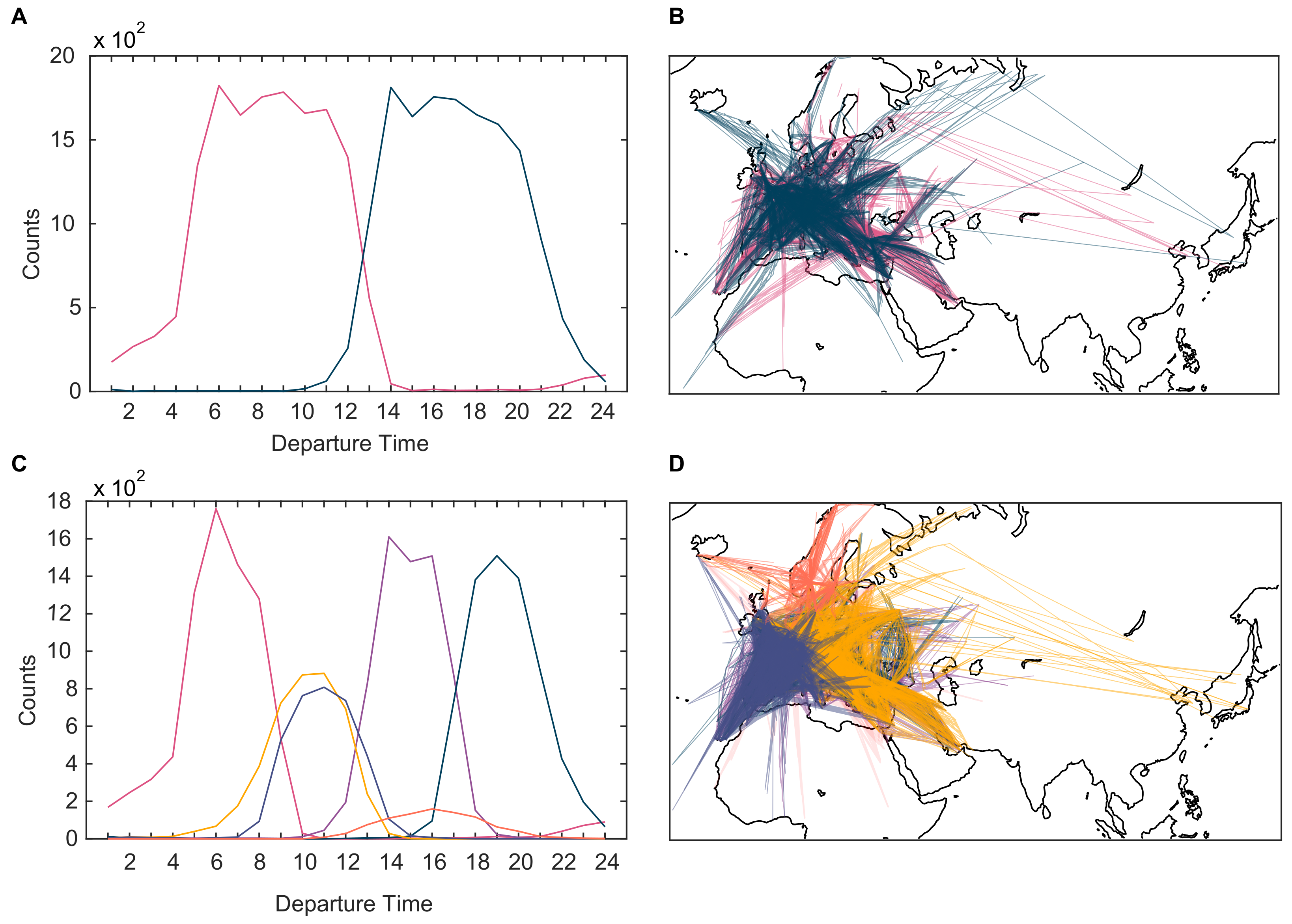
3.2. Temporal and Spatial Analysis of Clusters

To characterise the results of the partitioning algorithm, we looked at the temporal and spatial properties of the obtained clusters. Specifically, we looked at the distribution of departure times and at the spatial arrangement of the routes of flights contained in each cluster. We found that the clusters have a clear temporal or spatial characterisation. For example, in Figure 4A, we observe that the Infomap algorithm on network 1 finds two clusters with well-separated departure times. The two clusters are spatially overlapping (panel B). The Louvain algorithm on network 3, instead, finds clusters that have some temporal overlap (panel C). However, clusters that overlap temporally are spatially distinct. In fact, in panel D we see that the two clusters that both contain flights departing around 10 a.m. (yellow and dark violet) have different geographical positions. Similarly, the cluster that is temporally distributed along the entire afternoon and overlaps with two other clusters, is very specific geographically, being localised in the Scandinavian area. Results for other algorithms are in Supplementary Figures S2 and S3.

Therefore, we conclude that both community detection algorithms succeed in finding clusters of flights that have in common the time of the day, the geographical position, or both. The fineness of this separation depends on the algorithms and on the network. For example, the temporal division performed by the Infomap algorithm on network 1 (panel A) is rougher than the one performed by the Louvain algorithm on network 3 (panel C). The latter isolates four different time periods: early morning, late morning, early afternoon, and late afternoon.

3.3. A Trade-Off between the Number of Capacity Violations and the Resolution Time

We apply the SAIPE optimisation to each partitioned network obtained with the different scenarios. The optimisation is run in parallel on the clusters. For each run, we obtain an optimised strategic plan for each cluster, and by aggregating over clusters we obtain the global strategic plan for all flights.

The advantage that we expected in optimising independently the clusters was to have a reduced resolution time. Indeed, we find that the resolution time of the SAIPE decreases with the number of clusters (Figure 5A). This is expected because solving in parallel more, but smaller, clusters is faster than solving a smaller number of larger clusters. For any number of clusters, the resolution time is shorter than the time needed to find the global exact solution on the unpartitioned network, which is roughly 260s.

The advantage of a reduced resolution time must be evaluated in parallel to the disadvantage of obtaining an approximate global solution. To quantify the quality of this global solution, we measure the number and size of the violations of capacity constraints. Given a global solution, i.e., a strategic flight plan, we compare the sectors-hour occupation with the nominal capacities, to assess constraint violations. We call the violations computed according to the strategic flight plan strategic violations.

First, we look at the number of capacity violations, i.e., the number of sectors where the nominal capacity is exceeded. The number of violations tends to increase with the numbers of clusters (Figure 5B). This pattern means that when the network is partitioned in more clusters, it happens more often that two interacting flights are in two distinct clusters, and are therefore optimised independently.

There is therefore a trade-off between the number of violations, lower when there are few clusters, and the resolution time, lower when there are many clusters. Figure 5C shows that in the present case, a good trade-off is represented by Infomap on network 1. This scenario in fact reduces the resolution time by roughly one-third with respect to time needed to run the SAIPE on the entire network (baseline), at the cost of a small number of violations. Further reducing the resolution time comes at a higher relative cost in terms of violations.

The particular community detection method yielding the best solution might be specific to the problem. However, we can draw the general conclusion that partitioning flights in small number of clusters (3–5) represents a good compromise between reducing the resolution time and keeping the number of violations low.

We also compute the size of the violations, i.e., the number of flights exceeding the capacity, in absolute and in percentage. The mean and variance of the violation size do not show a dependence on the number of clusters and are similar for all scenarios (see Figure 6, blue bars). Infomap on network 2 shows the lowest mean violation size, both absolute and percentage.

3.4. Comparison with Actual Capacity Violations

To understand if the violations found in the approximate solutions produced by our approach are acceptable, we compare them with the violations that actually occurred on 1 September 2017. We find that the strategic violations are in all cases smaller in number and size with respect to the capacity violations that actually occurred on 1 September 2017 (represented as dotted lines in Figure 6). As explained in the Methods section (Section 2.6), a fairer comparison is that with the tactical violations that we estimate would arise from each strategic plan due to ATFM delays. These estimated tactical violations are more, in number, with respect to the strategic ones, but smaller on average (both in absolute value and in percentage) (see Figure 6, red bars). Importantly, they remain in all cases smaller in number and size with respect to the occurred violations. We can therefore conclude that, for all tested scenarios, the capacity violations produced by our approach are not a cause for concern.

4. Conclusions

The need for an air traffic system that is sustainable both from an environmental and an economic point of view requires the availability of mathematical and/or simulation models that allow to solve traffic management problems in a reasonable amount of time.

A classic approach to solving problems associated with complex systems consists of finding decompositions of the system in smaller subsystems that interact weakly with each other. In this work, we apply this approach to the set of flights, aiming to identify subsets of flights that interact as little as possible with other subgroups, where interactions are defined within the context of the specific problem at hand. Such decomposition allows to solve the problem independently on each of the subsystems. The resolution can thus be parallelised, with obvious computational advantages.

We partition the set of flights by applying community detection algorithms. To this end, the system must be appropriately formalised as a network, whose links represent the interactions that should be minimised between subsystems. We propose a method to build this network, with four possible variations, specifically for the problem of mitigating imbalances between capacity and demand. The methods use information available at the time of strategic flight planning on flights routes and departure times to identify which pairs of flights might interact during the resolution of the problem. The exact result of this partitioning depends on the method chosen to build the network and the clustering algorithm. However, analysing the clusters of flights that we obtained applying community detection algorithms to each of the networks, we found out that these clusters are temporally and/or spatially differentiated. This indicates that the minimisation of between-clusters interaction sought by the algorithms is consistently realised by gathering flights by temporal or spatial position.

We test four alternative methods to build the network and two clustering algorithms, which produce different results in terms of quality of the solution and computational time. We can use these differences to identify the most suited methodological choices. In the context of the present application, Infomap on network 1 offers the best combination of characteristics: low run time to perform the clustering and good trade-off between resolution time of the strategic flight planning model and number of capacity violations, their size also being significantly smaller than the realised ones. While this specific conclusion might not directly generalise to all datasets and problems, we can draw some general indications. First, in terms of capacity violations, all solutions for the problem of strategic flight planning obtained with any method and clustering algorithm are acceptable. In fact, all choices yield violations that are, in number and size, considerably smaller than the actual ones. Therefore, the quality of the solution should not be a strong concern in the choice of the method. Second, the shorter run time of the Infomap algorithm to perform the clustering make it preferable with respect to the Louvain algorithm. Third, if a good guess of the most likely trajectory is available (e.g., from historical data), it seems preferable to use methods 1 or 2 to build the network. In fact, these two methods require a shorter run time for the clustering (due to the smaller number of links) and yield either a better (in the case of Infomap) or comparable (in the case of Louvain) trade-off between violations and resolution time.

The results of this work also offer significant developments that might go beyond the simple reduction of computational resolution times. In fact, the possibility of identifying groups of flights that only weakly interact with each other allows, for example, to isolate the downstream effects that can be caused by a flight’s delay (reactionary delay) and also the consequences that it can have on passenger connectivity (missed connections). To perform this type of analysis, however, the definition of interaction between flights (used to establish links in the network) should be expanded. It should include not only interactions in the airspace, but also at airports, a study which is currently under development.

With the inclusion of interactions at airports, our approach could also lead to significant enhancements of models that optimise the allocation of airport slots. Currently, these slots are allocated according to the IATA World Schedule Guidelines (WSG) on an airport-by-airport basis. The allocation does not take place for a single day, but for a series of slots. A series is composed of at least five slots allocated for the same or approximately same time on the same day-of-the-week, distributed regularly in the season [32]. Since airports are clearly interconnected, the current single airport allocation is likely to produce allocations at two different airports that may not be compatible with the flight time between them. For this reason, twice a year, a Slot Coordination conference takes place principally to resolve conflicts stemming from the timing of slots allocated across multiple airports [33]. The current contributions that address the allocation of airport slots at the network level are based on very strong simplifications that severely limit their applicability—only for single days and not in series [34], with computer-generated instances under a number of severely simplifying assumptions [35], or considering a network composed of only 3 airports in southern China [36]. An appropriate decomposition of the network, as proposed in this work, could foster the development of optimisation models that limit the use of face-to-face and manually conducted negotiations, as is the case today in the Slot Coordination conference.

References

1. EUROCONTROL. Five-Year Forecast 2020–2024. European Flight Movements and Service Units. Three Scenarios for Recovery from COVID-19. 2020. Available online: https://www.eurocontrol.int/sites/default/files/2020-11/eurocontrol-five-year-forecast-europe-2020-2024.pdf (accessed on 6 August 2021).
2. EUROCONTROL. Performance Review Report. An Assessment of Air Traffic Management in Europe during the Calendar Year 2019. 2020. Available online: https://www.eurocontrol.int/publication/performance-review-report-prr-2019 (accessed on 6 August 2021).
3. EUROCONTROL. ATM Cost-Effectiveness (ACE) 2019 Benchmarking Report with Special Focus on COVID-19 Impacts in 2020. 2021. Available online: https://www.eurocontrol.int/sites/default/files/2021-05/eurocontrol-ace-2019-benchmarking-report-special-focus-covid-19-impact-2020.pdf (accessed on 6 August 2021).
4. European Aviation Environmental Report. 2019. Available online: https://ec.europa.eu/transport/sites/default/files/2019-aviation-environmental-report.pdf (accessed on 6 August 2021).
5. Delgado, L. European route choice determinants. In Proceedings of the 11th USA/Europe Air Traffic Management Research and Development Seminar, Lisbon, Portugal, 23–26 June 2015. [Google Scholar]
6. Ngo, D.; Shamoun, F. Environmental Cost of Different Unit Rates. Master’s Thesis, Linköping University, Linköping, Sweden, 2016. [Google Scholar]
7. Bolić, T.; Castelli, L.; Rigonat, D. Peak-load pricing for the European Air Traffic Management system using modulation of en-route charges. EJTIR 2017, 1, 136–152. [Google Scholar]
8. Verbeek, R.J.; Visser, H.G. Why aircraft will fly more fuel-efficiently on FRIDAY: The FRIDAY route charges method. In Proceedings of the 7th International Conference on Research in Air Transportation, Philadelphia, PA, USA, 20–24 June 2016. [Google Scholar]
9. Bertsimas, D.; Lulli, G.; Odoni, A. An integer optimization approach to large-scale air traffic flow management. Oper. Res. 2011, 59, 211–227. [Google Scholar] [CrossRef]
10. Sherali, H.D.; Hill, J.M.; McCrea, M.V.; Trani, A.A. Integrating Slot Exchange, Safety, Capacity, and Equity Mechanisms Within an Airspace Flow Program. Transp. Sci. 2011, 45, 271–284. [Google Scholar] [CrossRef]
11. Castelli, L.; Corolli, L.; Lulli, G. Critical Flights Detected with Time Windows. Transp. Res. Rec. 2011, 2214, 103–110. [Google Scholar] [CrossRef]
12. Agustín, A.; Alonso-Ayuso, A.; Escudero, L.; Pizzaro, C. On air traffic flow management with rerouting. Part I: Deterministic case. Eur. J. Oper. Res. 2012, 219, 156–166. [Google Scholar] [CrossRef]
13. Barnhart, C.; Bertsimas, D.; Caramanis, C.; Fearing, D. Equitable and Efficient Coordination in Traffic Flow Management. Transp. Sci. 2012, 46, 262–280. [Google Scholar] [CrossRef] [Green Version]
14. Bertsimas, D.; Gupta, S. Fairness and Collaboration in Network Air Traffic Flow Management: An Optimization Approach. Transp. Sci. 2015, 50, 56–76. [Google Scholar] [CrossRef]
15. Xu, Y.; Dalmau, R.; Melgosa, M.; Montlaur, A.; Prats, X. A framework for collaborative air traffic flow management minimizing costs for airspace users: Enabling trajectory options and flexible pre-tactical delay management. Transp. Res. Part B Methodol. 2020, 134, 229–255. [Google Scholar] [CrossRef]
16. Xu, Y.; Prats, X.; Delahaye, D. Synchronised demand-capacity balancing in collaborative air traffic flow management. Transp. Res. Part C Emerg. Technol. 2020, 114, 359–376. [Google Scholar] [CrossRef] [Green Version]
17. Ivanov, N.; Jovanović, R.; Fichert, F.; Strauss, A.; Starita, S.; Babić, O.; Pavlović, G. Coordinated capacity and demand management in a redesigned Air Traffic Management value-chain. J. Air Transp. Manag. 2019, 75, 139–152. [Google Scholar] [CrossRef]
18. Starita, S.; Strauss, A.K.; Fei, X.; Jovanović, R.; Ivanov, N.; Pavlović, G.; Fichert, F. Air Traffic Control Capacity Planning under Demand and Capacity Provision Uncertainty. Transp. Sci. 2020, 54, 882–896. [Google Scholar] [CrossRef]
19. Cook, A.; Blom, H.A.; Lillo, F.; Mantegna, R.N.; Miccichè, S.; Rivas, D.; Vázquez, R.; Zanin, M. Applying complexity science to air traffic management. J. Air Transp. Manag. 2015, 42, 149–158. [Google Scholar] [CrossRef] [Green Version]
20. Rocha, L.E. Dynamics of air transport networks: A review from a complex systems perspective. Chin. J. Aeronaut. 2017, 30, 469–478. [Google Scholar] [CrossRef]
21. Fleurquin, P.; Ramasco, J.J.; Eguiluz, V.M. Systemic delay propagation in the US airport network. Sci. Rep. 2013, 3, 1159. [Google Scholar] [CrossRef] [PubMed] [Green Version]
22. Gegov, E.; Postorino, M.N.; Atherton, M.; Gobet, F. Community structure detection in the evolution of the United States airport network. Adv. Complex Syst. 2013, 16, 1350003. [Google Scholar] [CrossRef]
23. Gurtner, G.; Vitali, S.; Cipolla, M.; Lillo, F.; Mantegna, R.N.; Miccichè, S.; Pozzi, S. Multi-Scale Analysis of the European Airspace Using Network Community Detection. PLoS ONE 2014, 9, e94414. [Google Scholar] [CrossRef] [Green Version]
24. Zaoli, S.; Mazzarisi, P.; Lillo, F. Trip Centrality: Walking on a temporal multiplex with non-instantaneous link travel time. Sci. Rep. 2019, 9, 10570. [Google Scholar] [CrossRef]
25. Bolić, T.; Castelli, L.; Corolli, L.; Rigonat, D. Reducing ATFM delays through Strategic Flight Planning. Transp. Res. Part E 2017, 98, 42–59. [Google Scholar] [CrossRef] [Green Version]
26. Blondel, V.D.; Guillaume, J.L.; Lambiotte, R.; Lefebvre, E. Fast unfolding of communities in large networks. J. Stat. Mech. Theory Exp. 2008, 2008, P10008. [Google Scholar] [CrossRef] [Green Version]
27. Rosvall, M.; Bergstrom, C.T. Maps of random walks on complex networks reveal community structure. Proc. Natl. Acad. Sci. USA 2008, 105, 1118–1123. [Google Scholar] [CrossRef] [Green Version]
28. Rand, W.M. Objective Criteria for the Evaluation of Clustering Methods. J. Am. Stat. Assoc. 1971, 66, 846–850. [Google Scholar] [CrossRef]
29. Cover, T.M.; Thomas, J.A. Entropy, Relative Entropy, and Mutual Information. In Elements of Information Theory; John Wiley & Sons, Ltd.: Hoboken, NJ, USA, 2005; Chapter 2; pp. 13–55. [Google Scholar]
30. Hubert, L.; Arabie, P. Comparing partitions. J. Classif. 1985, 2, 193–218. [Google Scholar] [CrossRef]
31. Vinh, N.X.; Epps, J.; Bailey, J. Information Theoretic Measures for Clusterings Comparison: Variants, Properties, Normalization and Correction for Chance. J. Mach. Learn. Res. 2010, 11, 2837–2854. [Google Scholar]
32. IATA. Worldwide Slot Guidelines, 10th ed.; IATA: Montreal, QC, Canada, 2019; Available online: https://www.iata.org/contentassets/4ede2aabfcc14a55919e468054d714fe/wsg-edition-10-english-version.pdf (accessed on 6 August 2021).
33. Ribeiro, N.A.; Jacquillat, A.; Antunes, A.P.; Odoni, A.R.; Pita, J.P. An optimization approach for airport slot allocation under IATA guidelines. Transp. Res. Part B Methodol. 2018, 112, 132–156. [Google Scholar] [CrossRef]
34. Pellegrini, P.; Bolić, T.; Castelli, L.; Pesenti, R. SOSTA: An effective model for the Simultaneous Optimisation of airport SloT Allocation. Transp. Res. Part E Logist. Transp. Rev. 2017, 99, 34–53. [Google Scholar] [CrossRef] [Green Version]
35. Benlic, U. Heuristic search for allocation of slots at network level. Transp. Res. Part C Emerg. Technol. 2018, 86, 488–509. [Google Scholar] [CrossRef]
36. Wang, D.; Zhao, Q. A simultaneous optimization model for airport network slot allocation under uncertain capacity. Sustainability 2020, 12, 5512. [Google Scholar] [CrossRef]
Figure 1. Outline of the proposed approach. (A) We consider the flights of a whole day in the European airspace. The trajectory of a flight is given by the list of sectors-hour it crosses. A sector-hour is a sector of the airspace associated to a time window of 1 h; (B) The trajectories of two flight overlap if they have sectors-hour in common; (C) A network of flights can be built, where two flights are linked if they are likely to influence each other in an optimisation process. A link is established using a criterion based on the overlapping of their trajectories. The network is then partitioned in weakly interacting clusters relying on popular community detection algorithms; (D) Optimising the whole network provides an exact solution, while satisfying all constraints on sector capacities, but it is computationally demanding. In the partitioned network, clusters can be optimised in parallel, saving computational time. A global solution is obtained by aggregating the solution of each cluster. The global solution can violate some constraints, however, if the clusters are weakly interacting the violations are expected to be small.
Sustainability 13 08924 g001
Figure 2. Results of the two community detection algorithms on the four considered networks. (A) Run time; (B) Number of clusters identified. Circles are outliers, crosses represent the data used to make the boxes.
Sustainability 13 08924 g002
Figure 3. Similarity of partitions, measured by Rand Index (red) and Mutual Information (blue). (A) Similarity of partitions across different runs of the same scenario. (B) Comparison of the similarity of partitions obtained with different runs of the same scenario and with different scenarios. Crosses represent the data used to make the boxes, circles are outliers. (C) Similarity of partitions obtained with different clustering methods on the same network. (D) Similarity of partitions obtained on two different networks with the same clustering method (above Infomap, below Louvain). For example, 1-2 refers to the comparison between results obtained on networks 1 and 2.
Sustainability 13 08924 g003
Figure 4. Temporal and spatial characterisation of clusters. (A) Histograms of departure times for clusters found by the Infomap algorithm on network 1. (B) Spatial distribution of clusters found by the Infomap algorithm on network 1. (C) Histograms of departure times for clusters found by the Louvain algorithm on network 3. (D) Spatial distribution of clusters found by the Louvain algorithm on network 3. In panels B and D, each segment represents a flight, and for each cluster, only 300 flights picked at random are represented, for clarity.
Sustainability 13 08924 g004
Figure 5. Results of application of SAIPE to outputs of community detection, for each of the 8 scenarios (30 runs of the community detection algorithm for each scenario). (A) Box plot of resolution time of SAIPE for each scenario, plotted against the average number of cluster obtained with that scenario. (B) Box plot of number of violations produced by SAIPE for each scenario, plotted against the average number of cluster obtained with that scenario. Circles are outliers, crosses represent the data used to make the boxes. (C) Average number of violations against average resolution time for each scenario and for the non-partitioned case (baseline). Error bars are standard deviations.
Sustainability 13 08924 g005
Figure 6. Number of violations, mean and variance of absolute and percentage size of violations for each scenario and from the empirical data. Blue bars represent strategic violations, values are averaged over 30 repetitions of the community detection algorithm (on whose results the SAIPE is applied). Red bars represent tactical violations, averaged over 30 repetitions of the community detection algorithms and over 3000 random delay assignments for each repetition. The dotted lines represent the number and size of violations occurred on 1 September 2017, respectively.
Sustainability 13 08924 g006
Publisher’s Note: MDPI stays neutral with regard to jurisdictional claims in published maps and institutional affiliations.