Climate Change Impact on the Hydrologic Regimes and Sediment Yield of Pulangi River Basin (PRB) for Watershed Sustainability

Abstract

The impacts of climate change are increasingly threatening the sustainability of ecosystems around the world. The Pulangi River Basin (PRB) in the Philippines is experiencing sedimentation beyond the tolerable amount (11.2 tons/ha/yr) due to land conversion and the effects of climate change. Changes in precipitation and temperature due to climate change are likely to further affect the annual runoff and sediment yield of PRB. In this study, the Soil and Water Assessment Tool (SWAT) was employed to simulate various scenarios of twelve downscaled climate projections from three Global Circulation Models (GCM) of CMIP5 under two Representative Concentration Pathways (RCP 4.5 and 6.0) for 2040–2069 and 2070–2099 timeframes, and the results were compared to a baseline period (1975–2005). This study revealed that the maximum mean annual precipitation is expected to increase by 39.10%, and the minimum and maximum temperatures are expected to increase by 3.04 °C and 3.83 °C, respectively. These observed changes correspond to an increase in runoff (44.58–76.80%) and sediment yield (1.33–26.28%) within the sub-basins. These findings suggest a general increase in the threat of severe flooding and excessive soil loss, leading to severe erosion and reservoir sedimentation throughout the PRB.

1. Introduction

The impacts of climate change on the environment and many societies around the world are considerable. Climate change is widely considered the most severe environmental issue we face. The United Nations established the Intergovernmental Panel for Climate Change (IPCC) in 1988 to assess the risks of climate change and deliver scientific information to governments and the different sectors in which policymakers are responsible for adapting and mitigating climate change. The IPCC has reported with medium confidence that the average of combined land and ocean surface temperature in a global scale is increasing in a linear trend, warming 0.85 °C from 1880 to 2012 [1]. The increase in precipitation after 1951 over the mid-latitude areas of the Northern Hemisphere has resulted from changes in many extreme weather and climate events. This observed global warming since the 1950s is due to the increased concentration of carbon dioxide and other gases in the atmosphere. Over the long term (2080–2100 at a global mean temperature increase of 2 °C and 4 °C) in Asia, the IPCC predicts the region, especially the Philippines, has a medium to very high risk of severe flooding [1].

Various researchers have studied the potential impact of climate change on water quality and quantity in river basins. Nguyen et al. (2020) investigated the impact of climate change on extreme rainfall and river flooding in the Ishikari River basin of Japan during the summer monsoon. The results showed that an extreme rainfall and severe river flooding events are expected to increase significantly in the future, with a 29–35% increase in rainfall and 37–56% increase in streamflow [2]. The climate change impact on stream discharge and sediment yield was evaluated by Azari et. al. (2016) in the Gorganroud River basin of Iran incorporating three GCMs with three Special Reports on Emission Scenarios (SRES AIF1, B1, and A2) [3]. The results of this study revealed a general increase in annual streamflow of 9.5% and that the sediment yield may increase by as much as 83.9% [3]. Mehan et al. (2016) demonstrated the risks of the dry condition in the Skunk Creek basin of South Dakota, USA in the mid-21st century due to temperature increase (2.2–3.3 °C), precipitation reduction (1.8–4.5%), and intense evaporation losses [4].

The climate change impact in several watersheds in Southeast Asia have been investigated using the SWAT Model. For instance, a simulation was performed for the climate change impact on the river discharge and suspended sediment load of Bangpakong River in Thailand employing six GCMs under the SRES-AIB emission scenario [5]. The results of this study showed a 1% increase in the period of 2040–2069 for both streamflow and sediment loads during the rainy season, and a decrease of about 3% for river discharge and 23% for sediment load during the dry season [5]. In a similar study on the influence of climate change on the hydrologic response of the Be River basin of Vietnam employing two SRES emission scenarios (A1B and B1) from the four ensemble GCMs, it was found that the future changes in annual temperature and precipitation tend to result in a warmer climate under most scenarios, and that the 2020s and the 2050s will be drier but the 2080s will be wetter [6]. From this observation, the annual streamflow during the wet season is expected to increase in the future, while the streamflow in the dry season is expected to decrease dramatically: this raises concerns about the high possibility of water shortage during the dry season [6]. In the other study by Tan et.al, 2017, the potential impact of climate change on the Kelatan river basin of Malaysia was also explored using thirty-six downscaled climate projections from five GCMs of Coupled Model Intercomparison Project Phase 5 (CMIP5) under three emission scenarios (RCP 2.5, 4.5, and 8.5) for the timeframes 2015–2044 and 2045–2074 [7]. Their finding indicates an increase of annual precipitation of 1.2–8.7% and a temperature increase of 0.6–2.1 °C that further results in an increase in annual runoff (46.8–90.2%), annual streamflow (14.6–27.2%), water yield (14.2–26.5%) and evapotranspiration (0.3–2.7%) [7].

In the Philippines, several studies have been conducted to assess the impact of climate change. The focus of one of these studies was on the impact of climate change and land use/land cover on the soil loss of the Cagayan River Basin with exploration of land-cover-based mitigation measures incorporating SRES-A1B and land use/land cover storylines [8]. A 37% increase was found in the sediment yield for the period 2036–2065 compared to the base scenario (1971–2000). Meanwhile, simulations incorporating land-cover-based mitigation measures through riparian reforestation and mountainous afforestation areas have shown that the intensity of soil loss can be reduced by a further 33% [8]. A SWAT model was also used to study the climate change impact on dependable flow and the potential irrigable area of the Maasin River watershed in Laguna [9]. The study revealed that the potential irrigable area is expected to decrease between 2006 and 2035 and between 2036 and 2065 because the reduction in dependable flow and increased irrigation water demand will result in a substantial shrinking of 57% to 97% of irrigable areas in the irrigation system within the Maasin river watershed [9]. Similarly, the SWAT model was also employed in three watersheds in the Philippines (Saug Watershed in Davao del Norte, Quiaoit river watershed in Ilocos Norte, and Pagsanjan-Lumban watershed in Laguna) to assess the hydrologic response of climate and land-cover changes [10]. The conclusion of this study was that changes in climate and land cover will likely affect the hydrological balance of the watershed, and it also showed a significant increase in surface runoff that may cause severe erosion, reservoir sedimentation, soil nutrients depletion, and flooding in low-lying areas of watersheds [10]. In 2011, the Philippine Atmospheric, Geophysical, and Astronomical Services Administration (PAGASA) assessed the climate change impact in the Philippines. The PAGASA projected the annual mean and seasonal temperature changes, minimum and maximum temperature changes, seasonal rainfall changes, and frequency of extreme events for timeframes centered on the 2020s (2006–2035) and 2050s (2036–2065) using the PRECIS model software incorporating the SRES scenarios (A2 (high-range), A1B (mid-range), and B2 (low-range)) from ECHAM4 and HadCM3Q0 regional climate models [11]. The assessment revealed that the Philippines would become warmer, especially during the summer period (June, July, August). The mean temperature is expected to rise by 1.8 °C to 2.2 °C in the 2050s, and a reduction in rainfall will likely occur throughout the country. The same study showed that extreme temperature events (exceeding 35 °C) and heavy daily rainfall (exceeding 300 mm) will be more frequent in the future, and extreme rainfall events are projected to increase mainly in Luzon and Visayas. The projected changes in temperature and precipitation in the country are likely to result in water stress in terms of both quantity and quality, and cascade into more adverse impacts. Despite this effort, climate change assessment in the Philippines is still limited. Further studies are required to develop a better understanding of the potential impacts of climate change on the hydrological systems and diverse ecosystems in the Philippines. One of the methods to gather this kind of information is to apply RCP emission scenarios to analyze the impacts of changing climate.

Besides the expected adverse effects on the hydrological systems, climate change is also expected to influence the soil characteristics. Rainfall–runoff interactions are the essential factor for soil erosion and sediment yield [3]. Surface runoff carries sediments that are natural products of erosion. Because the sediment yield in a basin varies from time to time and from point to point, the stream is a natural transporter of both water and sediment [12]. It has been reported that the rate of soil loss in the Pulangi River Basin (PRB) in Mindanao, Philippines is beyond the tolerable amount of 11.2 tons/ha/yr in all of its sub-basins because of land conversion and plantation [13,14]. It is highly likely that climate change has also exacerbated the rate of soil loss in PRB. This soil loss has also affected the Pulangi reservoir, with the increase in sedimentation in effect limiting its storage volume to only 33% of its original storage capacity [15]. Excessive soil loss threatens the sustainability of watersheds, including reservoir operation, land, and water resources. Understanding the potential changes in runoff and sediment yield in a particular watershed is essential to develop effective mitigation and adaptation plans for watershed management development. Therefore, in this study, the impact of climate change on the annual runoff and sediment yield in the PRB was investigated using the Soil and Water Assessment Tool (SWAT). Because climate scenarios are highly relevant in the IPCC adaptation approach [16,17], twelve climate change projections were downscaled from three GCMs (GFDL-ESM2M, HadGEM2-ES, and MIROC) of CMIP5 for the timeframes 2040–2069 and 2070–2099 under the Representative Concentration Pathway (RCP 4.5 and 6.0) for use in the SWAT model. The results of the study are expected to provide a helpful scientific reference for policymakers in implementing measures to adapt to climate change and adopt mitigation measures in the PRB.

2. Materials and Methods

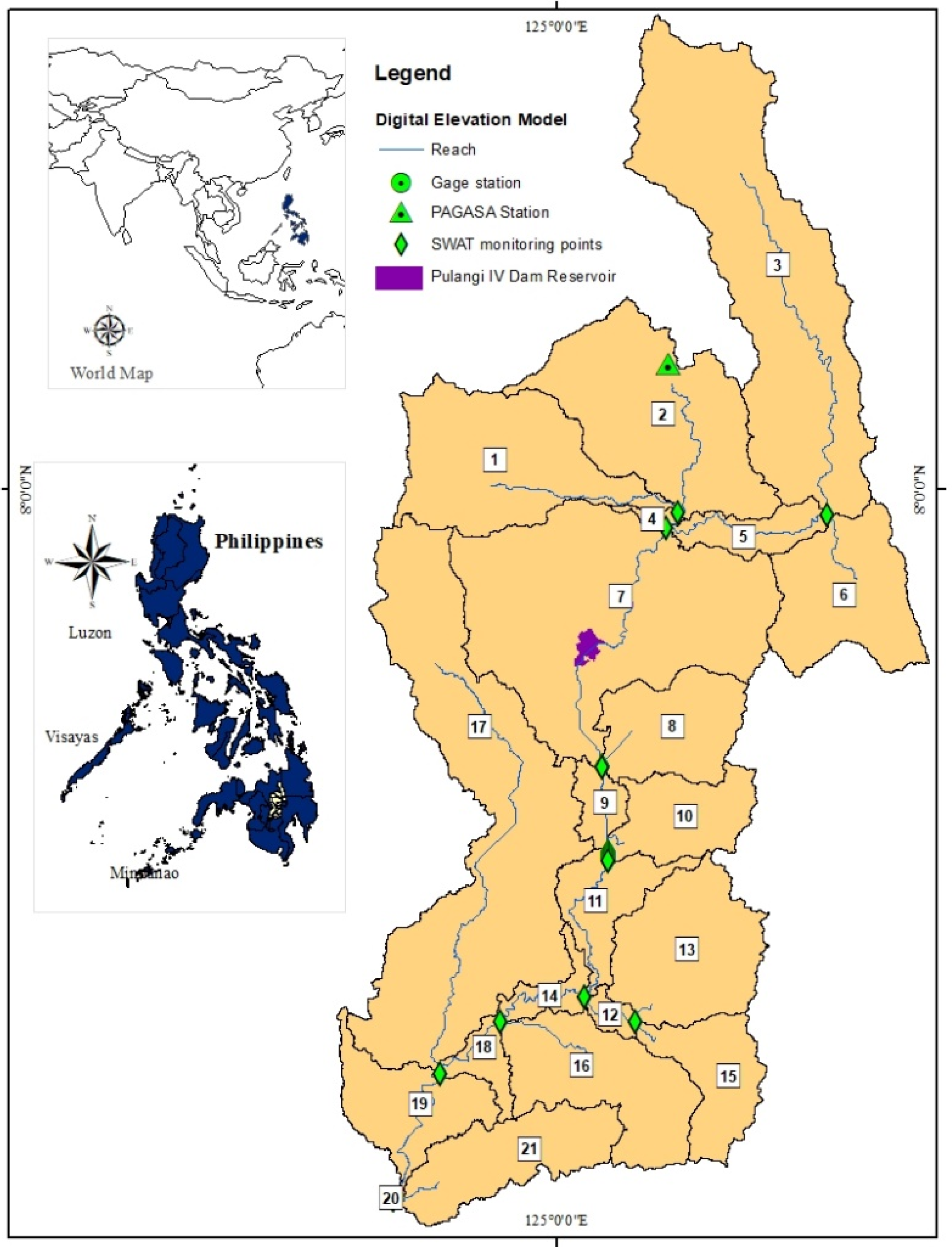
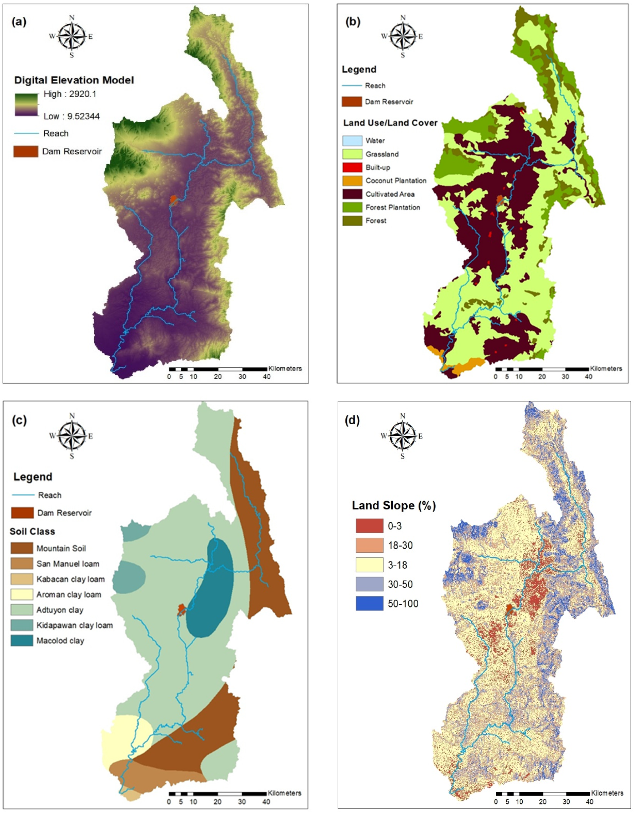
The methodology developed by the authors in this study is shown in Figure 1. In this figure, the processes, datasets, and tools used in the model are presented. The SWAT model requires several inputs to generate the base and climate change scenario for the climate change analysis. Information about the meteorological data and spatial data, including vegetation, topography, soil properties, land management practices, and relevant to the watershed is the primary input to the SWAT model, and is necessary to analyze the physical processes of water and sediment movement [18]. A sensitivity analysis, model calibration and validation were done using Calibration Uncertainty Program for SWAT (SWAT-CUP) by employing processed data and observed data (streamflow and soil erosion rate) as an input to produce the calibrated model. For climate change data preparation, three GCMs were extracted from CMIP5 to build different climate change scenarios. In this study, bias correction and statistical downscaling were carried out to ensure the quality of the model output, followed by interpolation using the Inverse Distance Weighted (IDW) method to extract a finer resolution for a more appropriate regional climate assessment.

2.1. Study Area

The study area is the Pulangi River Basin (PRB), which is located in the Mindanao Island of the Philippines, shown in Figure 2. The river has a length of 320 km and a delineated watershed area of approximately 6500 km² that traverses most cities and municipalities in the Bukidnon Province in Region 10 and the Cotabato Province of Region 12. The PRB was subdivided into 21 sub-basins and 681 Hydrological Response Unit (HRUs). The Pulangi watershed has a Hydroelectric Power Plant (HEPP) located on the upper part of its watershed powered by a dam reservoir with 67 million cubic meters (mcm). The elevation of the PRB ranges from 9.52 to 2920 m above sea level (masl). The slope of nearly 90% of the catchment is greater than 18%. Because most upstream areas are located within the hillslope of Mount Kitanglad, the highest elevation is the Manupali subwatershed. The climate in this region is relatively cool and humid throughout the year, with an average rainfall of 2800 mm. Rainfall is heaviest from June to October, and February to April are the drier months. The recorded temperature ranges from 20 to 34 °C at elevations less than 500 masl and from 18 to 28 °C for elevations above 500 masl.

2.2. Input Data

Meteorological and Geographic Information System (GIS) datasets were obtained from various sources to calibrate and validate the hydrological model and simulate climate change scenarios. A synthetic aperture radar-digital elevation model (SAR-DEM) with 10 m spatial resolution was acquired from the LiDAR Portal (link: https://lipad.dream.upd.edu.ph/ (accessed on 8 May 2020)) of the University of the Philippines Training Center for Applied Geodesy and Photogrammetry (UP-TCAGP) with the Department of Science and Technology (DOST) [19]. In this study, DEM was projected with the Universal Transverse Mercator (UTM) Zone 51 projection and World Geodetic System (WGS) 1984 as the horizontal datum, as shown in Figure 3a. A 30 m spatial resolution land use/land cover of PRB was retrieved from the National Mapping and Resource Information Authority (NAMRIA) (link: http://www.namria.gov.ph/ (accessed on 19 June 2020)), as presented in Figure 3b. The HRU simulation showed a total watershed area of 645,560.75 ha comprising the grassland area (46.03%), cultivated area (33.49%), forest area (10.0%), forest plantation (8.90%), built-up (0.20%), water (0.09%) and coconut plantation (1.29%). The soil properties of the basin and slope derived from the DEM are essential inputs to the SWAT model and determine the flow of water within the HRUs. The required soil parameters were derived from the digital soil world data of Food and Agricultural Organization (FAO) (link: http://www.fao.org/home/en/ (accessed on 20 July 2020)) and incorporated in the Philippine Soil Map acquired from the Bureau of Soil and Water Management (BMWS) of the Department of Agriculture (link: http://bswm.da.gov.ph/ (accessed on 21 July 2020)). The data was slightly modified so that it would be consistent with the SWAT database format. The soil reclassification in the SWAT analysis was classified as mountain soil (23.24%), Kidapawan clay loam (3.15%), Macolod clay (7.56%), Aroman clay loam (4.98%), San Manuel loam (4.37), Kabacan clay loam (0.53%), and predominated by Adtuyon clay (56.16%), as reflected in Figure 3c. The reclassified slopes were divided into six categories with their area percentage presented in the following figures: 0–3 as flat to nearly flat (9.37%), 3–18 as gently sloping to rolling (46.60%), 18–30 as rolling to hilly (20.69%), 30–50 as steep hills to mountainous (16.67%), and 50–9999 as very steep hills and mountains (6.68%), as presented in Figure 3d. The SWAT model requires data for precipitation, temperature, wind speed, relative humidity, and solar radiation [18]. Long-term observed datasets were acquired from PAGASA (link: http://bagong.pagasa.dost.gov.ph/climate/climate-data (accessed on 17 April 2020)) and were extracted from the Malaybay meteorological station with a geographical location of 8.151421 N 125.133852 E and elevation of 627 m, as seen in Figure 2 of PAGASA station, and represent 57 years of daily weather records from 1961 to 2018.

2.3. Climate Scenarios

Climate scenarios are considered vital in assessing not only impact of the changing climate but also vulnerability to climate change and adaptation to it. These scenarios provide an alternative projection of future conditions [11]. Thus, climate data at various temporal and spatial scales are essential for simulations. The climate projections were downscaled from the different General Circulation Model (GCM) obtained from CMIP5. The GCMs are numerical models illustrating the physical processes and characterics of the atmosphere, ocean, cryosphere, and land surface that are often employed to create future projections based on specific greenhouse gas (GHG) emission scenarios, and they are produced by Representative Concentration Pathways (RCPs) [17]. The GCMs was used in this research are GFDL-ESM2M, HadGEM2-ES, and MIROC, as shown in

Table 1. List of GCMs utilize in the study.

	Model	Institution	Country	Resolution
GCM1	GFDL-ESM2M	NOAA/Geophysical Fluid Dynamics Laboratory	United States	0.5° × 0.5°
GCM2	HadGEM2-ES	Met Office Hadley Center	United Kingdom	0.5° × 0.5°
GCM3	MIROC	AORI, NIES and JAMSTEC	Japan	0.5° × 0.5°

. The historical baseline period used to compare the downscaled climate data with observed data of precipitation and temperature is 1975–2005.

In 2014, the IPCC released its Fifth Assessment Report on climate change. They developed the Representative Concentration Pathways (RCP) representing the four different pathways of GHG emissions and atmospheric concentration, air pollution, and land use conditions in the 21st century for climate projections that support the adaptation and impacts assessment [1]. The four climate scenarios of RCPs represent the range of GHG emissions: RCP2.6 (the stringent mitigation scenario), RCP4.5 and RCP6.0 (two intermediate scenarios), and RCP8.5 (very high GHG emissions). The RCP 2.6 scenario is described as the peak radiative forcing ~3 W/m² (equivalent to ~490 ppm CO²) before 2100 and declining to 2.6 W/m² by 2100. The RCP 4.5 scenario is a stabilization without an overshoot pathway to 4.5 W/m² (or ~650 ppm CO² equivalent) at stabilization after 2100. The RCP 6.0 scenario is a stabilization without an overshoot pathway to 6 W/m² (or ~850 ppm CO² equivalent) at stabilization after 2100, and the RCP 8.5 scenario describes a rising forcing pathway leading to 8.5 W/m² (or ~1370 ppm CO² equivalent) by 2100 [20]. Thus, this study used RCP4.5 and RCP 6.0 for the simulation of climate change.

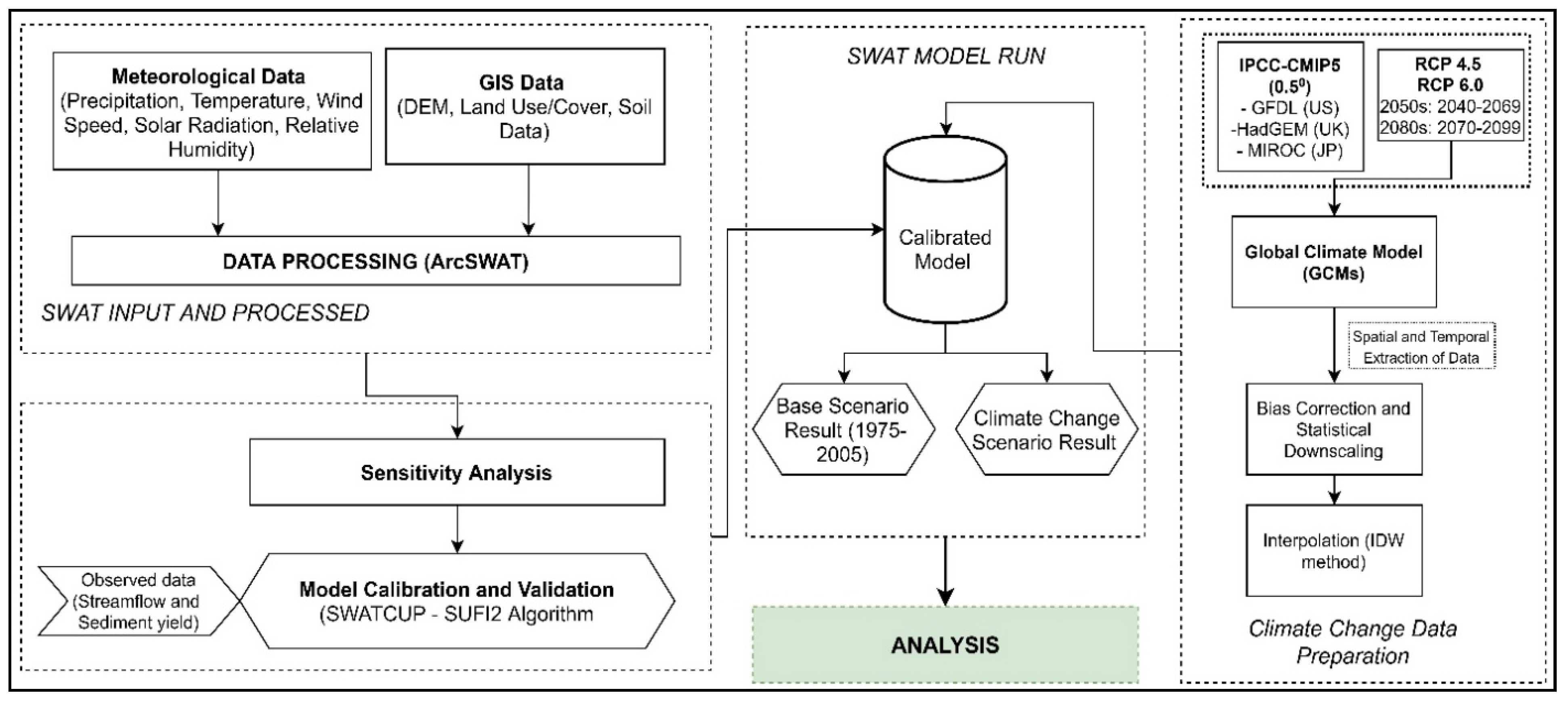
2.4. Model Set-Up for Calibration and Validation

The observed river discharges and sediment yield of the Pulangi river were used for the calibration and validation processes, as shown in Figure 2 (Gage station). The streamflow discharge datasets composed of 1983–2003 and 2009–2010 were acquired from the Department of Public Works and Highways (DPWH) [21]. The soil erosion rate of the Pulangi sub-basins for 2014–2015 was obtained from the National Power Corporation in the Philippines (https://www.napocor.gov.ph/ (accessed on 16 October 2020)) and supplemented by the experimental study of Marin and Jamis (2017) on the soil erosion observation of the three subwatersheds within the PRB [22].

The model performance was evaluated using the statistical indexes recommended by Moriasi et al., (2007) [23] using the Nash Sutcliffe efficiency (NSE), coefficient of determination (R2), Kling-Gupta efficiency (KGE), the ratio of the root mean square error (RMSE) to the standard deviation of observed data (RSR), and percent bias (PBIAS, as summarized in

Table 2. Summary of SWAT general performance ratings for recommended statistics for the monthly time step.

					PBIAS (%) (Moriasi et al., 2007)
Performance Rating	NSE (Moriasi et al., 2007)	R2 (Santhi et al., 2001)	KGE (Brighenti et al., 2019)	RSR (Moriasi et al., 2007)	Streamflow	Sediment
Very Good	0.75 < NSE ≤ 1.00	-	-	0.00 < RSR ≤ 0.50	PBIAS < ±10	PBIAS < ±15
Good	0.65 < NSE ≤ 0.75	-	KGE ≥ 0.7	0.50 < RSR ≤ 0.60	±10 ≤ PBIAS < ±15	±15 ≤ PBIAS < ±30
Satisfactory	0.50 ≤ NSE ≤ 0.65	R2 ≥ 0.5	0.5 ≤ KGE < 0.70	0.60 < RS ≤ 0.70	±15 ≤ PBIAS < ±25	±30 ≤ PBIAS < ±55
Unsatisfactory	NSE < 0.50	R2 < 0.50	KGE < 0.50	RSR > 0.70	PBIAS ≥ ±25	PBIAS ≥ ±55

). The NSE is a widely used objective function to test the application of hydrological model [22,23,24,25], and it was computed using Equation (1) [26]. The NSE is a normalized measure for ranges between −∞ to 1.0 (where 1.0 denotes ideal simulation, a zero represents average performance, and below zero represents unsatisfactory model) that compares the mean square error generated by a specific model simulation to the variance of the aim output sequence [27]. An NS value ≥ 0.5 was considered acceptable performance for streamflow and sediment yield, and ≤0.5 was considered unsatisfactory model performance [23]. The R² is a statistical measure on the robustness of the relationship between simulated and observed values represented in Equation (2). In general, values of R² ≥ 0.5 are satisfactory model performance while values ≤ 0.5 are unsatisfactory model simulation [28]. The KGE is the combination of the three components of NSE of the model errors $(r, \propto$, $\beta )$ represented in Equation (3), which is the conventional method for the calibration and evaluation of hydrological models [29]. The RSR is the standardized RMSE utilizing the standard deviation of the observations and combines both an error-index and the additional information suggested by Legates and McCabe (1999) [23,30], as expressed in Equation (4). The optimal value recommended for RSR is closer to zero, with values ≤ 0.70 considered acceptable performance while values ≥ 0.70 indicate unsatisfactory model simulations [23]. Moreover, the PBIAS measures the trend of the average of the simulated values and observed ones, given in Equation (5). The optimal value of PBIAS is zero; a value of ≤ ±15 for streamflow and ≤ ±30 for sediment is an indication of good model performance; and values ≥ ±25 for streamflow and ≥ ±55 for sediment indicate unsatisfactory model simulation [23]:

$$NSE=1-\left(\frac{{{\displaystyle \sum }}_{i=1}^n{\left(Q_i^{obs}-Q_i^{sim}\right)}^2}{{{\displaystyle \sum }}_{i=1}^n{\left(Q_i^{obs}-Q_i^{mean}\right)}^2}\right)$$

(1)

$$R^2=\frac{{\left({{\displaystyle \sum }}_{i=1}^n\left(Q_{sim}-Q_{m,sim}\right)\left(Q_{obs}-Q_{m,obs}\right)\right)}^2}{{{\displaystyle \sum }}_{i=1}^n{(Q_{sim}-Q_{m,sim})}^2 {{\displaystyle \sum }}_{i=1}^n{(Q_{obs}-Q_{m,obs})}^2}$$

(2)

$$KGE=1-\sqrt{{\left(r-1\right)}^2+{\left(\propto -1\right)}^2+{\left(\beta -1\right)}^2}$$

(3)

$$RSR=\frac{\sqrt{{{\displaystyle \sum }}_{i=1}^n{\left(Q_{obs,i}-Q_{sim,i}\right)}^2}}{\sqrt{{{\displaystyle \sum }}_{i=1}^n{\left(Q_{obs,i}-Q_{mean,}\right)}^2}}$$

(4)

$$PBIAS=\left(\frac{{{\displaystyle \sum }}_{i=1}^n{\left(Q_i^{obs}-Q_i^{sim}\right)}^2}{{{\displaystyle \sum }}_{i=1}^n{Q}_i^{obs}}\right)\times 100$$

(5)

where$Q_i^{obs} \& Q_{obs}$ are the observed values; $Q_i^{sim} \& Q_{sim}$ are simulated values; $Q_i^{mean} \& Q_{m,obs}$ are the mean of n observed values; $Q_{m,sim}$ is the mean of n simulated values; $r$ is the linear regression coefficient between observed and simulated values in which 1.0 is the ideal value; ∝ is the ratio of the standard deviation of simulated and observed values; and β is the ratio of the mean of the simulated and mean of the observed values.

2.5. Hydrological Modeling

SWAT is a physical-based continuous time model developed by the United States Department of Agriculture-Agricultural Research Service and Texas A&M University to assist water resource modelers to evaluate the impact of land management application on water supplies and nonpoint source pollution in watersheds and large river basins with diverse soils, and land use management over a long period [16,31]. SWAT with an Arc-GIS interface was utilized to model the PRB and simulate climate change. In SWAT, the watershed was segmented into several sub-basins and further discretized into a smaller unit within the sub-basin that contains a distinct combination of soil type, land slope, land use/cover properties, and is referred to as the Hydrological Response Unit (HRU). In this study, the PRB watershed was subdivided into 21 sub-basins and 684 HRUs.

The hydrological processes simulated in SWAT are based on the water balance equation expressed in Equation (6).

$$S{W}_t=S{W}_o+{{\displaystyle \sum }}_{i=1}^t\left(R_{day}-Q_{surf}-E_a-W_{seep}-Q_{qw}\right)$$

(6)

where $S{W}_t$ is the final soil water content (mm), $S{W}_o$ is the initial soil water content on day i (mm), t is the time in days, $R_{day}$ is the amount of precipitation on day i (mm), $Q_{surf}$ is the amount of surface runoff on day i, $E_a$ is the amount of evapotranspiration on day i (mm), $W_{seep}$ is the amount of water entering the vadose zone from the soil profile on day i (mm), and $Q_{qw}$ is the amount of return flow on day i (mm). SWAT simulates the surface runoff volumes and peak runoff rates for each HRU using the daily and subdaily rainfall amounts. The Soil Conservative Service (SCS) curve number method in Equation (7) was used in this study to estimate the amounts of runoff as a function of soil permeability, land use/cover, and soil water conditions:

$$Q_{surf}={\left(R_{day}-I_a\right)}^2/{\left(R_{day}-I_a+S\right)}^2$$

(7)

$$S=25.4\times \left(\frac{1000}{CN}-10\right)$$

(8)

where $Q_{surf}$ is the accumulated runoff or rainfall excess (mm), $R_{day}$ is the rainfall depth for the day (mm), $I_a$ is the initial abstractions which include surface storage, interception, and infiltration before the runoff (mm), and S is the retention parameter. The retention parameter (S) is expressed in Equation (8), and varies temporally and spatially due to the changes in soils, land use management, and slope due to the changes in soil water content, where CN is the curve number. The initial abstractions ($I_a$) in Equation (7) are approximated as 0.2 of the retention parameter (S). Moreover, sediment yield in SWAT is estimated for each HRU using the Modified Universal Soil Loss Equation (MUSLE) developed by Williams and Berndt, 1977 [32]. MUSLE uses runoff to simulate the erosion and sediment yield, as expressed in Equation (9).

$$Sed=11.8\times \left(Q_{surf}·q_{peak}·Are{a}_{hru}\right){ }^{0.56}· K_{USLE}·C_{USLE}·P_{USLE·}L{S}_{USLE}· CFRG$$

(9)

where $Sed$ is the sediment yield on a given day (metric tons), $Q_{surf}$ is the surface runoff volume (mm/ha), $q_{peak}$ is the peak runoff rate (m³/s), $Are{a}_{hru}$ is the area of the HRU (ha), $K_{USLE}$ is the USLE soil erodibility factor (0.013 metric tons m² hr/m³-metric ton cm), $C_{USLE}$ is the USLE cover and management factor, $P_{USLE.}$ is the USLE support practice factor, $L{S}_{USLE}$ is the USLE topographic factor, and $CFRG$ is the coarse fragment.

2.6. Bias Correction, Statistical Downscaling, and Interpolation

Spatial downscaling and the bias correction of GCM data are essential processes before conducting the regional climate change impact assessment. This study conducted bias correction due to the currently available GCM output, which consists of significant biases that can lead to substantial inaccuracy in regional impact evaluation if not corrected. The smaller the bias, the higher the model skill to simulate the observed climate accurately.

While GCMs are the main source of future climate data, their resolution is often too coarse for regional impact assessment [33]. Thus, downscaling is essential to extract finer spatial and temporal resolution from course resolution. There are two common methods for downscaling GCM data: statistical downscaling and dynamic downscaling (Regional Climate Model) [17]. The statistical downscaling approach adopted in this study used the widely used change factor method [23,24] due to its efficiency to downscale many GCM outputs to a finer spatial and temporal scale, and because it is computationally inexpensive and allows quick execution [34]. The change factor approach consists of adjusting the observed daily temperature ($T_{obs,d}$) by adding the difference of the monthly temperature of GCM between 2050s/2080s and the reference point $\left({\overline{T}}_{GCM,2050s\&2080s,m}-{\overline{T}}_{GCM,ref,m}\right)$ to generate the daily temperature for the 2050s/2080s horizon ($T_{corrected,fut,d}$) as expressed in Equation (10). The corrected daily precipitation for the 2050s/2080s horizon $\left(P_{corrected,fut,d}\right)$ is generated by multiplying the precipitation ratio $\left({\overline{P}}_{GCM,2050s\&2080s,m }/{\overline{P}}_{GCM,ref,m}\right)$ with the observed daily precipitation ($P_{obs,d}$), as shown in Equation (11).

$$T_{corrected,fut,d}=T_{obs,d}+\left({\overline{T}}_{GCM,2050s\&2080s,m}-{\overline{T}}_{GCM,ref,m}\right)$$

(10)

$$P_{corrected,fut,d}=P_{obs,d}\times \left({\overline{P}}_{GCM,2050s\&2080s,m}/{\overline{P}}_{GCM,ref,m}\right)$$

(11)

For interpolation, the Inverse Distance Weight (IDW) was utilized in this study to spatially interpolate the GCM grid points with the target station to acquire daily higher-resolution gridded datasets from 0.50 databases. Geoscientists and geographers widely use IDW due to its straightforward interpretation and easy computation method. IDW use a weighted combination of a set of available grids to determine new grid values [33]. It assumes that the unsampled point from an attribute value is the weighted mean of identified values contained by the grid cell, and the weights are inverse to the distances of the prediction point and sample point expressed in Equation (12) according to Lu and Wong (2008) [33,35], where $\widehat{y}\left(S_0\right)$ is the unknown value in the location $S_0$, given the observed y values at sampled locations $S_i$. This study interpolated daily temperature and rainfall data of the 0.5° grid using the IDW method to produce a 0.25° grid data set, equivalent to a 28 km resolution.

$$\widehat{y}\left(S_0\right)={{\displaystyle \sum }}_{i=1}^n\frac{1}{n}y \left(S_i\right)$$

(12)

3. Results and Discussion

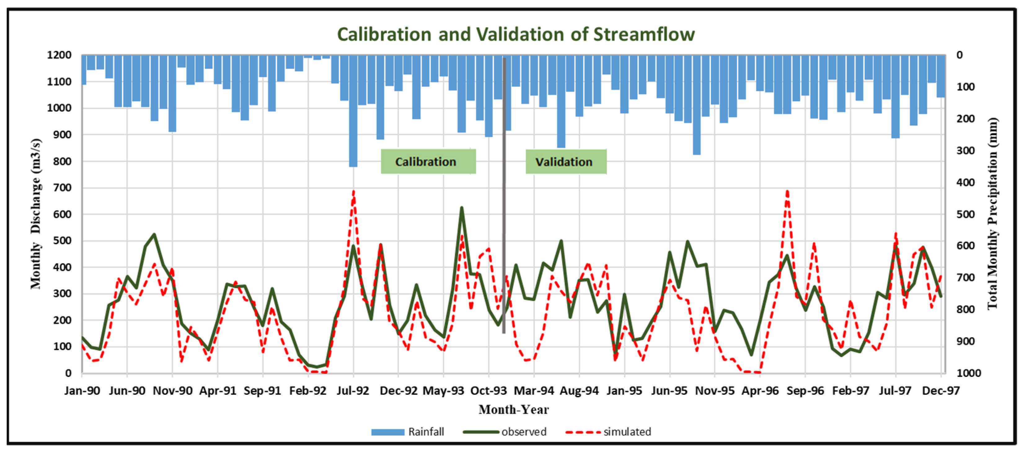
3.1. Sensitivity Analysis, Model Calibration, and Validation

The purpose of the sensitivity analysis is to determine the sensitive parameters involved in the process of the model. It is also a way to optimize the model results by adjusting the values of sensitive parameters based on the limit set by the SWAT. The calibration process is a statistical analysis of the set of parameters used in SWAT models to improve model results. The validation is a method of confirming the results of adjustment from the calibration process.

Model calibration in a watershed is quite challenging for modelers due to the uncertainties and process simplification [36]. These uncertainties are conceptual models from simplification and processes, input uncertainty on errors in input variables, and parameter uncertainty due to the inherent unexceptional inverse model parameters [37]. Moreover, the model development itself is a source of uncertainty, specifically with less familiarity in the landscape of the study area and insufficient understanding of various parameters and concepts used in SWAT. In this analysis, considerable effort was made to reduce these possible uncertainties by carefully considering the current dynamics of data accessibility. Unfortunately, no data specific to Pulangi Dam was incorporated in the PRB model simulation due to the lack of availability and the insufficient nature of the datasets available on dam operation.

Calibration and a sensitivity analysis were carried out by the initially considered 32 parameters using the Sequential Uncertainty Fitting (SUFI-2) algorithm of SWAT-CUP. For the fifth (last) iteration, only 12 parameters were found to be sensitive to streamflow and sediment yield, as shown in

Table 3. Calibrated value of SWAT parameters for streamflow and sediment yield.

Rank	Parameter	Description	Fitted Value	Min	Max	t-Stat	p-Value
1	R__CN2.mgt	Effective hydraulic conductivity in main channel alluvium	0.3854	0.2503	0.459	24.28	0
2	R__SOL_AWC(..).sol	Saturated hydraulic conductivity	1.1534	0.769	1.177	13.67	0
3	R__HRU_SLP.hru	Average slope length	0.6360	0.4950	0.660	4.02	0
4	V__GW_DELAY.gw	Groundwater delay (days)	374.5027	171.745	380.2	3.01	0
5	R__CNCOEF.bsn	Plant ET curve number coefficient	1.7640	0.8910	1.822	−1.97	0.05
6	R__USLE_P.mgt	USLE Equation support practice factor	1.0319	0.801	1.169	−1.55	0.12
7	R__CH_N2.rte	Manning’s “n” value for the main channel	0.2274	0.1300	0.238	1.54	0.13
8	R__OV_N.hru	Manning’s “n” value for overland flow	0.2643	0.2640	0.570	−1.34	0.18
9	R__SPCON.bsn	Linear parameter for calculating the maximum amount of sediment that can be re-entrained during channel sediment routing	0.0098	0.0070	0.01	−1.18	0.24
10	R__ESCO.hru	Soil evaporation compensation factor	0.6782	0.558	0.930	−1.09	0.28
11	V__GWQMN.gw	Threshold depth of water in the shallow aquifer required for return flow to occur (mm)	0.5582	−0.3320	0.628	−0.87	0.39
12	R__SURLAG.bsn	Surface runoff lag time	−7.9667	−14.5763	−2.720	−0.81	0.42

. Each iteration performed 300 model calls for a total of 1500 simulations. Table 3 also shows the list of sensitive parameters ranked according to their sensitivity levels with ranges of parameters based on t-stat and P-value. The relative significance of each model parameter is determined by the P-value and t-Stat of SUFI-2 algorithm [38]. The t-stat is the ratio of parameter coefficient to its standard error, and p-value, less than or equal to 0.05, is taken as a sensitive parameter. The CN2, SOL_AWC, HRU_SLP, GW_DELAY, and CNCOEFF are the most sensitive parameters in the simultaneous model simulation of streamflow and sediment yield.

Both the monthly observed and simulated streamflow of PRB for calibration and validation are shown in Figure 4 for comparison purposes. Monthly streamflow discharge and sediment yield as an objective function was used for model calibration and validation. The streamflow calibration resulted in a value of 0.72, 0.59, 0.77, 0.64, and 11.6 for the R², NSE, KGE, RSR, and PBIAS, respectively. This streamflow calibration outcome generally indicates a good performance for streamflow calibration based on SWAT general performance ratings, as displayed in Table 2. Meanwhile, the validation of streamflow has a value of 0.51, 0.42, 0.57, 1.15, and 19.4 for the R2, NSE, KGE, RSR, and PBIAS, respectively. While the NSE and RSR resulted in an unsatisfactory model, the performance of PBIAS, R2, and KGE was good to satisfactory. For the sediment yield calibration, the R², NSE, KGE, RSR, and PBIAS have a value of 0.42, 0.53, 0.48, 1.59, and 43.5, respectively. These showed that only the NSE index is satisfactory and that the other indicators are unsatisfactory. Meanwhile, in the sediment yield validation, the statistical indices R², NSE, KGE, RSR, and PBIAS have a value of 0.39, 0.44, 0.36, 1.72, and 47.4, respectively. The performance of R², NSE, KGE, and RSR was unsatisfactory while that of PBIAS was satisfactory. In general, model calibration and validation of sediment yield indicated unsatisfactory performance. This was attributed to to the limited availability of datasets.

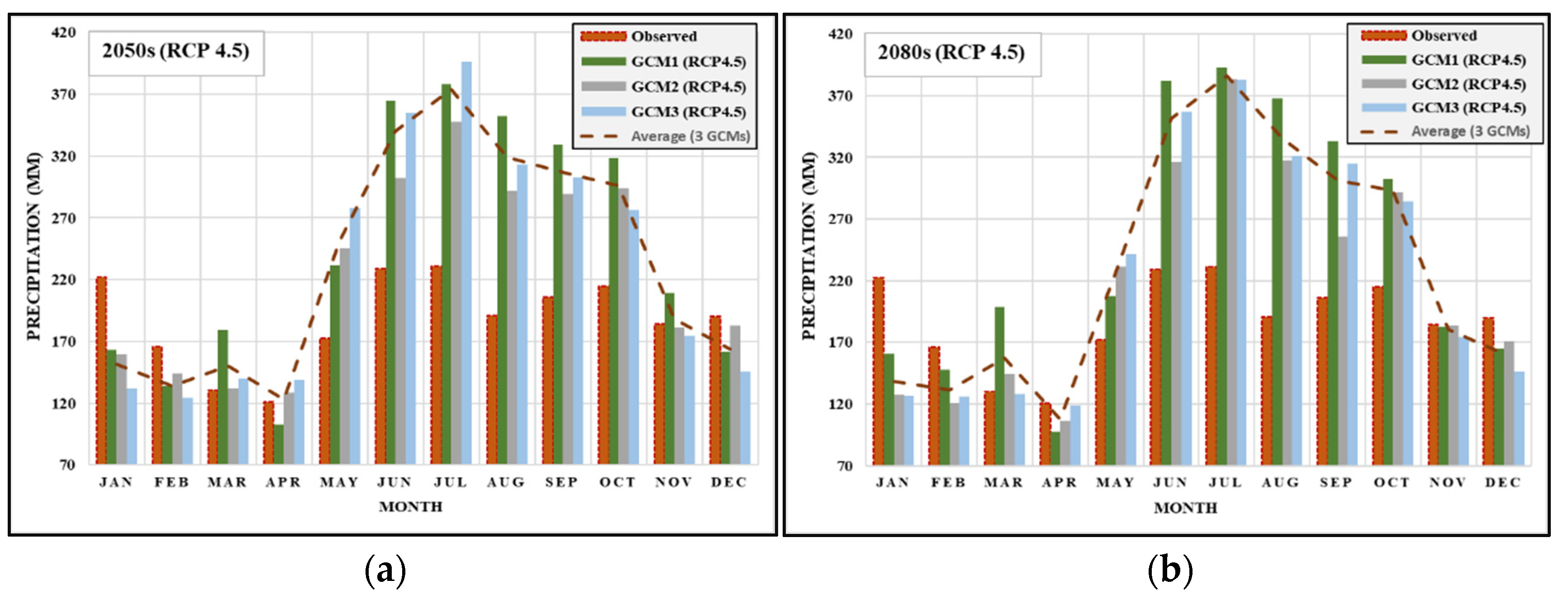
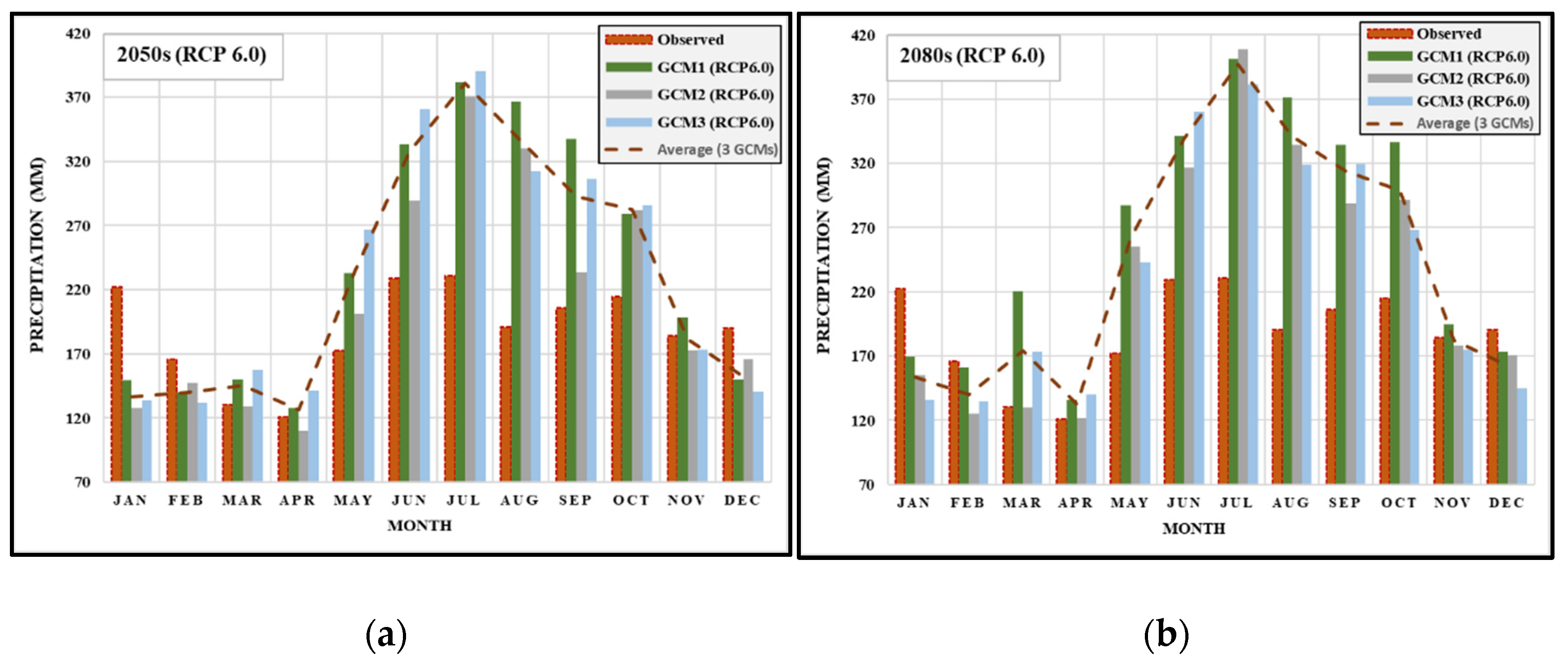
3.2. Climate Change Impact on Precipitation

A comparison of the average observed monthly precipitation for three GCMs under two emission scenarios for the 2050s and 2080s are shown in Figure 5 and Figure 6. There was a clear indication of a significant increase in the monthly mean precipitation under all scenarios of GCMs. The annual mean precipitation is expected to increase to 34.30%, 32.91%, 31.29%, and 39.10% during the 2050s (RCP 4.5), 2080s (RCP 4.5), 2050s (RCP 6.0), and 2080s (RCP 6.0), respectively. The maximum predicted annual mean precipitation is expected to increase by 50% during the 2080s under GCM1 (RCP 6.0), while a 22.80% increase is expected in the minimum increment during the 2050s under GCM2 (RCP 6.0). Moreover, the projections of all scenarios indicate a remarkable increase in precipitation from May to October, while a decrease in precipitation is expected from November to April. The increase in precipitation will lead to a rise in river discharge, and a high risk of flooding is evident. This result is consistent with the trend observed from the study by Tolentino et al., (2016) [39], with Mindanao predicted to experience an increase in river discharge due to the increase of water availability in the period of 2010–2050.

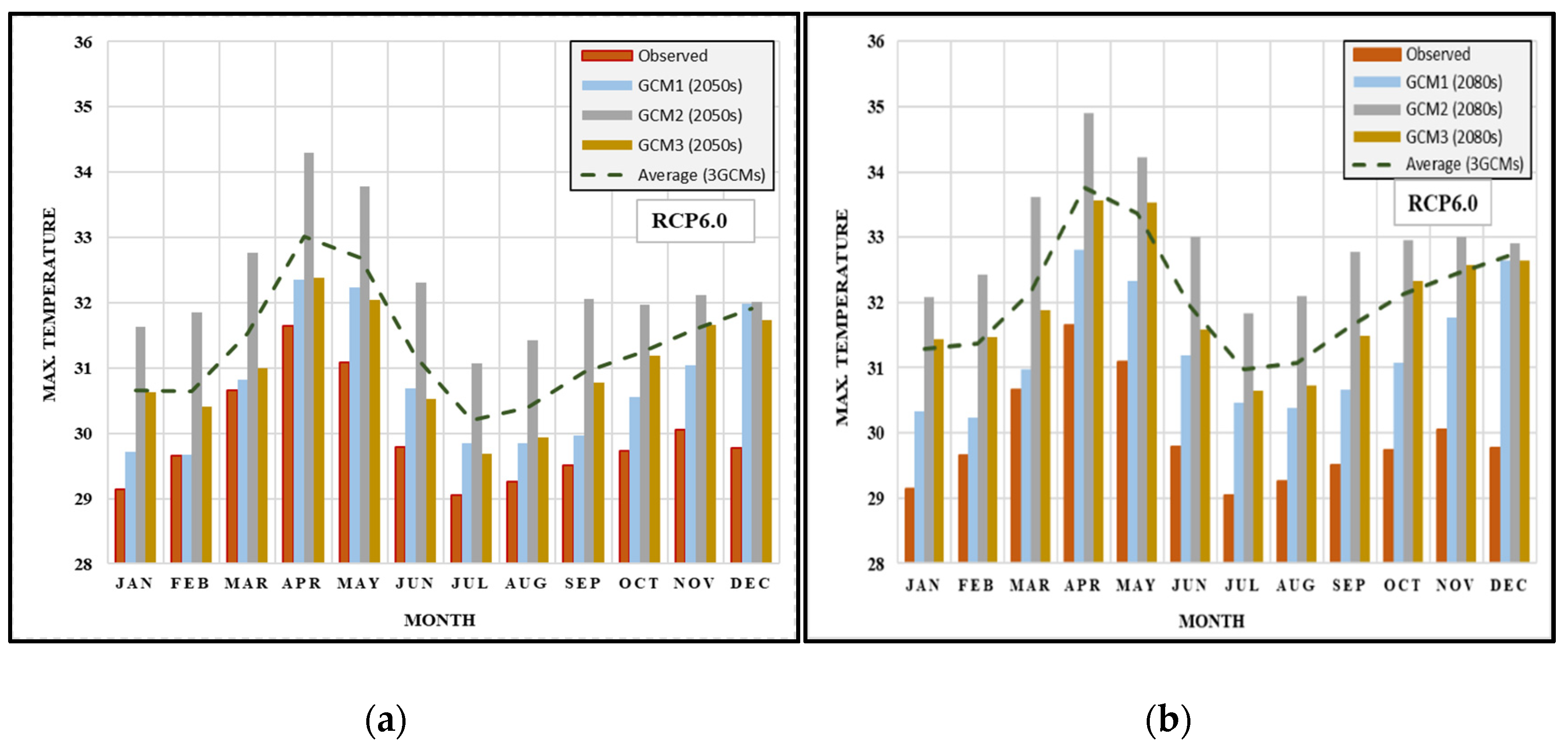
3.3. Climate Change Impact on Maximum Temperature

The extent of change in the monthly variation of projected maximum temperatures under various scenarios and periods is presented in Figure 7 and Figure 8. The maximum temperature increase is 3.04 °C under the GCM2 (RCP6.0) for the timeframe of the 2080s, whereas the smallest increment is 0.78 °C under the GCM1(RCP 6.0) for the period of 2050s. The maximum temperature is expected to rise more in the 2080s than in the 2050s. The monthly maximum mean temperature is expected to increase by 2.09 °C, 2.95 °C, 2.33 °C, and 3.04 °C during 2050s (RCP 4.5), 2080s (RCP 4.5), 2050s (RCP 6.0), and 2080s (RCP 6.0), respectively. In general, all GCMs showed an increase in maximum temperature over the basin. The trend in these results is similar to those in the study of PAGASA (2011), in which the maximum seasonal temperature of Bukidnon and North Cotabato Province was observed to increase in the 2050s projection by 1.6 °C under SRES-B1 (equivalent to RCP 4.5) and by 3.0 °C under SRES-B2 (equivalent to RCP 6.0) [11].

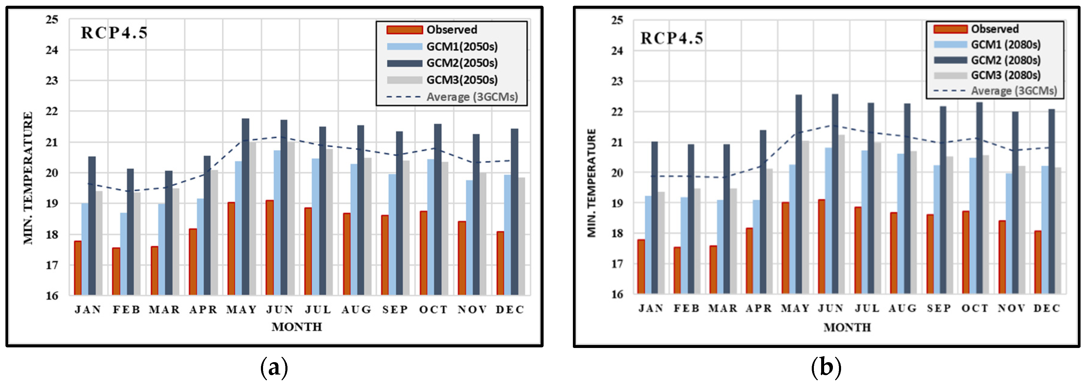
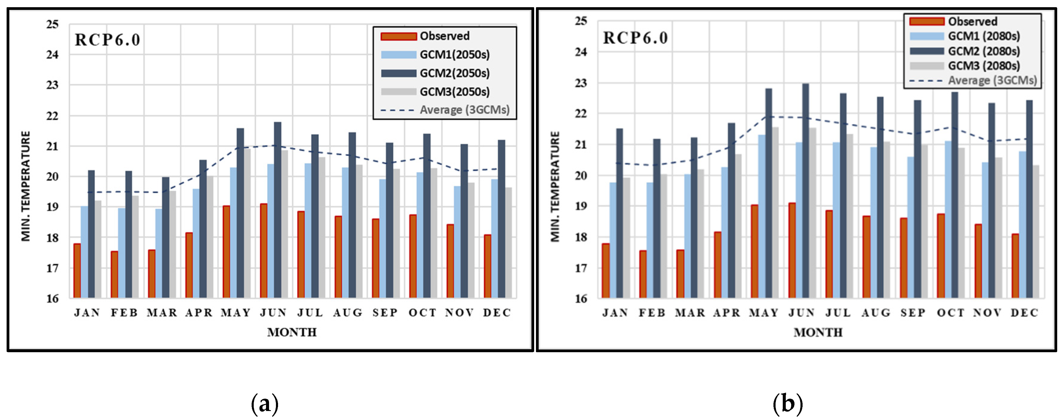
3.4. Climate Change Impact on Minimum Temperature

The monthly average minimum daily temperatures under various scenarios and periods are presented in Figure 9 and Figure 10. The average minimum temperature from 18.4 °C is expected to increase by the highest increment, at 3.83 °C for the timeframe of the 2080s under GCM2 (RCP 6.0). Meanwhile, the smallest increment of change in the minimum temperature is 1.42 °C under the GCM1 (RCP 6.0) of the 2050s. Moreover, the monthly minimum mean temperature is expected to increase by increments of 2.74 °C, 3.50 °C, 2.61 °C, and 3.83 °C during the 2050s (RCP 4.5), 2080s (RCP 4.5), 2050s (RCP 6.0), and 2080s (RCP 6.0), respectively. Evidently, the minimum temperature is expected to rise more in the 2080s timeframe than in the 2050s. Thus, the yearly average of minimum daily temperature showed an increase for all scenarios. The results for the change in minimum temperature are consistent with the findings reported by PAGASA (2011), which found the seasonal minimum temperature of Bukidnon and North Cotabato Province will increase in the 2050s projection by 1.7 °C under SRES-B1 (equivalent to RCP 4.5) and by 2.3 °C under SRES-B2 (equivalent to RCP 6.0) [11].

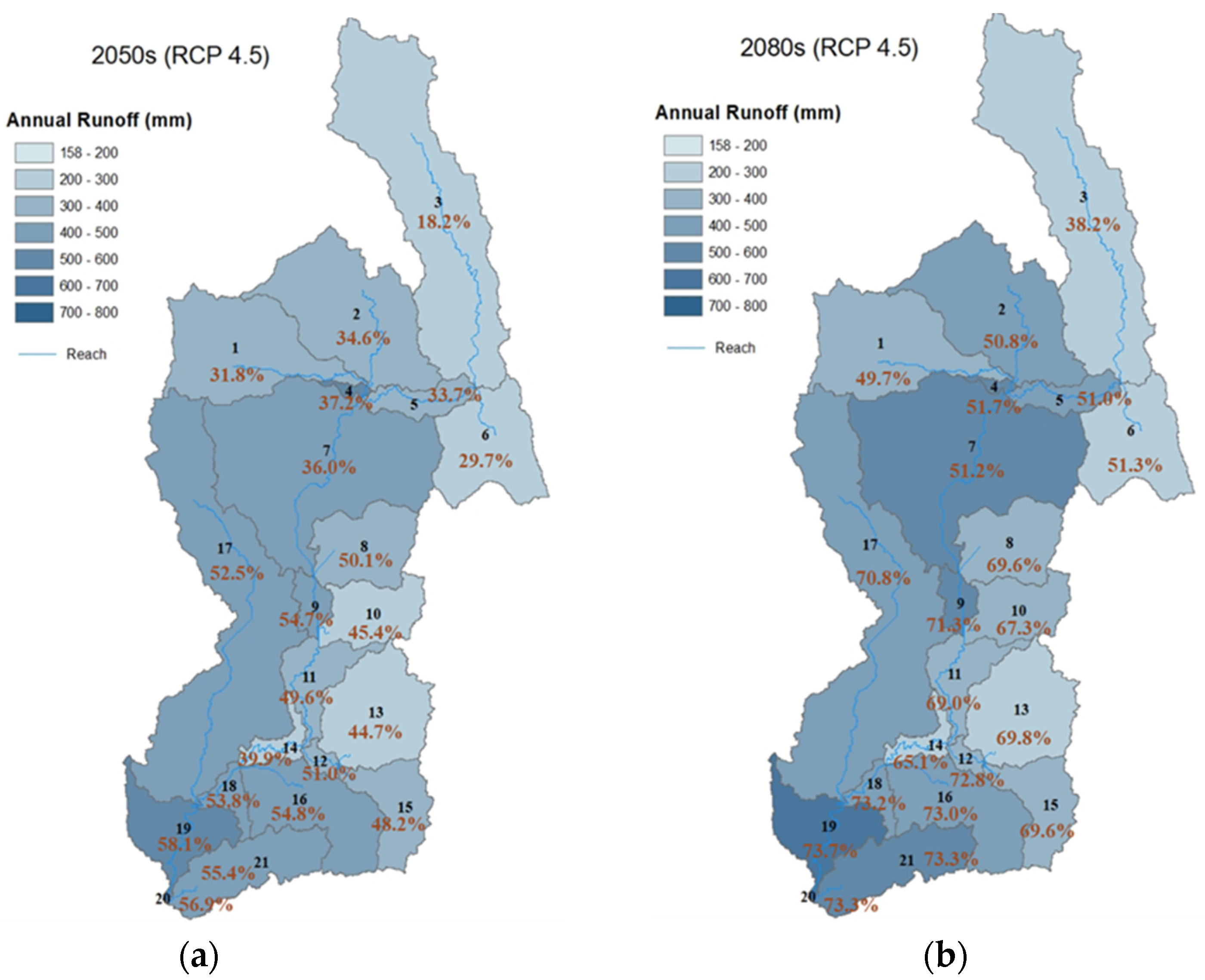
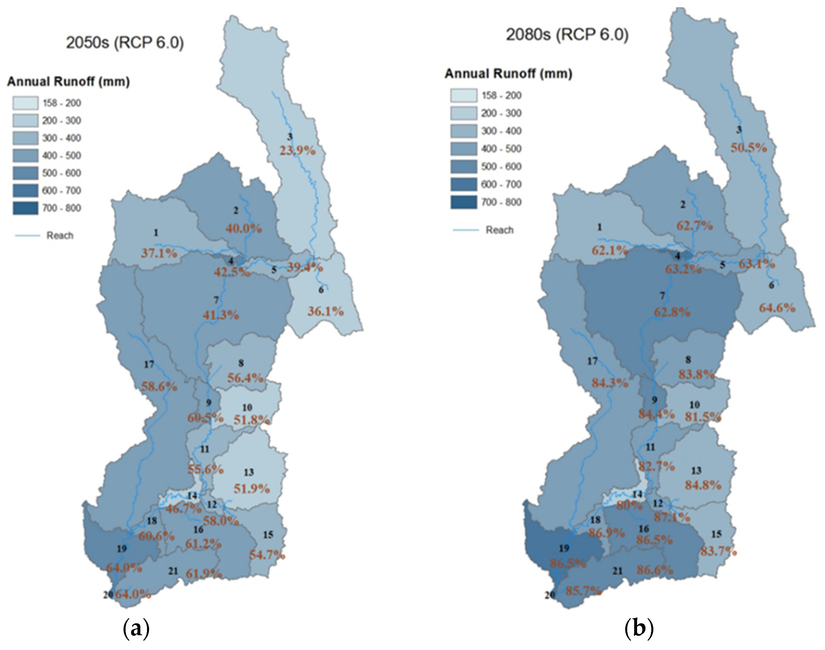
3.5. Impact of Climate Change on Runoff

The annual runoff maps of 21 sub-basins of PRB under RCP 4.5 and 6.0 for all periods are depicted in Figure 11 and Figure 12. The projections showed an increase in annual runoff from 44.58% (equivalent to 377.68 mm) under the RCP 4.5 (2050s) to 76.80% (equivalent to 459.39 mm) under RCP 6.0 (2080s). In the 2050s under RCP 4.5, nine sub-basins (8, 9, 12, 16, 17, 18, 19, 20, 21) will experience an increase in runoff more than 50% larger than that of the baseline period. A higher increase in the runoff is expected in the 2080s under the RCP 4.5 due to the eight sub-basins (9, 12, 16, 17, 18, 19, 20, 21), at more than 70% larger than that of the baseline. In the 2050s under RCP 6.0, six sub-basins (9, 16, 18, 19, 20, 21) will experience increases in runoff more than 60% larger than that of baseline period, while 14 sub-basins were observed to have increases of more than 80% in 2080s under RCP 6.0.

In general, the impact of climate change was clearly shown to be increased in runoff in all sub-basins for all scenarios. It is also important to note that most of these sub-basins affected by the increase in runoff are located in the lower stream of the basin. This indicates a high possibility of frequent flooding in the low-lying areas of Pulangi Basin. Moreover, the highest runoff is observed during the wet season from May to October.

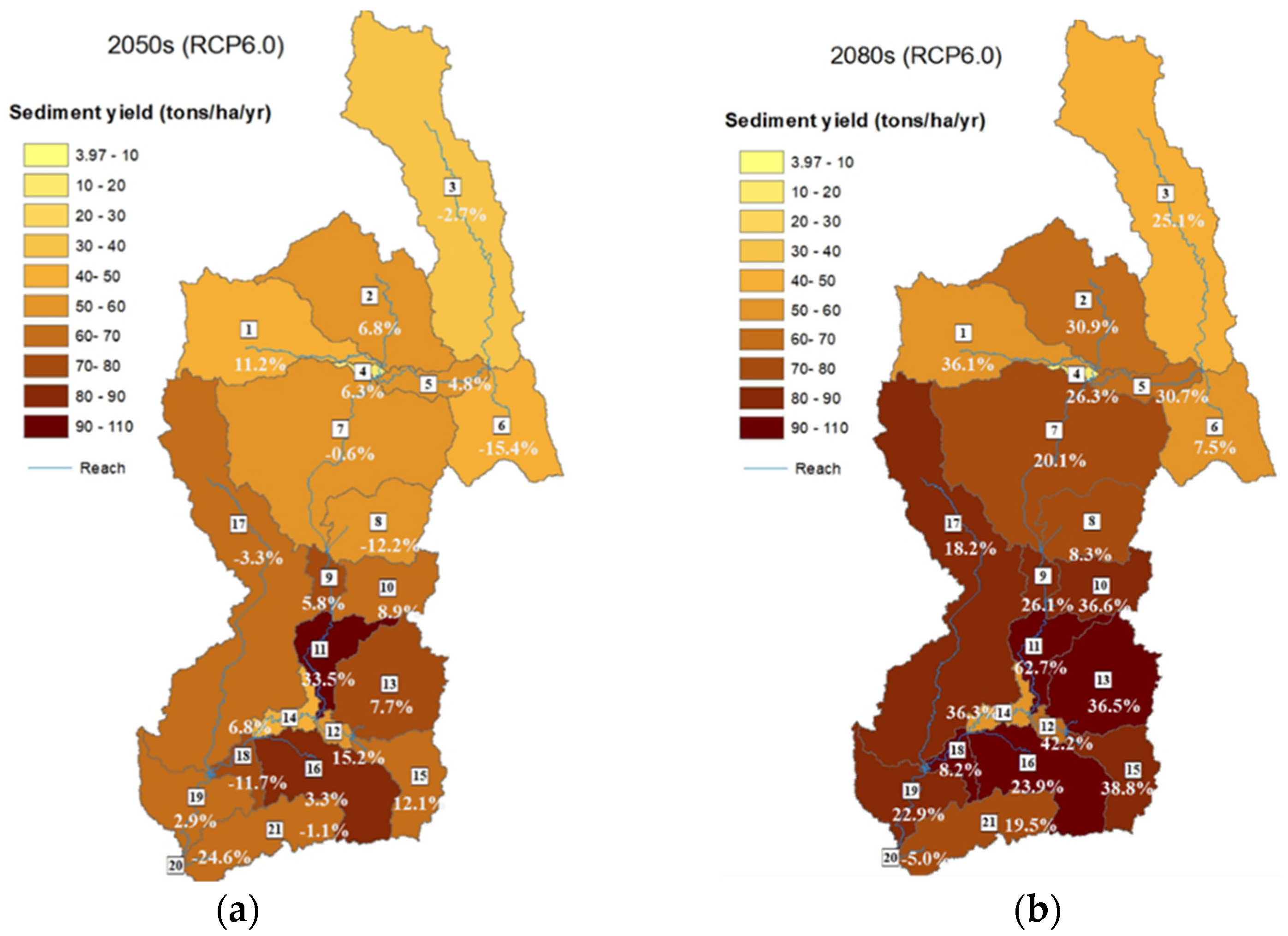
3.6. Impact of Climate Change on Sediment Yield

The changes in sediment yield for the 21 sub-basins of PRB under all scenarios are illustrated in Figure 13 and Figure 14. In all scenarios, an average increase in the annual sediment yield is indicated. Figure 13 and Figure 14 showed that most sub-basins are expected to experience sediment yield and soil erosion, particularly in hilly or mountainous subwatersheds. The sediment yield in the PRB is expected to vary from 1% under GCM1(RCP4.5) of the 2050s to 94.57% under GCM2(RCP6.0) in the 2050s. Moreover, the sediment yield (averaging all sub-basins) is expected to have an average increment of 1.33%, 18.65%, 2.56%, and 26.28% in the scenarios 2050s (RCP 4.5), 2080s (RCP 4.5), 2050s (RCP 6.0), and 2080s (RCP 6.0), respectively. From these results, it can be concluded that the impact of climate change will be greater in terms of the runoff than on sediment yield. These study outcomes indicate that the changes in precipitation and temperature can significantly impact the runoff and sediment yield of the PRB.

Changes in sediment yield may result in extensive changes to the topography in the basin, particularly if they are associated with mudslides after heavy rainfall events. Because runoff inevitably means a loss of soil-nutrients to the water system, this can also result in poorer quality of soils and eutrophication in the watershed, which will cause a series of other problems. Water storage problems can also be expected as a result.

4. Conclusions

The potential impact of climate change on precipitation and temperature was explored in this study, with a focus on the effect on runoff and sediment yield of the Pulangi River Basin (PRB). Future climate changes were projected using the twelve downscaled climate projections from three Global Circulation Models of Couples Model Intercomparison Project Phase 5 under two Representative Concentration Pathways (RCP 4.5 and 6.0) for the 2050s and 2080s and are further compared to the baseline period (1975–2005). SWAT was utilized as a hydrological model to assess climate change.

• While the calibration and validation of data resulted in a satisfactory to good performance in the case of streamflow data, in the case of data for sediment yield, the performance was unsatisafactory. All climate projections indicated a substantial increase in annual precipitation and temperature in all periods under two RCPs, revealing a similar trend for annual runoff and the soil loss rate.
• On a monthly scale, a remarkable increase in precipitation was found for all scenarios from May to October, particularly a southwest monsoon or ‘habagat’ season, and a decrease in rainfall during November to April, especially during in the summer season. These findings suggest a general increased threat of enhanced flooding and excessive soil loss rate, leading to severe erosion and reservoir sedimentation throughout the PRB.
• The large increase in runoff indicated for the lower stream of the basin indicates a high possibility of frequent flooding in the low-lying areas of PRB.
• The excessive soil loss in the PRB, especially in hilly and mountainous regions will result in soil nutrients run-off and water storage problem. Changes can be expected to the silt deposits in low-lying areas, which may be change the topography of the basin.

In this study, the process of overcoming the challenges of using a scientific-based approach to improve water resources in PRB are illustrated. The climate change impact in the PRB was investigated despite the limited amount of data available for the study area. The study methods demonstrate the application of various scientific tools to minimize the effect of uncertainty and improve the model results, and they can be used in other river basins with limited data availability. The model results achieved by this process have the potential to support policymakers when considering the future scenarios in the PRB in efforts to lessen the negative impact of climate change. In future studies, land-use change scenarios and dynamic downscaling climate scenarios (ex. CORDEX Southeast Asia) should be incorporated in model simulation in order to develop better climate change adaptation and mitigation strategies.

References

1. IPCC. Climate Change 2014: Synthesis Report. Contribution of Working Groups I, II and III to the Fifth Assessment Report of the Intergovernmental Panel on Climate Change; Core Writing Team, Pachauri, R.K., Meyer, L.A., Eds.; IPCC: Geneva, Switzerland, 2014.
2. Nguyen, T.T.; Nakatsugawa, M.; Yamada, T.J.; Hoshino, T. Assessing climate change impacts on extreme rainfall and severe flooding during the summer monsoon season in the Ishikari River basin, Japan. Hydrol. Res. Lett. 2020, 14, 155–161. [Google Scholar] [CrossRef]
3. Azari, M.; Moradi, H.R.; Saghafian, B. Climate change impacts on streamflow and sediment yield in the North of Iran. Hydrol. Sci. J. 2016, 61, 123–133. [Google Scholar] [CrossRef]
4. Mehan, S.; Kannan, N.; Neupane, R.P.; McDaniel, R.; Kumar, S. Climate change impacts on the hydrological processes of a small agricultural watershed. Climate 2016, 4, 56. [Google Scholar] [CrossRef]
5. Sangmanee, C.; Wattayakorn, G.; Sojisuporn, P. Simulating changes in discharge and suspended sediment loads of the Bangpakong River, Thailand, driven by future. Maejo Int. J. Sci. Technol. 2013, 7, 72–84. [Google Scholar]
6. Khoi, D.N.; Suetsugi, T. Hydrologic response to climate change: A case study for the Be River Catchment, Vietnam. J. Water Clim. Chang. 2012, 3, 207–224. [Google Scholar] [CrossRef]
7. Tan, M.L.; Ibrahim, A.L.; Yusop, Z.; Chua, V.P.; Chan, N.W. Climate change impacts under CMIP5 RCP scenarios on water resources of the Kelantan River Basin, Malaysia. Atmos. Res. 2017, 189, 1–10. [Google Scholar] [CrossRef]
8. Principe, J.; Blanco, A. Swat Model for Assessment of Climate Change and Land Use / Land Cover Change Impact on Philippine Soil Loss and Exploration of Land Cover-Based Mitigation Measures: Case of Cagayan. ASEAN Eng. J. Part C 2013, 3, 104. [Google Scholar]
9. Alejo, L.A.; Ella, V.B. Assessing the impacts of climate change on dependable flow and potential irrigable area using the swat model. The case of maasin river watershed in Laguna, Philippines. J. Agric. Eng. 2019, 50, 88–98. [Google Scholar] [CrossRef]
10. Arceo, M.G.A.S.; Cruz, R.V.O.; Tiburan, C.L.; Balatibat, J.B.; Alibuyog, N.R. Modeling the hydrologic responses to land cover and climate changes of selected watersheds in the Philippines using soil and water assessment tool (SWAT) model. DLSU Bus. Econ. Rev. 2018, 28, 84–101. [Google Scholar]
11. PAGASA. Climate Change in the Philippines. Philippine Atmospheric, Geophysical and Astronomical Services Administration. 2011; pp. 14–21. Available online: https://dilg.gov.ph/PDF_File/reports_resources/DILG-Resources-2012130-2ef223f591.pdf (accessed on 3 September 2020).
12. Shahin, M. Runoff and Riverflow: Water Resources and Hydrometeorology of the Arab Region; Springer: Dordrecht, The Netherlands, 2007; Volume 59. [Google Scholar]
13. National Power Corporation. Master Plan for the Eleven (11) NPC-Managed Watersheds; National Power Corporation: Quezon City, Philippines, 2015. [Google Scholar]
14. Nippon Koei Co. The Study for Restoration and Upgrading Dams under Operation in the Republic of the Philippines. 2019. Available online: https://www.meti.go.jp/meti_lib/report/H30FY/000156.pdf (accessed on 3 September 2020).
15. Delgado, V.M., Jr. The Effectiveness of Desilting the Pulangi IV Hydropower Plant’s Reservoir. In Proceedings of the 18th Conference of the Electric Power Supply Industry (CEPSI 2010) in Taipei International Convention Center, Taipei, Taiwan, 24–28 October 2010. [Google Scholar]
16. Dessai, S.; Lu, X.; Risbey, J.S. On the role of climate scenarios for adaptation planning. Glob. Environ. Chang. 2005, 15, 87–97. [Google Scholar] [CrossRef]
17. Santoso, H.; Idinoba, M.; Imbach, P. Climate Scenarios: What we need to know and how to gernerate them. Work. Pap. 2008, 45, 25. [Google Scholar]
18. Neitsch, S.; Arnold, J.; Kiniry, J.; Williams, J. Soil and Water Assessment Tool Theoretical Documentation Version 2009; Texas Water Resources Institute: College Station, TX, USA, 2011. [Google Scholar] [CrossRef]
19. Paringit, E.C.; Puno, G.R. LiDAR Surveys and Flood Mapping of Upper Pulangi River; University of the Philippines Training Center for Applied Geodesy and Photogrammetry: Quezon City, Philippines, 2017. [Google Scholar]
20. van Vuuren, D.P.; Edmonds, J.; Kainuma, M.; Riahi, K.; Thomson, A.; Hibbard, K.; Hurtt, G.C.; Kram, T.; Krey, V.; Lamarque, J.F.; et al. The representative concentration pathways: An overview. Clim. Chang. 2011, 109, 5–31. [Google Scholar] [CrossRef]
21. Guiamel, I.A.; Lee, H.S. Watershed modelling of the mindanao river basin in the philippines using the SWAT for water resource management. Civ. Eng. J. 2020, 6, 626–648. [Google Scholar] [CrossRef] [Green Version]
22. Marin, R.A.; Jamis, C.V. Soil erosion status of the three sub-watersheds in Bukidnon Province, Philippines. Adv. Environ. Sci. 2017, 8, 194–204. [Google Scholar]
23. Moriasi, D.N.; Arnold, J.G.; van Liew, M.W.; Bingner, R.L.; Harmel, R.D.; Veith, T.L. Model Evaluation Guidelines for Systematic Quantification of Accuracy in Watershed Simulations. Trans. ASABE 2007, 50, 885–900. [Google Scholar] [CrossRef]
24. Brighenti, T.M.; Bonumá, N.B.; Grison, F.; de A. Mota, A.; Kobiyama, M.; Chaffe, P.L.B. Two calibration methods for modeling streamflow and suspended sediment with the swat model. Ecol. Eng. 2019, 127, 103–113. [Google Scholar] [CrossRef]
25. Gupta, H.V.; Sorooshian, S.; Yapo, P.O. Status of Automatic Calibration for Hydrologic Models: Comparison with Multilevel Expert Calibration. J. Hydrol. Eng. 1999, 4, 135–143. [Google Scholar] [CrossRef]
26. Nash, J.E.; Sutcliffe, J.V. River flow forecasting through conceptual models part I—A discussion of principles. J. Hydrol. 1970, 10, 282–290. [Google Scholar] [CrossRef]
27. Schaefli, B.; Gupta, H.V. Do Nash values have value? Hydrol. Process. 2007, 21, 2075–2080. [Google Scholar] [CrossRef] [Green Version]
28. Santhi, C.; Arnold, J.G.; Williams, J.R.; Dugas, W.A.; Srinivasan, R.; Hauck, L.M. Validation of the SWAT model on a large river basin with point and nonpoint source. J. Am. Water Resour. Assoc. 2001, 37, 1169–1188. [Google Scholar] [CrossRef]
29. Liu, D. A rational performance criterion for hydrological model. J. Hydrol. 2020, 590, 125488. [Google Scholar] [CrossRef]
30. Legates, D.R.; McCabe, G.J. Evaluating the use of “goodness-of-fit” measures in hydrologic and hydroclimatic model validation. Water Resour. Res. 1999, 35, 233–241. [Google Scholar] [CrossRef]
31. Arnold, J.G.; Srinivasan, R.; Muttiah, R.S.; Williams, J.R. Large Area Hydrologic Modeling and Assessment Part I: Model Development. J. Am. Water Resour. Assoc. 1998, 34, 73–89. [Google Scholar] [CrossRef]
32. Williams, J.R.; Berndt, H.D. Sediment Yield Prediction Based on Watershed Hydrology. Trans. Am. Soc. Agric. Eng. 1977, 20, 1100–1104. [Google Scholar] [CrossRef]
33. Vaghefi, S.A.; Abbaspour, N.; Kamali, B.; Abbaspour, K.C. A toolkit for climate change analysis and pattern recognition for extreme weather conditions—Case study: California-Baja California Peninsula. Environ. Model. Softw. 2017, 96, 181–198. [Google Scholar] [CrossRef]
34. Chen, J.; Brissette, F.P.; Leconte, R. Uncertainty of downscaling method in quantifying the impact of climate change on hydrology. J. Hydrol. 2011, 401, 190–202. [Google Scholar] [CrossRef]
35. Lu, G.Y.; Wong, D.W. An adaptive inverse-distance weighting spatial interpolation technique. Comput. Geosci. 2008, 34, 1044–1055. [Google Scholar] [CrossRef]
36. Abbaspour, K.C.; Yang, J.; Maximov, I.; Siber, R.; Bogner, K.; Mieleitner, J.; Zobrist, J.; Srinivasan, R. Modelling hydrology and water quality in the pre-alpine/alpine Thur watershed using SWAT. J. Hydrol. 2007, 333, 413–430. [Google Scholar] [CrossRef]
37. Abbaspour, C.K. SWAT Calibration and Uncertainty Program (SWAT-CUP)—A User Manual; EAWAG, Swiss Federal Institute of Aquatic Science and Technology: Zurich, Switzerland, 2015. [Google Scholar]
38. Sahu, M.; Lahari, S.; Gosain, A.K.; Ohri, A. Hydrological Modeling of Mahi Basin Using SWAT. J. Water Resour. Hydraul. Eng. 2016, 5, 68–79. [Google Scholar] [CrossRef]
39. Tolentino, P.L.M.; Poortinga, A.; Kanamaru, H.; Keesstra, S.; Maroulis, J.; David, C.P.C.; Ritsema, C.J. Projected impact of climate change on hydrological regimes in the Philippines. PLoS ONE 2016, 11, 1–14. [Google Scholar] [CrossRef] [PubMed] [Green Version]
Figure 1. The procedure developed in the study.
Sustainability 13 09041 g001
Figure 2. Location of the Pulangi River Basin and its 21 sub-basins.
Sustainability 13 09041 g002
Figure 3. The map of PRB’s (a) digital elevation model, (b) land use/land cover map, (c) soil classification map, (d) land slope.
Sustainability 13 09041 g003
Figure 4. A comparison of monthly observed and simulated streamflow for calibration and validation with monthly rainfall data.
Sustainability 13 09041 g004
Figure 5. A comparison of the averaged observed monthly precipitation for three GCMs under RCP 4.5 for the periods (a) 2050s and (b) 2080s.
Sustainability 13 09041 g005
Figure 6. A comparison of the averaged observed monthly precipitation for three GCMs under RCP 6.0 for the periods (a) 2050s and (b) 2080s.
Sustainability 13 09041 g006
Figure 7. A comparison of the monthly maximum temperature of three GCMs under RCP 4.5 for the periods (a) 2050s and (b) 2080s.
Sustainability 13 09041 g007
Figure 8. A comparison of the monthly maximum temperature of three GCMs under RCP 6.0 for the periods (a) 2050s and (b) 2080s.
Sustainability 13 09041 g008
Figure 9. A comparison of the monthly minimum temperature of three GCMs under RCP 4.5 for the periods (a) 2050s and (b) 2080s.
Sustainability 13 09041 g009
Figure 10. A comparison of the monthly minimum temperature of three GCMs under RCP 6.0 for the periods (a) 2050s and (b) 2080s.
Sustainability 13 09041 g010
Figure 11. The annual runoff map of the 21 sub-basins of PRB for the periods (a) 2050s and (b) 2080s under RCP 4.5 emission scenario.
Sustainability 13 09041 g011
Figure 12. The annual runoff map of the 21 sub-basins of PRB for the periods (a) 2050s and (b) 2080s under RCP 6.0 emission scenario.
Sustainability 13 09041 g012
Figure 13. The sediment yield map of 21 sub-basins of PRB for the periods (a) 2050s and (b) 2080s under RCP 4.5 emission scenario.
Sustainability 13 09041 g013
Figure 14. The sediment yield map of 21 sub-basins of PRB for the periods (a) 2050s and (b) 2080s under the RCP 6.0 emission scenario.
Sustainability 13 09041 g014