Demand Forecasting for Liquified Natural Gas Bunkering by Country and Region Using Meta-Analysis and Artificial Intelligence

Abstract

Ship exhaust emission is the main cause of coastal air pollution, leading to premature death from cardiovascular cancer and lung cancer. In light of public health and climate change concerns, the International Maritime Organization (IMO) and several governments are reinforcing policies to use clean ship fuels. In January 2020, the IMO reduced the acceptable sulfur content in ship fuel to 0.5% m/m (mass/mass) for sustainability. The use of liquified natural gas (LNG) as a ship fuel is currently the most likely measure to meet this regulation, and LNG bunkering infrastructure investment and network planning are underway worldwide. Therefore, the aim of this study is to predict the LNG bunkering demand for investment and planning. So far, however, there has been little quantitative analysis of LNG bunkering demand prediction. In this study, first, the global LNG bunkering demand was predicted using meta-regression analysis. Global demand for LNG bunkering is forecast to increase from 16.6 million tons in 2025 to 53.2 million tons in 2040. Second, LNG bunkering prediction by country and region was performed through analogy and artificial intelligence methods. The information and insights gained from this study may facilitate policy implementation and investments.

1. Introduction

Ship exhaust emission is at the root of coastal air pollution [1]. Over 70% of shipping emissions can be detected up to 400 km inshore [2]. In the past, particulate matter 2.5 emissions from ships, which cause cardiovascular cancer and lung cancer, have resulted in as many as 64,000 annual deaths [3]. In this context, keeping in mind public health and environmental protection concerns, the International Maritime Organization (IMO) has strengthened ship exhaust gas regulations [4].

The issue of air pollution by ships was first discussed in 1973, when the International Convention for the Prevention of Pollution from Ships (MARPOL 73/78) was adopted [5]. In 1997, the MARPOL Diplomatic Conference, which investigated ships’ carbon dioxide emissions as part of preparing an inventory of such emissions at a global level, adopted Resolution 8 to explore the issue of air pollution caused by ships in the context of climate change. It is important to note that the international community showed an understanding of the relevance of ship exhaust emissions to climate change. MARPOL Annex VI was implemented as an environmental regulation in 2005. With effect from January 2020, the IMO Marine Environment Protection Committee has reduced the accpetable sulfur content in ship fuel to 0.5% m/m [6,7,8].

The IMO has also presented policy goals regulating greenhouse gas emissions. Based on the 2008 figures, the goal is to reduce emissions by half by 2050 and to zero by 2100 [9]. Several governments are implementing these policies. The European Union (EU) has made carbon neutrality by 2050 as a top priority, and South Korea has declared that the country will achieve complete carbon neutrality by 2050.

In the past, numerous industry policies prioritizing the environment have been implemented. However, at present, the dichotomy between industrial and environmental benefits is not acceptable. The paradigm shift in the international community, which is known as sustainability, is leading to changes in the behavior of industries. For instance, Totalenergies is looking for business opportunities by linking LNG as a ship fuel to achieve the IMO’s decarbonisation target [10], and DNV-GL, which accounts for 43% of LNG-fuelled ships [11], is very optimistic about the LNG demand forecast compared to other forecasting agencies [9,12,13,14,15,16,17,18]. In addition, it is believed that the problem of methane slip caused by the use of LNG ship fuels will soon be resolved [19].

There are three kinds of measures for international shipping companies: the use of LSFO, scrubber installation, and the use of LNG. In comparison to diesel, LNG can reduce sulfur emissions by 99–100%, nitrogen oxides by 80–95%, and particulate matter by 90–99% as well as limiting carbon dioxide emissions to less than 20% [6,20,21,22,23,24,25,26]. For the other two options, LSFO’s production capacity is insufficient. With LSFO there is still the need for treatment of nitrate oxides and greenhouse gases, and it is 30% more expensive than heavy fuel oil [5,6]. Whereas, scrubbers are expensive to install and difficult to apply to small vessels [6]. Comparatively, therefore, LNG is the most beneficial [6,8,27].

For accurate LNG bunkering market growth prediction, it is essential to consider the energy content of each marine fuel [28]. The energy content of heavy fuel oil, marine gas oil and LNG is 40 MJ/kg, 43 MJ/kg, and 48 MJ/kg, respectively [29]. LNG’s energy efficiency is increasing its appeal compared to traditional petroleum fuels [27]. Previous research has shown a rapid decline of heavy fuel oil in marine fuel mix [9,17]. In contrast, LNG trade, which accounted for 28.6% of the natural gas trade in 2000, increased to 45.7% in 2018 [30]. For the reasons mentioned above, it is quite likely that the LNG bunkering industry will grow in the near future.

Peng et al. (2021) conducted a systematic review of existing LNG bunkering studies [6]. These can be classified into five groups: (i) LNG bunkering network planning, (ii) general layout of LNG bunkering stations, (iii) scheme design of LNG bunkering stations, (iv) risk management of LNG bunkering stations, and (v) strategy formulation for LNG promotion in the shipping industry. As demonstrated by these categories, although there has been extensive research on LNG bunkering, quantitative analyses of LNG bunkering demand prediction utilizing detailed methodologies are limited.

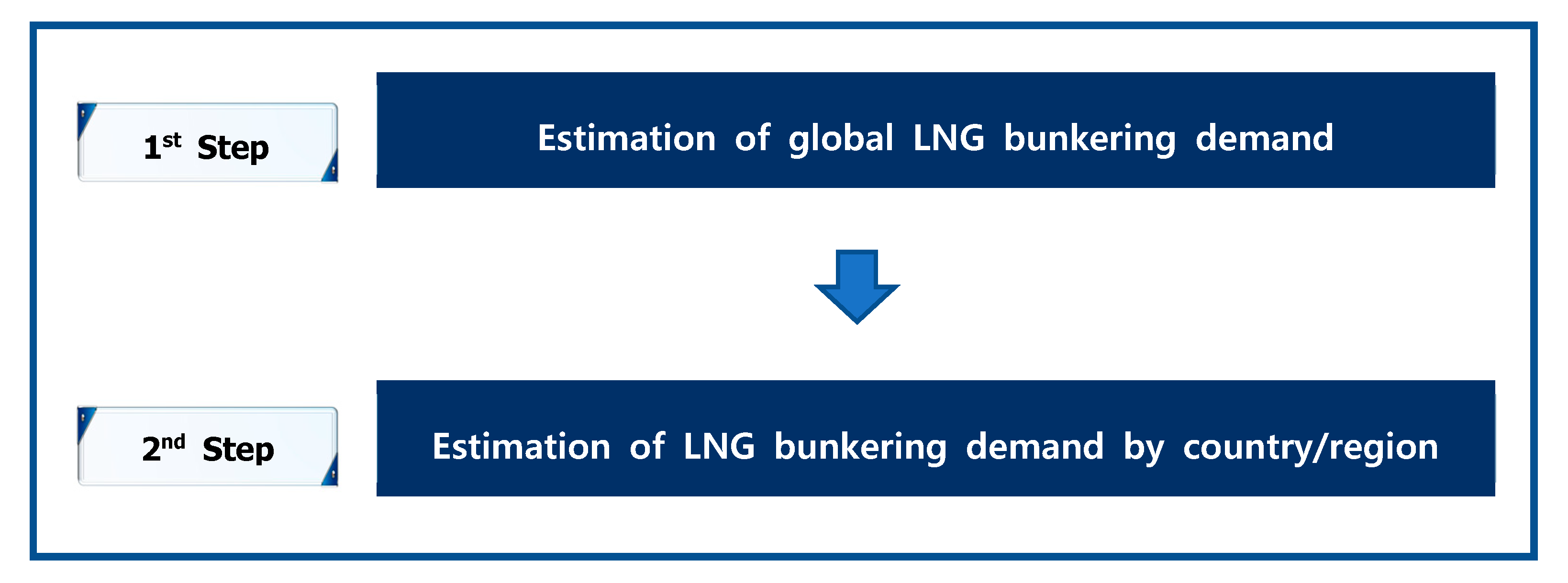
LNG bunkering demand estimation is essential for LNG bunkering network planning, scheme design of LNG bunkering stations, and developing industry revitalization strategies [6]. What is important in global bunkering network planning is detailed country-wise demand forecasts [6]. Thus, an objective of this study was to investigate global LNG bunkering demand prediction and forecast LNG bunkering demand by country and region. Previous studies on demand forecasts regarding LNG bunkering have been mainly conducted by international organizations and business groups but no forecasting methodology is presented.

In this study, we consider various methodologies, such as meta-regression, analogy, and artificial intelligence, to predict LNG bunkering demand. This investigation takes a top-down approach and makes two contributions as compared to existing studies. First, it reduces the uncertainty present in existing research results. We analyze the relationship between year and LNG demand through the regression model utilizing previous findings. Meta-regression is used to integrate different predictions by agencies. Second, it improves the accuracy of prediction by selecting, out of the five forecasting methods that have been actively used in the field in recent years, the one that is best suited to the study condition in order to secure the scientific soundness.

This study offers LNG demand information that can facilitate the implementation of environmental policies by governments and investment decision making by industries. LNG demand forecasting is needed to verify the feasibility of the sub-policy measures of international organizations and governments to address climate change. It is also important for LNG infrastructure investment decisions such as the selection of LNG-powered ships and building facilities of LNG bunkering terminals.

The remaining part of the paper proceeds as follows. Section 2 presents an overview of the relevant literature. Section 3 presents methodologies for estimating LNG bunkering demand. Section 4 present the LNG bunkering demand outlook. Section 5 concludes this study and offers policy implications.

2. Literature Review

2.1. Status of Global LNG Bunkering

The huge population and fast economic growth of non-OECD regions of Asia, including India and China, predict the expansion of the energy consumption market in Asia. In particular, China is pursuing an energy transition from coal to gas, which is linked to future LNG demand [31]. The United States is focusing on cost-competitive development in shallow gas and is expected to grow into a potential exporter on the level of Qatar or Australia [11].

Investment in LNG bunkering is increasing globally, with the EU, China, Singapore, South Korea, Japan, and North America showing particular interest. The EU already operates 50 LNG bunkering stations, with 13 more under construction [32]. Norway, Sweden, Belgium, Germany, and the Netherlands are centers of the EU’s LNG bunkering industry [33]. Peng et al.’s (2021) review, which focused on Chinese studies pertaining to the country’s potential application of inland LNG bunkering since 2010, reported the construction or conversion of 300 LNG propulsion vessels used inland [6]. China built more than 10 bunkering stations in 2019 and is pursuing a strategy to expand inland to the coast. Furthermore, Chinese companies have performed research and development (R&D) activities in LNG fuel supply technology with government support [6]. The Port of Singapore is striving to become a central hub for the Asian LNG market [6]. In South Korea, there is a plan for the Ministry of Oceans and Fisheries (MOF) to build an LNG bunkering station at Busan Port [12]. Japan, the world’s largest importer of LNG, is trying to become an international LNG bunkering hub [34]. Overall, Asian countries are in intense competition to become the major LNG bunkering players in the region. The United States is building an LNG bunkering station at Jacksonville in Florida, and in Canada, the federal government and the government of British Columbia are working together to promote an LNG bunkering station in Western Canada [6].

It is necessary to increase the number of LNG-powered ships to expand the market for this fuel. However, there is no consensus among agencies on the exact number of LNG vessels in operation. According to Peng et al. (2021), the total number in 2020 was 175 [6]. DNV-GL (2019) counted 172 ships in operation in 2019 [13], with the numbers as of 2018 and 2017 standing at 121 [14] and 112 [12], respectively. Despite this lack of clarity, it cannot be denied that the operation of LNG vessels is in the nascent stage and that their number will gradually increase [6,12,13,14].

The importance of LNG as a ship fuel is increasing, and R&D in this area is being actively conducted because of the IMO’s environmental regulations and the demand for large LNG-powered ships. Existing LNG vessels are generally small and medium-sized tugboats, passenger ships, and cruise ships. Within a few years, however, owing to rapid technological development, LNG-powered ships will likely increase in size and ships of all types are expected to adopt LNG fuel [6].

2.2. Previous Research on LNG Bunkering Demand Forecasting

As mentioned above, there has been little quantitative analysis of LNG bunkering demand forecasting not only because the use of LNG as a ship fuel is in the nascent stage but also because the number of LNG propulsion ships compared to the total number of ships is relatively small [6]. However, in China, where LNG is receiving significant national attention, several demand forecasting studies have been conducted. Wang predicted LNG demand considering relevant policies, port throughput, and fuel consumption [35,36]. Yang (2016) presented a formula for predicting LNG demand based on gray-system prediction theory and port throughput [37]. Liu (2020) reported a demand forecasting method considering macro market demand, demand for specific LNG bunkering projects, and factors influencing demand [38]. The MOF (2018) also conducted a global and national LNG bunkering demand forecast [12]. Global demand was estimated by considering the size of LNG propulsion ships and annual LNG consumption according to ship model. For the forecast of demand by country, panel data on oil bunkering processing volume were utilized with the scenarios presented by obtaining a forecast of oil bunkering proportion in each country and multiplying it by the global LNG bunkering demand. Oil bunkering is the entire process of supplying fuels such as bunker-C oil and diesel oil to ships [12]. Park and Park (2019) derived the daily LNG bunkering requirements of Busan Port through simulation by considering the gross tonnage and LNG fuel consumption of each ship model [8].

Former LNG bunkering demand forecasts, performed by international organizations and business groups, were derived considering volatility of oil prices and the number of LNG-powered ships in a scenario or performed iteratively. The LNG bunkering demand predictions vary widely from one forecasting agency to another. It is likely that the assumptions, methodologies, and competence of practitioners differ by agency. Prediction is a statement of future values of variables such as demand. In other words, predictions about the future may vary depending on a predictor’s perspective and environmental conditions at the time of forecasting. Therefore, demand estimation could be inherently variable and should be repeated.

3. Methodology and Data

3.1. Forecasting Method: Top-Down Approach

Previous studies in the energy field have utilized either a top-down or bottom-up approach [39]. The top-down approach makes predictions at the top level, subsequently calculating the prediction values according to the proportions of the components [39]. The bottom-up approach, on the contrary, predicts each component and then aggregates the values to make an overall prediction [40]. To increase prediction accuracy, several studies have combined these two methods or compared the findings from each technique [41,42,43,44,45]. The top-down method is a logical and practical approach when the entire dataset is available, while the bottom-up method is an appropriate choice when the data for each component are available [39]. In this study, the top-down approach was utilized because of the availablity of data pertaining to global LNG bunkering demand. As shown in Figure 1, we estimated global LNG bunkering demand and then predicted LNG bunkering demand by country and region.

3.2. Global LNG Bunkering Demand Forecast

The analysis of global LNG bunkering demand was based on the results of ten studies (

Table 1. Results of global liquified natural gas bunkering demand from previous studies (unit: 1000 tons).

	2025	2030	2035	2040	2045	2050
IHS (2020) [15]	19,300	31,200	45,700	65,700	80,400	81,700
IEA New Policy (2019) [16]	7800	15,800	25,100	37,000	-	-
DNV-GL (2019) [9]	23,850	44,687	65,542	78,712	-	-
S&P Global Platts (2019) [17]	19,375	27,396	-	-	-	-
The Ministry of Oceans and Fisheries in South Korea (2018) [12]	12,925	14,712	24,462	24,269	-	-
IHS (2017) [13]	16,500	27,600	43,900	70,000	-	-
IEA New Policy (2017) [14]	23,900	29,700	36,200	41,300	-	-
Lloyds Register (2017) [14]	19,000	25,000	30,000	42,500	-	-
PWC (2017) [14]	-	27,000	-	-	-	-
Gazprom (2012) [18]	27,789	33,643	-	-	-	-

The data is adopted from [9,12,13,14,15,16,17,18].

). Most data were reported by international organizations and business groups. A weighting assessing the quality of data may be taken into account for demand forecasting of global LNG bunkering. However, because it is difficult to determine which data is more reliable, the data are analyzed by meta-regression. Meta-regression is a method of performing regression analysis using quantified information from prior studies. It facilitates the synthesis of findings from previous studies investigating similar research questions [46].

Equation (1) is the formula for the estimate of global LNG bunkering demand. The dependent variable is the global demand for LNG bunkering in the marine sector, and the independent variable $Time$ is the year. We used Time as a proxy variable. According to Moore’s law, time can be a represented technological progress [47]. As a similar example, the use of time as a proxy variable can be found in economics. For instance, time was used as a proxy variable for technological indicators to understand the relationship between productivity growth and technology improvement [48].

In this study, the independent variable $Time$ was assumed to include the volume of goods transported by ships, the number of LNG-powered ships, the level of LNG bunkering infrastructure, and the number of aging ships. Because these variables will increase over time. $Deman{d}_{i,t}$ is the estimated value of global LNG demand for t-time of the $i$th previous study. Regarding $Time$, numbers were used in place of years to derive appropriate results from the regression equation. For example, the year 2020 was replaced by 1; therefore, the year 2040 was substituted by 21. The residual term is ${\epsilon }_{i,t}$.

$$Deman{d}_{i,t}={\beta }_{0,i}+{\beta }_{1}TIME+{\epsilon }_{i,t}$$

(1)

Considering the sensitivity of the demand forecast, it proceeded in three scenarios: Scenario 1 (most likely), Scenario 2 (the industry friendly), and Scenario 3 (the environmentally friendly). Scenario 2 used the fifth percentile of the $Time$ coefficient in the derived regression equation. Scenario 3 utilized the 95th percentile of the $Time$ coefficient in the regression equation. The constant applied to Scenarios 1, 2 and 3 was derived from the regression equation.

3.3. LNG Bunkering Demand Estimation by Country and Region

The analogy method was used for the estimation of LNG bunkering demand by country and region. As mentioned previously, the LNG bunkering market is in the early stage; therefore, historical data are limited. Accordingly, future demand for new products is predicted through comparative analogy with the demand patterns or supply situations of similar products, or with cases in developed countries. In this study, the similar product was oil bunkering, which is the only possible comparison for LNG bunkering in the energy sector.

Therefore, this study assumes that the per-country proportion of oil bunkering and the proportion of LNG bunkering will be identical in the future. Liquified natural gas bunkering ratios for each country and region were derived from oil bunkering forecasts. It was assumed that the LNG bunkering ratios of each country and region would be equivalent to the oil bunkering ratios from 2021 to 2040.

Equation (2) is the prediction model for demand by country and region. The dependent variable is oil bunkering by country and region. The independent variable is the quantity of goods transported by country and region. Country and region were used as dummy variables, and included South Korea, China, Hong Kong, Japan, the rest of Asia, Singapore, the EU, Africa, the Middle East, the Americas, and the rest of the world. Time is expressed as t. $Trad{e}_{i,t}$ means the volume of goods transported by ships in the area $i$ in year t. The residual term is ${\epsilon }_{i,t}$.

$$OilBun{k}_{i,t}={\beta }_{0i}+{\beta }_{1}Trad{e}_{i,t}+{\epsilon }_{i,t}$$

(2)

The data used in the analysis is presented in Table 2 and Table 3. Table 2 shows oil bunkering performance from 2000 to 2014. We utilized data in Table 3 for oil bunkering forecasting from 2015 to 2030.

The analysis utilized five models: generalized linear model (GLM), deep learning, random forest, gradient boosting decision tree (GBDT), and support vector machine (SVM). The LNG bunkering demand by country and region was predicted by selecting the model with the best forecasting performance. The basic concepts are described.

3.3.1. Generalized Linear Model (GLM)

Nelder et al. (1972) proposed GLM as an extended linear regression model [49]. It is used when the categorical variable is the dependent variable or when it is difficult to assume that the dependent variable follows a normal distribution. Namely, GLM is used when regression analysis or analysis of variance cannot be applied. The model assumes a linear relationship between the independent variable and the functional value of ${\mu }_i$. ${\mu }_i$ is the expected value of the dependent variable $y_i$.

Equation (3) shows the basic GLM formula. Equation (4) describes the logarithmic function or exponential function of GLM.

$$g \left({\mu }_i\right)=x_i^{\prime }\beta$$

(3)

$$\ln \left(\mu \right)={\beta }_0+{\beta }_1{x}_1+{\beta }_2{x}_2+\dots +{\beta }_p{x}_p \mu =e^{{\beta }_0+{\beta }_1{x}_1+{\beta }_2{x}_2+\dots +{\beta }_p{x}_p}$$

(4)

3.3.2. Deep Learning

Machine learning is a subfield of artificial intelligence that is used to develop algorithms that enable computers to learn. The categories of machine learning are supervised, unsupervised, and reinforcement learning.

Artificial neural networks, a type of machine learning, imitate the human brain. Deep learning is based on artificial neural networks [50]. It mimics how human brain cells receive input signals and deliver messages to other neurons to make decisions [51]. The deeper the neural network, the better the performance that can result, and this depth dramatically improves performance compared to traditional machine learning [50]. Neural networks consist of input layers, hidden layers, and output layers. The hidden layer usually comes to a conclusion after two steps. Equation (5) displays the analysis of the first step, which calculates the summation of the input value, weights, and bias. The weight is w_i and the input parameter is x_i. The second step is to run neurons using the sigmoid function to output a value between 0 and 1 [51].

$$y={\displaystyle \sum }_{i=1}^{n}w{x}_i+bias$$

(5)

$$Sigmoid=1/\left(1+e^{-y}\right)$$

(6)

The loss is calculated by Equation (7). The actual result and predicted result are $y$ and y¹, respectively. As the neural network trains, the predicted value approaches the actual value [51].

$$loss={\left(y-y^1\right)}^2$$

(7)

In summary, deep learning extracts key features in complex and large amounts of data through a combination of several nonlinear transformation techniques.

3.3.3. Random Forest

The random forest is a type of ensemble learning method that aggregates multiple decision trees (classification of regression) to create a final prediction model [52]. The final classification decision is made after k rounds of training [53]. Categorical classification problems are determined by majority voting, whereas regression problem is determined by the mean value.

$$H\left(x\right)=arg\underset{Y}{max}{\sum }_{i=1}^{k}I\left(h_i\left(x\right)=Y\right)$$

(8)

H(x) means the combined classification model. h_i represents the classification results of a single decision tree. $Y$ means the output target variable. $I$(•) is an indicative function [53].

$$V=\left(A-A_1\right)/OOB$$

(9)

The importance of variables is obtained by Equation (9). A is the number of samples correctly classified before replacement. A₁ is the number of samples correctly classified after substitution [53]. About a third of the bootstrap training set data are not used in the model [54]. These discarded data are called out-of-bag data (OOB), which are used as verification data again. Therefore, out-of-bag data enhance the model’s strength [54].

3.3.4. Gradient Boosting Decision Tree (GBDT)

The GBDT model is a powerful machine learning method that can perform regression or classification analysis [55]. It utilizes a combination of models with weak predictive power to enhance the overall predictive power [55]. The decision tree model is mainly used for GBDT. GBDT consist of three stages.

Stage 1: Creation of a consistently decreasing loss function [56]. N is a sample set, $\gamma$ is a constant in Equation (10).

$$f_0\left(x\right)=argmi{n}_{\gamma } {\displaystyle \sum }_{i=1}^{N}L\left(y_i, \gamma \right)$$

(10)

Stage 2: Repetition of the following four steps:

Step 1: To estimate the residuals, the negative gradient value of the loss function is calculated and applied [56].

$${\gamma }_{im}=-{\left[\partial L\left(y_i,f\left(x_i\right)\right)/\partial f\left(x_i\right)\right]}_{f=f_m-1}$$

(11)

Step 2: The value corresponding to the leaf node of the regression tree is calculated [56].

Step 3: A linear search is performed to estimate the leaf node region and reduce loss function [56].

$${\gamma }_{jm}=argmi{n}_{\gamma }{\displaystyle \sum }_{x_i\in R_{jm}}L\left(y_i,f_{m-1}\left(x_i\right)+\gamma \right)$$

(12)

Step 4: The regression tree is updated by Equation (13) [56].

$$f_m\left(x\right)=f_{m-1}\left(x\right)+{\displaystyle \sum }_{j=1}^{J_m}{\gamma }_{jm}I\left(x\in R_{jm}\right)$$

(13)

Stage 3: The final GBDT is output as a function of x as shown in Equation (14) [56].

$$f\left(x\right)=f_M\left(x\right)$$

(14)

3.3.5. Support Vector Machine (SVM)

The support vector machine, a type of machine learning, is a supervised learning model for pattern recognition and data analysis. This is mainly used for classification and regression.

An SVM is initially provided a dataset with data from two categories. The SVM algorithm determines the category for new data based on a given dataset. It is performed by a non-probabilistic binary linear classification model. The created classification model is expressed as a boundary in the space where the data are mapped, and the SVM algorithm finds the boundary with the largest width among them [57].

Linear SVMs express predictors in two dimensions. If $y_i$ belong to either category, it can be expressed as +1 and vice versa as −1 [57]. The straight line is called a separating plane.

$$y=+1\mathrm{if}ax+b\ge 0\mathrm{or}-1\mathrm{if}ax+b<0$$

(15)

By extending this formula, we can express the plane of the p-dimensional image. ${\beta }_i$ is the coefficient of plane [57].

$${\beta }_0+{\beta }_1{x}_1+{\beta }_2{x}_2+\dots +{\beta }_p{x}_p=0$$

(16)

All data can be classified by Equation (17).

$$f={\beta }_0+{\beta }_1{x}_1+{\beta }_2{x}_2+\dots +{\beta }_p{x}_p={\tilde{x}}^T·\tilde{\beta }+{\beta }_0$$

(17)

The SVM classifier is derived by Equation (18). ${\epsilon }_i$ means the classification error of the ith point. C means the sum of the classification errors of all data [57]. C is determined by the researcher. For a detailed process of estimating $\tilde{\beta }$, refer to [57].

$$\begin{array}{c}\mathrm{maximize}M\\ {\beta }_0, {\beta }_1, \dots , {\beta }_p, {\epsilon }_1, {\epsilon }_2, \dots ,{\epsilon }_p\\ \mathrm{subject}\mathrm{to}\\ {\displaystyle {\displaystyle \sum }_{j=1}^p}{\beta }_j^2=1\\ y_i\left({\beta }_0+{\beta }_1{x}_{i1}+{\beta }_2{x}_{i2}+\dots +{\beta }_p{x}_{ip}\right)\ge M\left(1-{\epsilon }_i\right)\\ {\epsilon }_i\ge 0, {\displaystyle {\displaystyle \sum }_{i=1}^n}{\epsilon }_i\le C\end{array}$$

(18)

Table 2. Reported quantity of oil bunkering from country/region (unit: 1000 tons).

	South Korea	China	Hong Kong	Japan	Rest of Asia	Singapore	EU	Africa	The Middle East	The Americas
2000	8503	2487	2056	4971	6548	17,096	35,082	6145	13,082	32,274
2001	8253	2659	2666	4360	7475	18,427	36,519	5716	12,224	24,051
2002	7988	2965	2929	4580	7165	18,156	38,043	5347	11,687	28,382
2003	8656	3069	3036	5012	8159	19,308	39,785	6331	13,342	24,616
2004	9004	3970	4485	5260	9042	22,060	42,773	6285	15,153	28,916
2005	9165	4729	4152	5889	9689	23,933	43,880	6400	16,278	31,535
2006	9234	5476	5091	5546	12,240	26,814	47,053	6021	17,902	33,599
2007	8466	6422	6281	5431	15,456	30,023	49,676	6323	19,340	36,576
2008	8110	6519	5738	5059	18,282	33,387	50,132	6190	21,609	36,716
2009	7388	6767	6634	4509	21,411	34,792	44,136	5648	18,663	32,991
2010	7931	8259	9166	4451	23,985	39,248	43,682	5471	20,340	14,713
2011	7743	8723	6924	3949	24,740	41,577	44,142	5203	21,531	33,256
2012	7562	8590	7125	3886	25,230	41,229	40,454	5678	21,734	27,961
2013	7367	7462	7537	3731	27,157	41,306	37,899	4991	23,275	27,638
2014	7444	6939	6290	3371	27,893	41,104	36,105	4129	24,213	23,580

Source: International Energy Agency [58], re-cited by the Ministry of Oceans and Fisheries in South Korea (2018). Note: “Rest of Asia” refer to the continent of Asia excluding South Korea, China, Hong Kong, Japan and Singapore.

Table 2. Reported quantity of oil bunkering from country/region (unit: 1000 tons).

	South Korea	China	Hong Kong	Japan	Rest of Asia	Singapore	EU	Africa	The Middle East	The Americas
2000	8503	2487	2056	4971	6548	17,096	35,082	6145	13,082	32,274
2001	8253	2659	2666	4360	7475	18,427	36,519	5716	12,224	24,051
2002	7988	2965	2929	4580	7165	18,156	38,043	5347	11,687	28,382
2003	8656	3069	3036	5012	8159	19,308	39,785	6331	13,342	24,616
2004	9004	3970	4485	5260	9042	22,060	42,773	6285	15,153	28,916
2005	9165	4729	4152	5889	9689	23,933	43,880	6400	16,278	31,535
2006	9234	5476	5091	5546	12,240	26,814	47,053	6021	17,902	33,599
2007	8466	6422	6281	5431	15,456	30,023	49,676	6323	19,340	36,576
2008	8110	6519	5738	5059	18,282	33,387	50,132	6190	21,609	36,716
2009	7388	6767	6634	4509	21,411	34,792	44,136	5648	18,663	32,991
2010	7931	8259	9166	4451	23,985	39,248	43,682	5471	20,340	14,713
2011	7743	8723	6924	3949	24,740	41,577	44,142	5203	21,531	33,256
2012	7562	8590	7125	3886	25,230	41,229	40,454	5678	21,734	27,961
2013	7367	7462	7537	3731	27,157	41,306	37,899	4991	23,275	27,638
2014	7444	6939	6290	3371	27,893	41,104	36,105	4129	24,213	23,580

Source: International Energy Agency [58], re-cited by the Ministry of Oceans and Fisheries in South Korea (2018). Note: “Rest of Asia” refer to the continent of Asia excluding South Korea, China, Hong Kong, Japan and Singapore.

Table 3. Total Cargo volume processing performance by ship for country/region (unit: 1000 tons).

Year	South Korea	China	Hong Kong	Japan	Rest of Asia	Singapore	EU	Africa	The Middle East	The Americas	Worldwide
2000	340,517	288,867	56,291	799,523	717,770	104,268	861,799	227,127	215,468	1,275,363	5,394,134
2001	344,764	337,265	54,439	774,791	691,235	104,986	857,670	237,301	228,436	1,276,760	5,339,925
2002	360,726	396,850	53,079	764,473	727,507	108,570	787,626	239,404	230,029	1,263,472	5,410,777
2003	372,500	506,678	55,379	792,037	762,575	102,346	856,988	236,577	245,727	1,325,131	5,749,881
2004	395,719	618,864	55,679	805,846	852,201	112,880	897,423	263,505	265,178	1,410,237	6,288,936
2005	400,667	733,645	59,769	815,376	939,965	116,878	929,822	282,003	315,045	1,508,340	6,624,967
2006	410,596	807,688	61,675	815,281	911,709	122,822	973,707	299,802	324,954	1,538,150	6,885,326
2007	430,134	935,292	53,967	824,282	947,731	130,571	1,004,958	335,903	347,296	1,466,477	7,155,373
2008	458,618	1,018,817	54,421	836,720	1,009,879	142,490	1,012,010	352,135	404,096	1,486,855	7,635,620
2009	439,053	1,433,016	55,293	701,891	1,040,674	153,936	779,672	367,069	341,549	1,246,578	7,093,793
2010	496,120	1,572,775	55,286	790,417	1,329,114	158,460	889,912	406,564	416,669	1,385,424	8,074,668
2011	530,953	1,777,014	57,753	780,924	1,394,575	170,289	910,193	405,340	398,894	1,427,554	8,591,036
2012	534,640	1,938,858	57,011	805,069	1,377,204	177,931	894,209	439,562	417,698	1,363,774	8,680,149
2013	539,477	2,217,053	59,080	815,433	1,446,673	178,904	869,190	459,435	413,071	1,295,170	8,941,593
2014	554,301	2,199,561	66,850	798,048	1,542,311	196,943	864,599	477,839	438,348	1,352,232	9,089,621
2015	571,759	2,246,444	61,508	781,350	1,576,759	186,331	905,996	465,853	438,988	1,299,161	9,122,179
2016	596,314	2,393,992	60,487	768,020	1,620,377	186,548	878,465	463,451	455,982	1,289,368	9,305,834
2017	609,526	2,565,298	61,211	778,236	1,687,100	186,947	914,123	484,377	469,126	1,342,990	9,699,876
2018	628,276	2,628,827	61,835	808,266	1,754,104	189,318	933,963	507,925	486,802	1,368,274	9,974,955
2019	642,680	2,693,121	62,990	854,805	1,823,627	192,458	962,731	532,587	505,043	1,397,809	10,284,991
2020	656,166	2,787,692	64,915	841,537	1,920,064	196,446	1,003,414	564,983	524,598	1,423,205	10,615,013
2021	666,102	2,866,064	66,763	861,726	2,020,105	200,531	1,032,020	594,475	542,562	1,446,149	10,941,056
2022	676,803	2,944,158	68,252	875,250	2,127,185	204,863	1,057,613	623,224	560,742	1,470,589	11,262,813
2023	690,310	3,050,165	69,749	888,334	2,237,002	209,911	1,080,546	652,682	577,489	1,497,749	11,615,415
2024	704,319	3,168,999	71,060	899,995	2,335,055	214,917	1,102,733	682,374	593,780	1,526,479	11,967,222
2025	717,899	3,305,854	72,059	910,382	2,431,351	219,731	1,125,292	712,542	610,323	1,557,083	12,335,142
2026	730,430	3,455,634	72,928	919,397	2,525,754	224,238	1,146,377	742,264	626,774	1,586,062	12,708,146
2027	743,609	3,611,294	73,771	928,747	2,620,726	228,542	1,167,141	771,893	641,437	1,617,720	13,088,608
2028	757,808	3,748,782	74,542	939,388	2,713,065	232,963	1,190,000	802,298	656,078	1,651,112	13,456,220
2029	772,193	3,877,786	75,380	951,877	2,807,770	237,298	1,214,230	833,709	672,240	1,685,165	13,823,987
2030	785,807	3,979,991	76,362	966,112	2,907,828	241,615	1,241,179	866,155	689,194	1,720,028	14,177,463

Note: Data from 2000 to 2016 are by reported results and data from 2017 to 2030 are by forecast results. Source: The Ministry of Oceans and Fisheries in South Korea (2018).

Table 3. Total Cargo volume processing performance by ship for country/region (unit: 1000 tons).

Year	South Korea	China	Hong Kong	Japan	Rest of Asia	Singapore	EU	Africa	The Middle East	The Americas	Worldwide
2000	340,517	288,867	56,291	799,523	717,770	104,268	861,799	227,127	215,468	1,275,363	5,394,134
2001	344,764	337,265	54,439	774,791	691,235	104,986	857,670	237,301	228,436	1,276,760	5,339,925
2002	360,726	396,850	53,079	764,473	727,507	108,570	787,626	239,404	230,029	1,263,472	5,410,777
2003	372,500	506,678	55,379	792,037	762,575	102,346	856,988	236,577	245,727	1,325,131	5,749,881
2004	395,719	618,864	55,679	805,846	852,201	112,880	897,423	263,505	265,178	1,410,237	6,288,936
2005	400,667	733,645	59,769	815,376	939,965	116,878	929,822	282,003	315,045	1,508,340	6,624,967
2006	410,596	807,688	61,675	815,281	911,709	122,822	973,707	299,802	324,954	1,538,150	6,885,326
2007	430,134	935,292	53,967	824,282	947,731	130,571	1,004,958	335,903	347,296	1,466,477	7,155,373
2008	458,618	1,018,817	54,421	836,720	1,009,879	142,490	1,012,010	352,135	404,096	1,486,855	7,635,620
2009	439,053	1,433,016	55,293	701,891	1,040,674	153,936	779,672	367,069	341,549	1,246,578	7,093,793
2010	496,120	1,572,775	55,286	790,417	1,329,114	158,460	889,912	406,564	416,669	1,385,424	8,074,668
2011	530,953	1,777,014	57,753	780,924	1,394,575	170,289	910,193	405,340	398,894	1,427,554	8,591,036
2012	534,640	1,938,858	57,011	805,069	1,377,204	177,931	894,209	439,562	417,698	1,363,774	8,680,149
2013	539,477	2,217,053	59,080	815,433	1,446,673	178,904	869,190	459,435	413,071	1,295,170	8,941,593
2014	554,301	2,199,561	66,850	798,048	1,542,311	196,943	864,599	477,839	438,348	1,352,232	9,089,621
2015	571,759	2,246,444	61,508	781,350	1,576,759	186,331	905,996	465,853	438,988	1,299,161	9,122,179
2016	596,314	2,393,992	60,487	768,020	1,620,377	186,548	878,465	463,451	455,982	1,289,368	9,305,834
2017	609,526	2,565,298	61,211	778,236	1,687,100	186,947	914,123	484,377	469,126	1,342,990	9,699,876
2018	628,276	2,628,827	61,835	808,266	1,754,104	189,318	933,963	507,925	486,802	1,368,274	9,974,955
2019	642,680	2,693,121	62,990	854,805	1,823,627	192,458	962,731	532,587	505,043	1,397,809	10,284,991
2020	656,166	2,787,692	64,915	841,537	1,920,064	196,446	1,003,414	564,983	524,598	1,423,205	10,615,013
2021	666,102	2,866,064	66,763	861,726	2,020,105	200,531	1,032,020	594,475	542,562	1,446,149	10,941,056
2022	676,803	2,944,158	68,252	875,250	2,127,185	204,863	1,057,613	623,224	560,742	1,470,589	11,262,813
2023	690,310	3,050,165	69,749	888,334	2,237,002	209,911	1,080,546	652,682	577,489	1,497,749	11,615,415
2024	704,319	3,168,999	71,060	899,995	2,335,055	214,917	1,102,733	682,374	593,780	1,526,479	11,967,222
2025	717,899	3,305,854	72,059	910,382	2,431,351	219,731	1,125,292	712,542	610,323	1,557,083	12,335,142
2026	730,430	3,455,634	72,928	919,397	2,525,754	224,238	1,146,377	742,264	626,774	1,586,062	12,708,146
2027	743,609	3,611,294	73,771	928,747	2,620,726	228,542	1,167,141	771,893	641,437	1,617,720	13,088,608
2028	757,808	3,748,782	74,542	939,388	2,713,065	232,963	1,190,000	802,298	656,078	1,651,112	13,456,220
2029	772,193	3,877,786	75,380	951,877	2,807,770	237,298	1,214,230	833,709	672,240	1,685,165	13,823,987
2030	785,807	3,979,991	76,362	966,112	2,907,828	241,615	1,241,179	866,155	689,194	1,720,028	14,177,463

Note: Data from 2000 to 2016 are by reported results and data from 2017 to 2030 are by forecast results. Source: The Ministry of Oceans and Fisheries in South Korea (2018).

In five models, input variables are the quantity of goods transported by country and region, as well as a region-specific dummy variable. Output variable is oil bunkering by country and region.

4. Results

4.1. Global LNG Bunkering Demand Forecast

Table 4. Results of meta-regression.

	Coefficient	Standard Error	t-Statistics	p-Value	5th Percentile	95th Percentile
Constant	2026.13	4875.41	0.41	0.68	−7892.97	11,945.23
Time	2434.89 *	321.48	7.57	0.00	1780.85	3088.94
R-squared		0.6348
Adjusted R2		0.6237
Standard error		12,313.55
Number of observations		35

* Statistically significant at α = 0.01.

shows the statistical results of the global LNG bunkering demand forecast. The global LNG bunkering demand forecast model (Equation (1)) has the coefficient of determination of 0.63. The constant was not statistically significant. The coefficient of the independent variable $Time$ was significantly estimated at the 1% level.

We utilized the regression equation derived from the meta-regression analysis to predict demand. Figure 2 presents the results of the three scenarios. According to the Scenario 1, the most likely, global demand for LNG bunkering is expected to reach 6.9 million tons in 2021, 16.6 million tons in 2025, 28.8 million tons in 2030, 41.0 million tons in 2035, and 53.2 million tons in 2040. Scenario 2, the industry friendly scenario, predicted demand to reach 8.2 million tons in 2021, 20.6 million tons in 2025, 36.0 million tons in 2030, 51.5 million tons in 2035, and 66.9 million tons in 2040. Scenario 3, the environmentally friendly scenario, predicted demand to reach to 5.6 million tons in 2021, 12.7 million tons in 2025, 21.6 million tons in 2030, 30.5 million tons in 2035, and 39.4 million tons in 2040.

4.2. LNG Bunkering Demand Estimation by Country and Region

We analyzed five forecasting models. Forecasting error rate is measured as the out-of-sample performance with one-step-ahead forecast. As measure of forecasting accuracy, the mean absolute percentage error (MAPE) are used widely in the following manner:

$$\frac{{\sum }_{t=1}^L\frac{\left|y_t-{\widehat{y}}_t\right|}{y_t}}{L}\times 100$$

(19)

where $y_t$ and ${\widehat{y}}_t$ are actual data and forecasts for L periods.

The MAPE results obtained from the error rate of each prediction model are shown in

Table 5. Error rates of prediction models.

Model	MAPE
Generalized linear model	20.00%
Deep learning	17.53%
Random forest	27.45%
Gradient boosting decision trees	37.47%
Support vector machine	32.68%

Note: The best MAPE is shown in bold.

. The MAPE is the indicator to assess the effectiveness of the model [59]. The smaller the values of metrics, the better the forecasting performance of the model [59]. The deep learning model had the highest goodness of fit and was selected because of its reliability. We utilized the RapidMiner 9.9 statistical package for data analysis.

The result of deep learning analysis is shown in Figure 3. The horizontal axis is the actual value and the vertical axis is the prediction. The root mean square error value was 5482.4316. In Figure 3, the red dotted line indicates that the actual and predicted values were completely coincident. The results of the estimates were concentrated around the red dotted line; hence, the actual and predicted values are very similar.

Table 6. Share of oil bunkering forecast by country and region (unit: 1000 tons).

	South Korea		China		Hong Kong		Japan		Rest of Asia		Singapore		EU		Africa		The Middle East		The Americas
2015	13,708	5.48%	20,901	8.35%	12,495	4.99%	6840	2.73%	29,475	11.78%	38,160	15.25%	42,989	17.18%	18,029	7.20%	31,005	12.39%	36,646	14.64%
2016	13,941	5.53%	22,466	8.90%	12,482	4.95%	6694	2.65%	30,142	11.95%	38,163	15.12%	42,737	16.94%	18,011	7.14%	31,098	12.32%	36,591	14.50%
2017	14,066	5.49%	24,289	9.48%	12,492	4.87%	6806	2.66%	31,163	12.16%	38,168	14.89%	43,064	16.80%	18,167	7.09%	31,175	12.16%	36,893	14.40%
2018	14,244	5.50%	24,976	9.64%	12,500	4.82%	7134	2.75%	32,189	12.42%	38,197	14.74%	43,246	16.69%	18,344	7.08%	31,283	12.07%	37,035	14.29%
2019	14,381	5.48%	25,671	9.79%	12,515	4.77%	7644	2.91%	33,253	12.68%	38,236	14.58%	43,510	16.59%	18,528	7.06%	31,396	11.97%	37,201	14.18%
2020	14,509	5.46%	26,694	10.04%	12,541	4.72%	7499	2.82%	34,729	13.07%	38,286	14.41%	43,884	16.51%	18,770	7.06%	31,516	11.86%	37,344	14.05%
2021	14,604	5.42%	27,541	10.23%	12,566	4.67%	7720	2.87%	36,260	13.47%	38,337	14.24%	44,146	16.40%	18,991	7.05%	31,627	11.75%	37,473	13.92%
2022	14,705	5.39%	28,433	10.42%	12,586	4.61%	7868	2.88%	37,899	13.89%	38,391	14.07%	44,381	16.27%	19,206	7.04%	31,738	11.63%	37,611	13.79%
2023	14,833	5.36%	29,650	10.71%	12,606	4.55%	8011	2.89%	39,580	14.30%	38,454	13.89%	44,592	16.11%	19,427	7.02%	31,841	11.51%	37,764	13.65%
2024	14,966	5.33%	31,057	11.06%	12,623	4.50%	8138	2.90%	41,081	14.64%	38,517	13.72%	44,792	15.96%	19,649	7.00%	31,942	11.38%	37,926	13.51%
2025	15,103	5.30%	32,774	11.50%	12,636	4.44%	8252	2.90%	42,555	14.94%	38,577	13.54%	44,989	15.79%	19,875	6.98%	32,043	11.25%	38,098	13.37%
2026	15,233	5.26%	34,928	12.07%	12,648	4.37%	8358	2.89%	44,000	15.20%	38,633	13.35%	45,173	15.61%	20,097	6.94%	32,145	11.10%	38,261	13.22%
2027	15,386	5.23%	37,166	12.63%	12,659	4.30%	8483	2.88%	45,433	15.44%	38,687	13.15%	45,354	15.42%	20,319	6.91%	32,235	10.96%	38,440	13.07%
2028	15,551	5.21%	39,143	13.11%	12,670	4.24%	8625	2.89%	46,818	15.68%	38,742	12.97%	45,554	15.26%	20,546	6.88%	32,325	10.83%	38,628	12.94%
2029	15,718	5.19%	40,998	13.53%	12,681	4.18%	8792	2.90%	48,238	15.92%	38,796	12.80%	45,766	15.10%	20,781	6.86%	32,425	10.70%	38,819	12.81%
2030	15,876	5.17%	42,467	13.82%	12,694	4.13%	8982	2.92%	49,739	16.19%	38,850	12.65%	45,997	14.97%	21,024	6.84%	32,529	10.59%	39,029	12.71%

provides the forecast of oil bunkering by country and region from 2015 to 2030 using deep learning and data from 2000 to 2014 (Table 2). The share of oil bunkering from 2031 to 2040 was assumed to remain constant from 2030, because the data for cargo volume processing performance is available for forecasting until 2030 (Table 3).

In the EU, oil bunkering is expected to increase from 43.0 to 46.0 million tons. In Singapore, it is anticipated to rise from 38.2 to 38.9 million tons. In the rest of Asia, it is expected to grow from 29.5 to 49.7 million tons. China’s outlook is high: the predicted growth is from 20.9 to 42.5 million tons. In Hong Kong, the forecast is from 12.5 to 12.7 million tons. In the Americas, there is an expected increase from 36.6 to 39.0 million tons. In the Middle East, the anticipated growth is from 31.0 to 32.5 million tons. In Africa, the predicted increase is from 18.0 to 21.0 million tons. In South Korea, the expected increase is from 13.7 to 15.9 million tons. In Japan, the expected rise is from 6.8 to 9.0 million tons.

4.3. LNG Bunkering Demand Forecast by Country and Region Based on the Scenarios

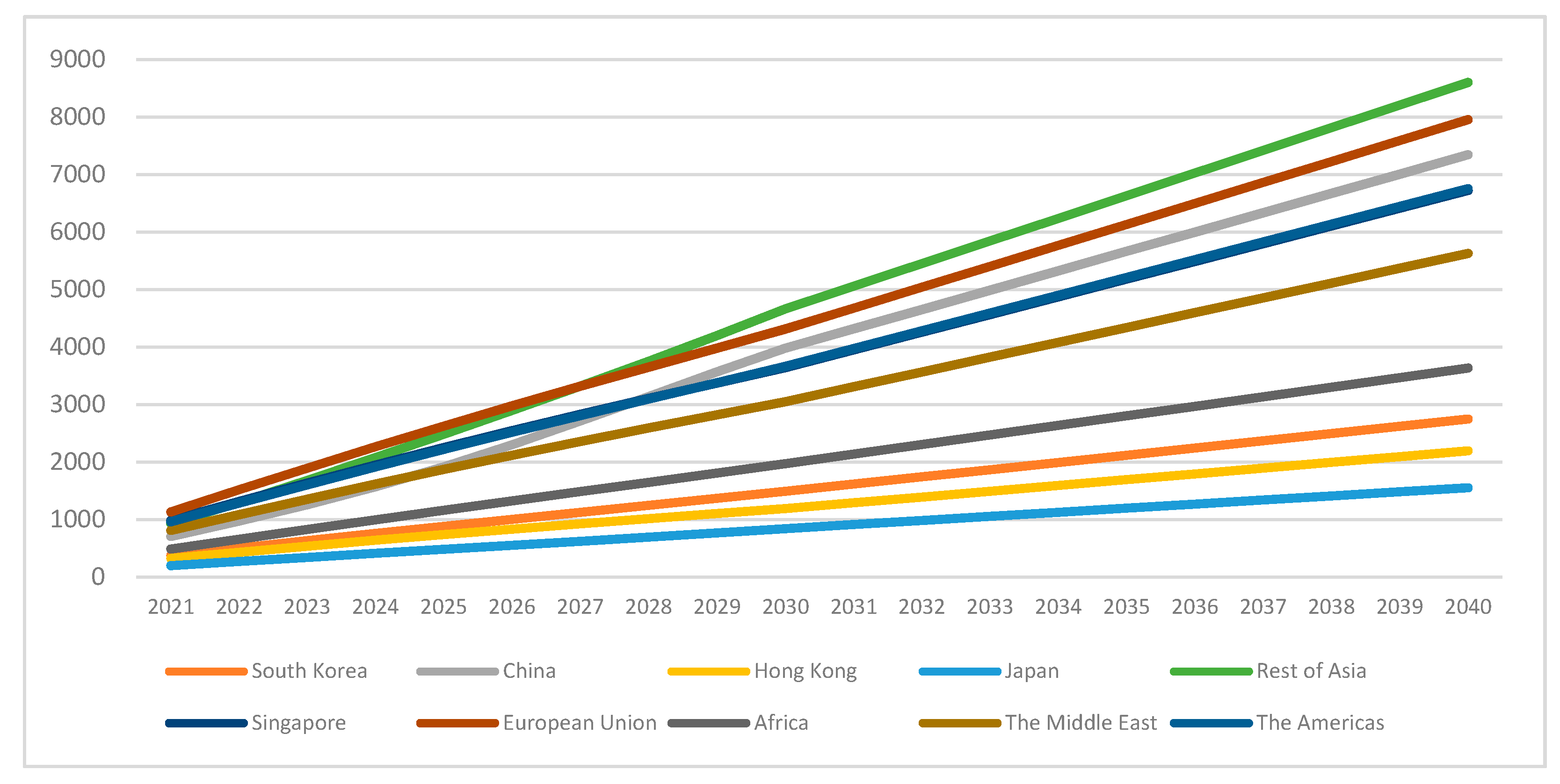
LNG bunkering demand by country and region was estimated using the results of the global LNG bunkering demand forecast and the LNG bunkering ratios by country and region. First, the results of Scenario 1 (the most likely) for the 2021–2040 period are as shown in Figure 4. Demand in the EU increased 604% from 1.1 to 8.0 million tons. Demand in Singapore grew 585% from 1.0 to 6.7 million tons. In the Americas, demand grew 604% from 1.0 to 6.8 million tons. In the rest of Asia, demand grew 827% from 0.9 to 8.6 million tons, exceeding the demand in the EU in 2027. In the Middle East, demand rose 595% from 0.8 million tons to 5.6 million tons. In China, demand showed an increase of 941% from 0.7 million tons to 7.3 million tons, surpassing the Middle East in 2025 and Singapore in 2028. Demand in South Korea increased 635% from 0.4 to 2.7 million tons. In Japan, demand rose 684% from 0.2 to 1.6 million tons.

Second, the results of Scenario 2 (the industry friendly scenario) for the 2021–2040 period are as shown in Figure 5. In the EU, demand increased 644% from 1.3 to 10.0 million tons. In Singapore, demand rose 624% from 1.2 to 8.5 million tons. Demand in the Americas grew 645% from 1.1 to 8.5 million tons. In the rest of Asia, demand grew 880% from 1.1 to 10.8 million tons, exceeding demand in the EU in 2027. In the Middle East, demand rose 635% from 1.0 million tons to 7.1 million tons. In China, demand increased 1002% from 0.8 to 9.2 million tons, surpassing the Middle East in 2025 and Singapore in 2028. In South Korea, demand increased 678% from 0.4 to 3.5 million tons. Demand in Japan rose 730% from 0.2 to 2.0 million tons.

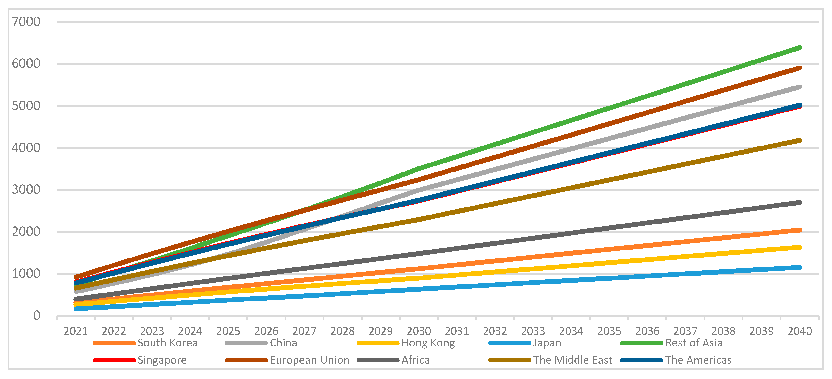
Last, the results of Scenario 3 (the environmentally friendly scenario) for the 2021–2040 period are as follows (see Figure 6). In the EU, LNG bunkering demand increased 544% from 0.9 to 5.9 million tons. Singapore experienced a 527% increase from 0.8 to 5.0 million tons. The Americas experienced a 544% increase from 0.8 to 5.0 million tons. In the rest of Asia, demand grew 748% from 0.8 to 6.4 million tons. In 2027, the LNG bunkering demand in the rest of Asia was found to exceed of the EU. The Middle East’s demand rose 536% from 0.7 to 4.2 million tons. China’s demand grew 853% from 0.6 to 5.4 million tons, surpassing that of the Middle East in 2025 and Singapore in 2028. Demand in South Korea experienced a 573% increase from 0.3 to 2.0 million tons; that in Japan showed an increase of 618% from 0.2 to 1.2 million tons.

4.4. Comparison with Previous Findings

The results of this study were compared with the relevant literature. As depicted in

Table 7. Global LNG bunkering demand forecast, comparison with previous studies (unit: 1000 tons).

	2025	2030	2035	2040
Scenario 1	16,635	28,810	40,984	53,159
IHS (2017)	16,500	27,600	43,900	70,000
IHS (2020)	19,300	31,200	45,700	65,700
IEA New Policy (2017)	23,900	29,700	36,200	41,300
IEA New Policy (2019)	7800	15,800	25,100	37,000
MOF (2018)	12,925	14,712	24,462	24,269

, IHS Markit and the IEA recently released two forecasting results. Both organizations’ forecasts are increasing in demand for LNG bunkering from 2025 to 2040. The forecasting demand of IHS (2017) increased from 16,500 thousand tons to 70,000 thousand tons, and expected result of IHS (2020) showed a growth from 19,300 thousand tons to 65,700 thousand tons. LNG bunkering demand of IEA (2017) rose from 23,900 thousand tons to 41,300 thousand tons, and prediction result of IEA (2019) grew from 7800 thousand tons to 37,000 thousand tons. Table 7 shows the Global LNG bunkering demand forecast, comparison with previous studies.

However, the latest forecast is lower than the previous one. The reason seems to be due to each country’s official reduction pledges to Paris Climate Change Accord, expansion of energy transition policies, and the development of energy technology [60].

First, we compared our results with the IHS forecast. Our estimates for 2025 and 2030 were consistent with those of the IHS (2017), but the present result for 2035 and 2040 was lower than the IHS’s prediction (2017, 2020).

Second, we compared our results from scenario 1 (most likely) with those of the IEA (2017). While the numbers for 2025 and 2030 predicted lower demand than the IEA (2017), our forecasts for 2035 and 2040 were higher than those of the IEA (2017). We showed higher demand than the IEA (2019) forecast. This study also presented higher demand than the MOF in South Korea’s forecast. Overall, the present estimates fall in the middle of those of existing studies.

As mentioned in the literature review, the predicted results appear differently according to the assumptions, methodology, data, and human skills in question. Predictions assume that past causal relationships will continue in the future. In general, prediction has intrinsic properties not only the actual result and the predicted value are different but also prediction accuracy decreases as the time passes. Therefore, repeatedly performing predictions are essential for reducing errors. It is for this reason that international organizations perform forecasts several times.

5. Discussion

In 2020, the IMO strengthened regulations pertaining to ship emissions to protect public health and the environment. Governments are also strengthening their policies to cope with climate change. Currently, there is great emphasis on sustainability among all stakeholders. Therefore, social awareness to LNG-powered ships and LNG bunkering is increasing. Compared to other alternatives, LNG fuel can help avoid air pollution such as that caused by sulfur oxide, nitrogen oxides, and fine dust. Additionally, it has the benefits of carbon reduction and low costs. Despite these benefits, the international community no longer considers it a solution to address climate change [61,62]. Nevertheless, LNG bunkering has become the industry’s most realistic alternative. The aim of the present study was to predict LNG bunkering demand globally and by individual country and/or region.

This paper predicted LNG bunkering demand using a top-down approach. First, global LNG bunkering demand was estimated through meta-regression analysis. Second, LNG bunkering demand by country and region was estimated. The analogy method, which reflected the oil bunkering ratio of each country as the LNG bunkering ratio, was applied. The oil bunkering demand forecast by country and region used existing data to predict demand from 2015 to 2040.

This study has identified that demand for LNG bunkering is expected to grow rapidly. This finding broadly supports other studies in the LNG bunkering forecast field [6,8,27]. Regarding global LNG bunkering demand, the results predicted an increase from 6.9 million tons in 2021 to 53.2 million tons by 2040. The results of each country/region’s forecasts were interesting. One unanticipated finding was that the LNG bunkering demand in the rest of Asia countries will overtake that of the EU in 2027. This is a significant finding when considering the fact that, at present, the EU is the hotspot of LNG bunkering infrastructure [6]. It seems possible that this result is due to the steady economic growth of Southeast Asian countries. The governments and industry, which want to secure industrial leadership, need to consider the growth of Southeast Asian countries. The development of Southeast Asian economies and their effect on the LNG bunkering industry may be a fruitful area for further research. China’s LNG bunkering growth, even without Hong Kong, will overtake Singapore in 2028. In the Asian region, markets will be formed in the order of China, Singapore, South Korea and Japan. Liquified natural gas bunkering demand in Asia will surpass the demand outside of Asia; however, the EU will remain a traditional power in the future. Market growth in the Middle East and Africa will be steady.

The forecast for LNG bunkering demand is largely influenced by policy implementations and economic conditions [14]. Demand for LNG fuel depends on the intensity of policy implementations by the IMO and governments in response to climate change. The economic conditions include the LNG ships chosen by shipping companies, the adoption of LNG bunkering infrastructure, oil prices, the size of new ships, and the changes in the employment of the ships [5,6,12,63]. LNG Demand forecasting results of the IEA (2019) was lower than those of the IEA (2017). Although there was no clear explanation of the prediction gap, the IEA (2019) mentioned some reasons for the uncertainty of LNG vessel growth and the fact that methane slip makes little difference between LNG and marine diesel with regards to greenhouse gas benefits. Therefore, it is evident that LNG demand forecasting is sensitive to various conditions. Overall, if many conglomerates choose LNG-powered ships, LNG will play a major role as a ship fuel over the next 20 years [14].

Two limitations of this study deserve mentioning. First, as the LNG bunkering market is in an early stage, there are no historical data for analysis. To counter this problem, we used the analogy method, however it is difficult to say that demand for oil bunkering and LNG bunkering behave in the same way. Second, it is important to consider other variables. International organizations’ and governments’ willingness to enforce environmental policies will be a major variable. At the same time, the willingness of business groups to follow these policies is also important. In addition, the results of this study may change depending on LNG supply, demand, and price.

Despite these limitations, this study can be used as an important data for the implementation of environmental policies by international organizations and governments. It also suggests strategic moves for the LNG bunkering industry. Demand forecasting is essential for investment to vitalize the LNG bunkering industry. For example, predictions are vital for governments to properly establish LNG bunkering port networks to facilitate the smooth operation of LNG-powered ships. In addition, this study establishes a quantitative framework for LNG bunkering demand predictions, which has not been presented in previous research. The results of this study will reduce the inherent uncertainty of the future LNG bunkering market and improve its forecasting power.

References

1. Viana, M.; Hammingh, P.; Colette, A.; Querol, X.; Degraeuwe, B.; de Vlieger, I.; van Aardenne, J. Impact of maritime transport emissions on coastal air quality in Europe. Atmos. Environ. 2014, 90, 96–105. [Google Scholar] [CrossRef]
2. Eyring, V.; Isaksen, I.S.A.; Berntsen, T.; Collins, W.J.; Corbett, J.J.; Endresen, O.; Grainger, R.G.; Moldanova, J.; Schlager, H.; Stevenson, D.S. Transport impacts on atmosphere and climate: Shipping. Atmos. Environ. 2010, 44, 4735–4771. [Google Scholar] [CrossRef]
3. Corbett, J.J.; Winebrake, J.J.; Green, E.H.; Kasibhatla, P.; Eyring, V.; Lauer, A. Mortality from ship emissions: A global assessment. Environ. Sci. Technol. 2007, 41, 8512–8518. [Google Scholar] [CrossRef]
4. Anderson, M.; Salo, K.; Hallquist, A.M.; Fridell, E. Characterization of particles from a marine engine operating at low loads. Atmos. Environ. 2015, 101, 65–71. [Google Scholar] [CrossRef] [Green Version]
5. Korea Maritime Institute (KMI). Port Strategies Following the Introduction of LNG-Fuelled Ships; Korea Maritime Institute: Busan, Korea, 2015; Available online: https://www.kmi.re.kr/web/board/view.do?rbsIdx=113&key=LNG+%EC%B6%94%EC%A7%84%EC%84%A0+%EB%8F%84%EC%9E%85&keyField=search1&idx=37022 (accessed on 25 May 2021).
6. Peng, Y.; Zhao, X.Z.; Zuo, T.L.; Wang, W.Y.; Song, X.Q. A systematic literature review on port LNG bunkering station. Transp. Res. D Transp. Environ. 2021, 91. [Google Scholar] [CrossRef]
7. Van, T.C.; Ramirez, J.; Rainey, T.; Ristovski, Z.; Brown, R.J. Global impacts of recent IMO regulations on marine fuel oil refining processes and ship emissions. Transp. Res. D Transp. Environ. 2019, 70, 123–134. [Google Scholar] [CrossRef]
8. Park, N.K.; Park, S.K. A Study on the Estimation of Facilities in LNG Bunkering Terminal by Simulation-Busan Port Case. J. Mar. Sci. Eng. 2019, 7, 354. [Google Scholar] [CrossRef] [Green Version]
9. DNV-GL. Maritime Forecast to 2050: Energy Transition Outlook 2019; DNV-GL: Hamburg, Germany, 2019. [Google Scholar]
10. Total. Developing a global LNG bunkering infrastructure. In Proceedings of the International LNG Fueled Ship & Bunkering Conference, Busan, Korea, 10 December 2019. [Google Scholar]
11. Iannaccone, T.; Landucci, G.; Tugnoli, A.; Salzano, E. Sustainability of cruise ship fuel systems: Comparison among LNG and diesel technologies. J. Clean. Prod. 2020, 260. [Google Scholar] [CrossRef]
12. The Ministry of Oceans and Fisheries (MOF). A Study on the Construction of LNG Bunkering Infrastructure of Major Ports in Korea-Final Report; Ministry of Oceans and Fisheries: Sejong, Korea, 2018. [Google Scholar]
13. DNV-GL. Global status and outlook of LNG fuelled ship and LNG bunkering. In Proceedings of the International LNG Fuelled Ship and Bunkering Conference 2019, Busan, Korea, 10 December 2019; pp. 25–37. [Google Scholar]
14. The Oxford Institute for Energy Studies. A Review of Demand Prospects for LNG as a Marine Transport Fuel; University of Oxford: Oxford, UK, 2018. [Google Scholar] [CrossRef]
15. IHS Markit. IHS Markit LNG Long-Term Scenarios to 2050; LNG in Transportation Outlooks at Excel Sheet Data; IHS Markit: London, UK, 2020. [Google Scholar]
16. International Energy Agency (IEA). World Energy Outlook 2019; International Energy Agency: Paris, France, 2019. [Google Scholar]
17. S&P Global Platts. How the IMO 2020 regulation will impact the LNG market. In Proceedings of the 19th International Conference & Exhibition on Liquefied Natural Gas, Shanghai, China, 2–5 April 2019. [Google Scholar]
18. Gazprom. LNG as future transport in Europe. In Proceedings of the 4th Annual Baltic Energy Summit, Tallinn, Estonia, 13–15 November 2012. [Google Scholar]
19. Society for Gas as a Marine Fuel. International LNG fueled ship & bunkering. In Proceedings of the International LNG Fueled Ship & Bunkering Conference, Busan, Korea, 10 December 2019. [Google Scholar]
20. De Villota, E.D.; Carmona, M.T.G.; Rubio, J.J.; de Andrés, S.R. Equality of the in vivo and in vitro oxygen-binding capacity of haemoglobin in patients with severe respiratory disease. Br. J. Anaesth. 1981, 53, 1325–1328. [Google Scholar] [CrossRef] [Green Version]
21. Tamura, I.; Tanaka, T.; Kagajo, T.; Kuwabara, S.; Yoshioka, T.; Nagata, T.; Kurahashi, K.; Ishitani, H. Life cycle CO2 analysis of LNG and city gas. Appl. Energy 2001, 68, 301–319. [Google Scholar] [CrossRef]
22. Smith, A.B. Gas fuelled ships: Fundamentals, benefits classification & operational issues. In Proceedings of the First Gas Fuelled Ships Conference, Hamburg, Germany, 26–27 November 2010. [Google Scholar]
23. Bekaert, M. LNG as Fuel for Shipping; Gassforum: Brussels, Belgium, 2016. [Google Scholar]
24. Pfoser, S.; Schauer, O.; Costa, Y. Acceptance of LNG as an alternative fuel: Determinants and policy implications. Energy Policy 2018, 120, 259–267. [Google Scholar] [CrossRef]
25. Burel, F.; Taccani, R.; Zuliani, N. Improving sustainability of maritime transport through utilization of Liquefied Natural Gas (LNG) for propulsion. Energy 2013, 57, 412–420. [Google Scholar] [CrossRef]
26. Kumar, S.; Kwon, H.T.; Choi, K.H.; Lim, W.; Cho, J.H.; Tak, K.; Moon, I. LNG: An eco-friendly cryogenic fuel for sustainable development. Appl. Energy 2011, 88, 4264–4273. [Google Scholar] [CrossRef]
27. Wan, C.P.; Yan, X.P.; Zhang, D.; Yang, Z.L. A novel policy making aid model for the development of LNG fuelled ships. Transp. Res. A Policy Pract. 2019, 119, 29–44. [Google Scholar] [CrossRef]
28. Aronietis, R.; Sys, C.; Hassel, E.V.; Vanelslander, T. Forecasting port-level demand for LNG as a ship fuel: The case of the port of Antwerp. J. Shipp. Trade 2016, 1, 1–22. [Google Scholar] [CrossRef] [Green Version]
29. Bengston, S.; Andersson, K.; Fridell, E. A comparative life cycle assessment of marine fuels: Liquefied natural gas and three other fossil fuels: Proceedings of the institution of mechanical engineers, Part M. J. Eng. Mar. Environ. 2011, 225, 97–110. [Google Scholar]
30. Najm, S.; Matsumoto, K. Does renewable energy substitute LNG international trade in the energy transition? Energy Econ. 2020, 92, 104964. [Google Scholar] [CrossRef]
31. Ahad, A.-E.; Eric, C.O.; Yusuf, B.; Tareq, A.-A. A review of cleaner alternative fuels for maritime transportation. Energy Rep. 2021, 7, 1962–1985. [Google Scholar] [CrossRef]
32. Weng, Y. The development of marine LNG infrastructure starts a good time. China Ship Surv. 2019, 2, 44–46. [Google Scholar]
33. Kim, H.S.; Choi, K.H. A Study on the Development and Operation of LNG Bunkering Hub Port in Korea. Korea Int. Commer. Rev. 2018, 33, 335–352. [Google Scholar]
34. Lee, J.S. Legal Issues on LNG Bunkering to Respond to IMO Regulations to Reduce Sulfur Oxide Emission from Ships. Environ. Law Rev. 2019, 41, 163–200. [Google Scholar] [CrossRef]
35. Wang, H. Research on LNG Refueling Station Site Selection Direction; Dalian Maritime University: Dalian, China, 2014. [Google Scholar]
36. Wang, L. Research on the Development Forecast of Chongqing Marine LNG Bunkering Terminal Layout Planning. China Water Transp. 2014, 14, 279–280, 317. [Google Scholar]
37. Yang, Y. Planning Site Selection and Evaluation for Coastal Port LNG Fuel Power Ship Filling Station; Harbin Institute of Technology: Harbin, China, 2016. [Google Scholar]
38. Liu, Z. Research on Market Forecast of waterborne LNG Bunkering Station. Gas Heat 2020, 40, 24–28, 45–46. [Google Scholar] [CrossRef]
39. Lee, C.-Y.; Huh, S.-Y. Forecasting new and renewable energy supply through a bottom-up approach: The case of South Korea. Renew. Sustain. Energy Rev. 2017, 69, 207–217. [Google Scholar] [CrossRef]
40. Kahn, K.B. New Product Forecasting: An Applied Approach; Routledge: New York, NY, USA, 2006. [Google Scholar]
41. Jacobsen, H.K. Integrating the bottom-up and top-down approach to energy economy modelling: The case of Denmark. Energy Econ. 1998, 20, 443–461. [Google Scholar] [CrossRef] [Green Version]
42. Frei, C.W.; Haldi, P.A.; Sarlos, G. Dynamic formulation of a top-down and bottom-up merging energy policy model. Energy Policy 2003, 31, 1017–1031. [Google Scholar] [CrossRef]
43. McFarland, J.R.; Reilly, J.M.; Herzog, H.J. Representing energy technologies in top-down economic models using bottom-up information. Energy Econ. 2004, 26, 685–707. [Google Scholar] [CrossRef] [Green Version]
44. Rivers, N.; Jaccard, M. Combining top-down and bottom-up approaches to energy-economy modeling using discrete choice methods. Energy J. 2005, 26, 83–106. [Google Scholar] [CrossRef] [Green Version]
45. Dai, H.; Mischke, P.; Xie, X.; Xie, Y.; Masui, T. Closing the gap? Top-down versus bottom-up projections of China’s regional energy use and CO2 emissions. Appl. Energy 2016, 162, 1355–1373. [Google Scholar] [CrossRef]
46. Yuan, Y.; Wang, M.; Zhu, Y.; Huang, X.; Xiong, X. Urbanization’s effects on the urban-rural income gap in China: A meta-regression analysis. Land Use Policy 2020, 99, 104995. [Google Scholar] [CrossRef]
47. Nagy, B.; Farmer, J.D.; Bui, Q.M.; Trancik, J.E. Statistical Basis for Predicting Technological Progress. PLoS ONE 2013, 8. [Google Scholar] [CrossRef] [Green Version]
48. Korea Institute for International Economic Policy. Trade Liberalization and Productivity Growth: An Analysis on the Mechanism for Productivity Growth; Korea Institute for International Economic Policy: Sejong, Korea, 2008. [Google Scholar]
49. Nelder, J.A.; Wedderburn, R.W.M. Generalized linear models. J. R. Stat. Soc. 1972, 135, 370–384. [Google Scholar] [CrossRef]
50. Dong, S.; Wang, P.; Abbas, K. A survey on deep learning and its applications. Comput. Sci. Rev. 2021, 40. [Google Scholar] [CrossRef]
51. Naga, D.S.K.; Venkatramaphanikumar, S.; Venkata, K.K.K.; Debnath, B. Review on the Usage of Deep Learning Models in Multi-modal Sentiment Analysis. IEIE Trans. Smart Process. Comput. 2020, 9, 435–444. [Google Scholar] [CrossRef]
52. Breiman, L. Random forests. Mach. Learn. 2001, 45, 5–32. [Google Scholar] [CrossRef] [Green Version]
53. Chen, Y.Y.; Zheng, W.Z.; Li, W.B.; Huang, Y.M. Large group activity security risk assessment and risk early warning based on random forest algorithm. Pattern Recognit. Lett. 2021, 144, 1–5. [Google Scholar] [CrossRef]
54. Makungwe, M.; Chabala, L.M.; Chishala, B.H.; Lark, R.M. Performance of linear mixed models and random forests for spatial prediction of soil pH. Geoderma 2021, 397, 115079. [Google Scholar] [CrossRef]
55. Deng, S.K.; Wang, C.G.; Wang, M.Y.; Sun, Z. A gradient boosting decision tree approach for insider trading identification: An empirical model evaluation of China stock market. Appl. Soft Comput. 2019, 83. [Google Scholar] [CrossRef]
56. Liu, J.-J.; Liu, J.-C. An intelligent approach for reservoir quality evaluation in tight sandstone reservoir using gradient boosting decision tree algorithm—A case study of the Yanchang Formation, mid-eastern Ordos Basin, China. Mar. Pet. Geol. 2021, 126, 104939. [Google Scholar] [CrossRef]
57. Lee, S. Monte Carlo simulation using support vector machine and kernel density for failure probability estimation. Reliab. Eng. Syst. Saf. 2021, 209, 107481. [Google Scholar] [CrossRef]
58. International Energy Agency (IEA). World Energy Outlook 2016; International Energy Agency: Paris, France, 2016. [Google Scholar]
59. Wang, S.; Wang, J.; Lu, H.; Zhao, W. A novel combined model for wind speed prediction—Combination of linear model, shallow neural networks, and deep learning approaches. Energy 2021, 234, 121275. [Google Scholar] [CrossRef]
60. Korea Energy Economics Institute (KEEI). A Study on the Bunkering Industry Response Strategies for Strengthening Environmental Regulations of the International Maritime Organization; KEEI: Ulsan, Korea, 2020; Available online: https://www.keei.re.kr/main.nsf/index.html (accessed on 25 May 2021).
61. Kah, M. The future of hydrocarbons: Changing demand and subsequent impacts “projections for oil and natural gas demand”. In Proceedings of the 1st IAEE Middle East Symposium, Association for Energy Economics, Abu Dhabi, United Arab Emirates, 16–18 December 2019. [Google Scholar]
62. Kah, M. Columbia Global Energy Dialogue: Natural Gas Flaring Workshop Summary. 2020. Available online: https://energypolicy.columbia.edu/research/global-energy-dialogue/columbiaglobal-energy-dialogue-natural-gas-flaring-workshop-summary (accessed on 25 May 2021).
63. Schinas, O.; Butler, M. Feasibility and commercial considerations of LNG-fueled ships. Ocean Eng. 2016, 122, 84–96. [Google Scholar] [CrossRef]
Figure 1. Research flow.
Sustainability 13 09058 g001
Figure 2. Global LNG bunkering demand forecast.
Sustainability 13 09058 g002
Figure 3. Deep learning prediction results for oil bunkering by country/region (unit: 1000 ton).
Sustainability 13 09058 g003
Figure 4. Global liquified natural gas bunkering demand forecast by country/region based on Scenario 1 (unit: 1000 tons).
Sustainability 13 09058 g004
Figure 5. Global liquified natural gas bunkering demand forecast by country/region based on Scenario 2 (unit: 1000 tons).
Sustainability 13 09058 g005
Figure 6. Global liquified natural gas bunkering demand forecast by country/region based on Scenario 3 (unit: 1000 tons).
Sustainability 13 09058 g006