Optimized Expansion Strategy for a Hydrogen Pipe Network in the Port of Rotterdam with Compound Real Options Analysis

Abstract

The port of Rotterdam is the largest seaport in Europe. To maintain its position, the harbor will have to anticipate global transitions such as transferring to sustainable energy. Hydrogen is seen as a promising energy carrier; however, future demand is uncertain. The current research investigates decision making under uncertainty and values flexibility. Compound real options analysis is applied to optimize the time-variant expansion strategies for a hydrogen pipe network. The trade-off between early investments and missed revenues when not investing in time determines the optimized expansion strategy. Moreover, the real options approach also provides the levelized unit price for hydrogen distribution, to cover the life cycle costs of the optimal expansion strategy. Finally, this real options approach offers flexibility to a decision maker as it allows for enhancing future decisions. The academic contribution of this research is a distinct perspective on a compound real options approach where the optimal strategic path is the key result of interest. This in contrast to other real options applications in the literature which focus on option value, exchange with limiting the options or do not visualize a strategic path. Moreover, this research demonstrates how stepwise expansion and decision making under uncertainty facilitate transitions such as the transition toward clean energy.

1. Introduction

Global warming imposes severe threats to ecosystems and especially to densely populated urban deltas which are prone to flooding [1,2,3]. The Intergovernmental Panel on Climate Change (IPCC) warns of unprecedented consequences of global warming beyond 1.5 °C. Global warming is currently developing at a faster pace than originally anticipated on [3,4]. The IPCC stresses the importance of keeping global warming below its critical threshold, but this requires huge and radical transformations to reduce greenhouse gasses that emerge from burning fossil fuels. At the same time, the IPCC foresees a growing demand for energy.

Ports and especially seaports play an important role in this growing demand for clean energy as being energy generators, consumers and transporters [5,6]. Ports consume energy for their logistics operations. Moreover, port industry and shipping consume large amounts of energy. Ports also generate energy and benefit from their locations and natural resources such as wind and waves. Additionally, ports play an important role in the throughput of energy. The generated power is not only for port activities but also for distribution to the hinterland. Ports are energy hubs and are precursors in the transition toward clean energy [5,6]. Developments in clean energy are seen in ports all over the world and are geared at biofuels such as LNG, solar panels, wind farms, hydrogen, geothermal energy, power to gas concepts and carbon capture and storage. These developments also stress the growing need for integrated energy management planning [6]. Two case studies (Hamburg and Genoa) presented by [5] demonstrate the importance of strategic planning for energy management in ports because ports are strongly tied to their environment.

Moreover, integrated clean energy concepts also induce a growing need for energy management systems to optimize supply from different integrated energy sources. This is illustrated in [7], whose authors developed a one-day-dispatch supply model for an integrated power-heat system. In addition, [6] demonstrates how the energy supply of an integrated clean energy concept can be optimized by using a multi-objective optimization approach. However, it is not just the operational strategy of energy supply that needs to be optimized in ports. Investments need to be optimized as well. Previous work optimizes the management of smart port grids after these energy systems are built, whereas the current research focuses on the phased introduction of a clean energy system in the port of Rotterdam under an uncertain demand for the source of energy. The port of Rotterdam is the largest seaport in Europe, with nearly 30,000 sea-going vessels arriving in 2020 and a freight throughput of nearly 440 million tons. To maintain its position, the harbor anticipates global transitions such as transferring to sustainable energy in accordance with the United Nations’ sustainable development goals. Hydrogen is seen as the promising alternative sustainable energy carrier to contribute to these goals [8].

The port of Rotterdam aims to become an international hub for the production, import and throughput of hydrogen. Hydrogen will gradually replace natural gas. By 2050 the port of Rotterdam anticipates receiving annually, on average, 18 million tons of green hydrogen. This hydrogen is meant as a feedstock for the port industry (refineries), fuel for shipping and heavy land transport, and power for port activities. This green hydrogen is also meant for export to Northwestern Europe and will be used for district heating and provision of heating to greenhouses in the Western part of the Netherlands [8]. An important aspect of realizing these ambitions is the construction of a backbone pipeline for large scale transportation of hydrogen [8]. Transition to hydrogen as an alternative energy carrier contributes to the Dutch National Climate goals of a 50% reduction of CO₂ emissions in 2030, and a full reduction in 2050 compared to 1990 [9].

These radical transformations toward sustainable energy are, by definition, very costly, and at the same time, they are subject to uncertainties about demand, price developments and future technologies. Valuing these investments with traditional (NPV) comparison hampers the phased introduction of new technology because traditional NPV comparison cannot value the flexibility of a decision maker. A decision maker can enhance future decisions when more information becomes available [10,11,12,13,14]. Traditional NPV comparison does not facilitate adaptive design or multi-staged expansions [14,15,16]. In contrast Real Options Analysis (ROA) is an approach which facilitates decision making under uncertainty and values the flexibility to enhance future decisions in response to how uncertainty evolves [17,18,19,20,21]. The application of ROA allows decision-makers to optimize and enhance a sequence of such decisions [22,23,24]. It is therefore not surprising that ROA is embraced in the energy sector to support the transition toward sustainable energy [14,15,16,25,26,27,28]. Despite the many advantages and the ROA applications available in the scientific literature, there are still a number of challenges identified in the application of ROA. Wang and Neufville [29] observe that many ROA applications do not consider interdependencies between options, an observation recently confirmed by [16,24] and the current research. Most ROA applications in the literature are single-timing options (delay or invest) instead of path-dependent compound options (for example, a sequence of expansions).

Moreover, it is observed by [30] that the acceptance of ROA outcomes by a decision maker is tied to the understanding of how the model values flexibility. Many ROA applications are built on Monte Carlo simulations. This method facilitates the inclusion of multiple uncertainty variables but will also result in outcomes to be perceived as a black box. In addition, the choice for the stochastic processes to be simulated and their underlying descriptive parameters are subject to debate. As an example, a Geometric Brownian Motion (GBM) is popular for predicting stock price developments, however, many authors argue whether this assumption holds for the prediction of prices in real projects [19,29,31,32]. Similar findings are presented by [24], whose authors challenge the practical relevance of many ROA applications given the absence of compound options, the assumptions on uncertainty quantification, the mathematical complexity and the lack of empirical evidence in real-life cases.

The current research investigates the optimal phased expansion of a hydrogen pipeline network in a real-life case study where the aforementioned challenges are addressed. This case study is in the port of Rotterdam, however, the ROA approach developed in this study is methodologically transferable to other challenges with compound options. Not so much the option value, but the identification of the optimal strategic path, is the key result of interest, in contrast to the literature reviewed and discussed in Section 4. Moreover, the compound ROA application is used to calculate the levelized unit price for hydrogen to cover the life cycle costs of the optimal path.

The outline of this paper is as follows. Section 2 presents the ROA modelling approach for the case study. Section 3 presents the results of the case study, including a sensitivity analysis and the limitations of the model. Section 4 discusses the application of ROA from both a methodological perspective and a more generalized perspective for decision making. This paper is finalized with conclusions in Section 5.

2. Materials and Methods

The case study is conducted in the context of the energy transition in the port of Rotterdam. In line with the Dutch National Climate targets, the port authority aims to decarbonize activities in the port area and the maritime sector [33,34]. The technical feasibility of hydrogen as an alternative energy carrier in the port of Rotterdam is elaborated on in the H-vision document of the port authority and affiliated organizations [9]. This document presents future scenarios which build on existing technology and, where possible, the reuse of existing industrial infrastructure. Until 2030, blue hydrogen is anticipated on and seen as the enabler toward the large-scale provision of green hydrogen hereafter. The later will be possible in the Netherlands as soon as wind and solar energy will be amply available at competitive prices. Chemically, all types of hydrogen are the same, however, the production of hydrogen differs. Roughly, there are three forms of hydrogen, so-called grey, blue and green hydrogen. Grey hydrogen is produced with the use of fossil fuels. Blue hydrogen is also produced with the use of fossil fuels or nuclear power, however, in contrast with grey hydrogen, CO₂ emissions are captured and stored; here, in empty North-Sea gas fields. Green hydrogen is produced using renewable energy and has zero to negligible CO₂ emissions. Blue hydrogen can quickly be made available. It accelerates the large-scale introduction of green hydrogen as it also implements the required infrastructure.

The scenarios combine the expected future hydrogen demand of the industry sector in the port of Rotterdam as well as the demand that is ought to be transported through the port and distributed to the hinterland. Four representative scenarios are subtracted from [9] to be used in the ROA. These scenarios cover a maximum range of potential developments. Moreover, these scenarios are extended to include the demand for hydrogen that is transported through the port based on the expectations of the port authority.

The decarbonization goals are ambitious, the practical translation and implications are as of yet uncertain and abstract. In this case study, the aim is to translate the strategic hydrogen ambitions to a preliminary long-term adaptive strategy for a new hydrogen pipeline network in the port of Rotterdam by applying ROA. Moreover, this study aims to give an indication of the case-specific levelized unit price for hydrogen to cover the life cycle costs of the optimal strategy. The ROA strategy optimizes a time-variant sequence of expansion decisions for a hydrogen network under an uncertain demand development for hydrogen. Additionally, when this demand uncertainty decreases in the future as more information becomes available, the ROA approach allows for adjustment of the expansion strategies. These two ingredients, the optimization of a sequence of time-variant decisions and the possibility for future adjustments in optimizing this sequence of time-variant decisions, makes this approach an adaptive strategy.

To create a long-term adaptive expansion strategy the following steps are taken. First, scenarios for hydrogen transition in the port of Rotterdam are subtracted from the H-vision report [9]. Probabilities are assigned to the likelihood of occurrence of each scenario in the coming decennia. Second, flexible options are designed to meet this demand by the expansion of a pipeline network over time. These options are supported by pipeline diameter calculations and provide a foundation for the calculation of costs. Third, the options are combined in a decision tree to visualize the possible adaptive strategies. Hereafter the cost function is established to assign costs and revenues to each path in the decision tree, followed by a backward induction calculation to determine the optimal path in the decision tree. Finally, this case study is concluded with a sensitivity analysis. In the following sections, these methodological steps are elaborated on. The generalized method is summarized in Figure 1 and follows six steps, which are detailed in the following sections:

• Definition of scenarios for the development of demand and assessment of their realization probabilities over time. Existing recognized scenarios have been used and expanded with realization probabilities based on expert judgement. This is elaborated on in Section 2.1.
• Identification of the expansion options for meeting the various demands. Pipeline capacity calculations were deployed to find required nominal pipeline diameters. Hereafter, options for different configurations were identified based on available market sizes. This is detailed in Section 2.2.
• Development of a decision tree which visualizes the sequences of potential decisions over time. All sequential options (potential decisions) for capacity expansion have been modelled in a decision tree. Constructing a decision tree follows a generic process where decision nodes represent points in time where decisions can be taken, and arrows departing from these nodes represent the potential decisions. This is elaborated on in Section 2.3.
• Definition of the cost function and allocation of the costs and benefits to each possible future decision. Each decision comes with its costs and revenues. Costs for investments, operational expenditures and income missed when demand exceeds installed capacity. Each decision also comes with revenues for supplied demand. The cost function is defined in Section 2.4.
• Calculation of the optimal path in the decision tree by backward induction. Backward induction is an existing calculation technique and detailed in Section 2.5. Moreover, an illustrative generic optimal path calculation is provided in Appendix C.
• Assessment of the impact of other uncertainty variables with a sensitivity analysis. The presented method incorporates one uncertainty variable which is demand. This is a modelling choice because this study aims to visualize the optimal path in a compound real options approach. Inclusion of multiple uncertainties would turn the ROA into a black box. The other uncertainties such as costs and revenues are investigated with a sensitivity analysis afterwards. This provides insight in the magnitude of their impacts on the result (not a black box). The sensitivity analysis is provided in Section 3.2. A discussion from a methodological perspective with respect to the literature is provided in Section 4.1. This section also motivates modelling choices.

2.1. Scenarios for Development of Demand

Hydrogen is seen as an important energy carrier of the future. The ascent of a hydrogen economy is becoming a more realistic expectation [35]. The current research is focused on hydrogen transportation in the port of Rotterdam and subtracted the expected scenarios from H-vision [9]. These scenarios were developed by key stakeholders including the port of Rotterdam, the industry, utilities (gas, electricity) and the national and local governments. For the current research, additional interviews were conducted with seven experts on renewable energy and hydrogen development in the port of Rotterdam and/or the Netherlands. Their functions are: Program Manager: Pipelines, Spokesman: Business Operations, Project Engineer: Renewable Energy, Business Developer: New Energy, Senior Advisor: Strategy and Strategic Partnerships, Hydrogen Commercial Analysist and Energy Professional.

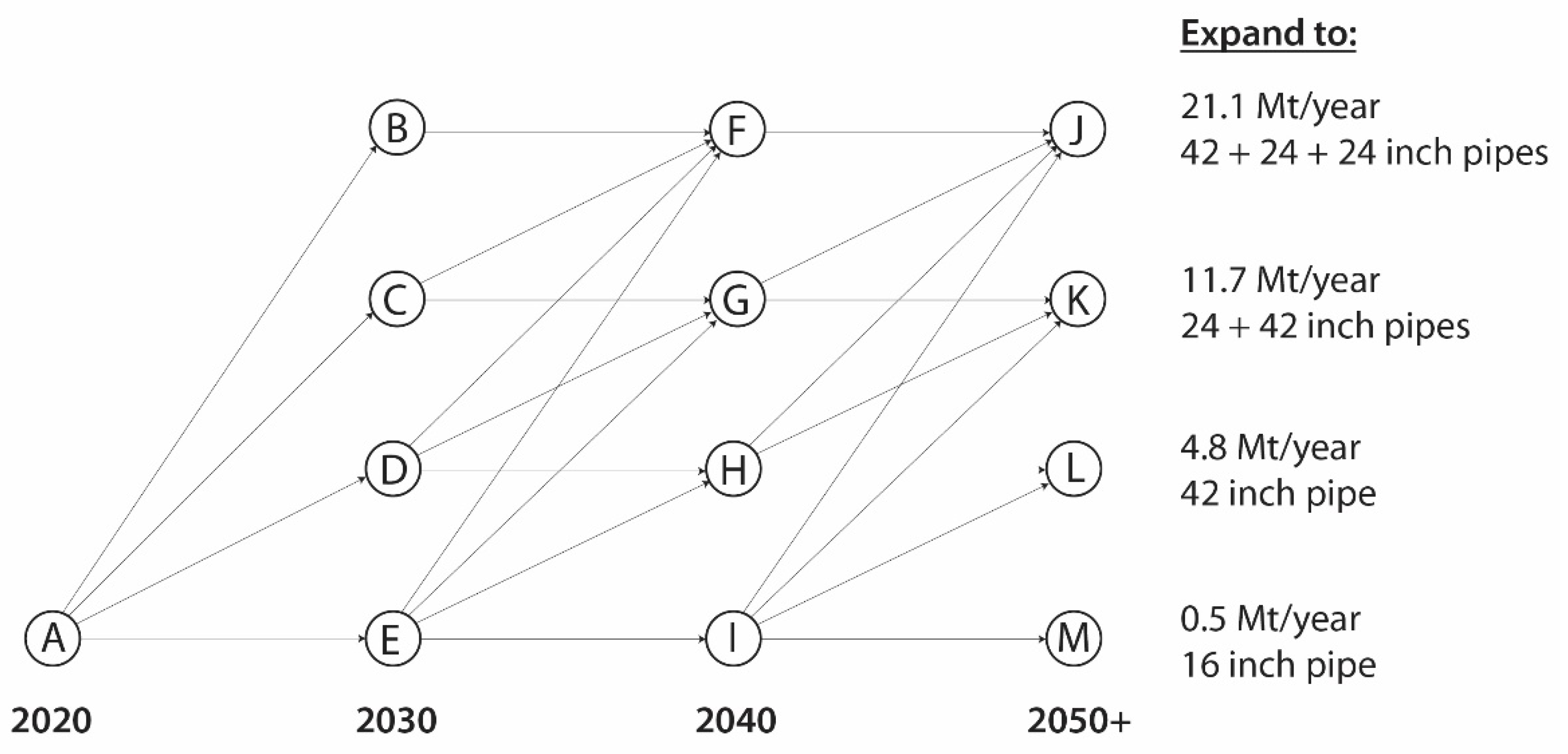
The scenarios build on existing technologies and reuse existing industrial infrastructure, and they are extended to include the demand for hydrogen that is transported through the port based on the expectations of the port authority. The expected total demand for hydrogen, expressed in million metric tons per year (Mt/y), for each scenario in 2050 is estimated at:

• Scenario A0 (baseline): a total demand of 0.5 Mt/y;
• Scenario A1 (minimal): a total demand of 4.8 Mt/y;
• Scenario B2 (medium): a total demand of 11.7 Mt/y;
• Scenario C3 (maximal): a total demand of 21.1 Mt/y.

Demand development over time is uncertain. Anticipating the timeline in the decision tree, the probabilities for the development of demand are established in consultation with the stakeholders of this research by expert judgment and shown in

Table 1. Probabilities for demand development per time interval.

Demand Development	2020–2030	2030–2040	2040–2050	>2050
Scenario A0: 0.5 Mt/y	40%	20%	5%	1%
Scenario A1: 4.8 Mt/y	45%	40%	35%	30%
Scenario B2: 11.7 Mt/y	10%	30%	35%	40%
Scenario C3: 21.1 Mt/y	5%	10%	25%	29%
Expected demand Mt/y	4.6	7.6	11.1	12.2

. The motivation is summarized as follows.

Period 2020–2030: At present, the port of Rotterdam is on the verge of a transition to hydrogen. The initiatives are driven by the Paris Agreement and Dutch National Climate Targets. However, the port of Rotterdam also depends on the demand for hydrogen by the port industry. In the first decade the stakeholders of this research do not expect a high probability for realization of the high demand scenarios for hydrogen as transitions take time (adaptation of infrastructure). The stakeholders expect going concern (baseline) and minimal growth to be the most likely scenarios in the first decade.

Period 2030–2040: In the second decade, the stakeholders of this research suspect a center of gravity around the minimal and medium demand scenarios for hydrogen demand because the climate targets enforce a realization of 50% of clean energy consumption, of which hydrogen is an important source. Industry is gradually making a transition to hydrogen.

Period 2040–2050: In the third decade, the demand for hydrogen is expected to increase. At the end of this decade, in 2050, the climate targets for 100% sustainable energy should be met. This very likely increases the medium and high demand scenarios. As hydrogen is not the only source of clean energy, the minimal growth scenario is also considered but with a lower probability.

Period after 2050: The climate targets should have been met. For the long term, the hydrogen demand is expected to gravitate around the medium growth scenario. The uncertainty is reflected in the likelihoods for the minimal growth scenario (as a consequence of alternative clean energy sources) and the maximal scenario (e.g., more export of hydrogen). This distribution of likelihoods reflects the notion that the future is more uncertain than the present.

These probabilities are used in balancing the costs of investments of expansion with the revenues which will be further detailed in Section 2.4. If installed capacity exceeds demand, too much was spent on expansion. If installed capacity is less than demand, potential income is lost.

2.2. Options for Supplying Demand

Hydrogen is supplied through pipelines, and various options are available for the phased expansion of pipelines. Nominal pipeline diameters for supplying the maximum demands per scenario are based on capacity calculations [9,36]. The nominal capacity calculations are translated into combinations of possible pipeline diameters capable of delivering the required demand. Pipeline diameters are available in fixed sizes within a range of 16 to 48 inch (400 mm to 1200 mm). Economically feasible options are presented in

Table 2. Possible options for pipeline diameters and compression capacities for supplying the required demands.

Annual Demand (Mt)	Compression Capacity (MW)	Nominal Diameter (Inch)	Options for Pipeline Diameters (Inch)
0.5	29.5	14	16
4.8	281	42	42
			36 + 16
11.7	692	66	24 + 42
			16 + 16 + 36
21.1	1242	89	42 + 48
			24 + 24 + 42
			16 + 36 + 42
			16 + 16 + 24 + 36

, and for this assessment, unit cost data were used [37].

In addition, compression capacities are required to transport hydrogen. These compression capacities are costly and cannot be ignored in an ROA. Compression capacities are estimated by using the North Sea Energy Technical assessment of hydrogen transport, compression, processing offshore [38]. The compression capacity is allocated to the total demand irrespective of the options for pipeline diameters. It is assumed that the same compression capacities and costs are required for similar options that combine pipeline diameters. The results following these calculations are also presented in Table 2.

2.3. Construction of a Decision Tree

Adaptive expansion strategies for supplying the hydrogen demands are visualized in a consolidated decision tree as depicted in Figure 2. The full decision tree with all the options for pipeline diameter configurations is presented in Appendix A, Figure A1. The tree consists of four stages for installed capacity. Each stage represents the supplied demand and contains the various options for the required pipeline diameters. The tree uses a time interval of 10 years, and each node offers the possibility to remain on the installed capacity or to expand to a higher capacity to meet higher demands.

The purpose of a decision tree is to first visualize all options (decisions) that are available to a decision maker. Each circle represents a decision node. Arrows depart from each decision node and represent the distinct decisions. As an example, in 2020, a decision maker has four options: Do nothing and move to node $E$ (remain at 0.5 Mt/y); expand to 4.8 Mt/y and move to node $D$; expand to 11.7 Mt/y and move to node $C$; or expand to 21.1 Mt/y and move to node $B$.

At present, it is not yet known what the best option for the decision maker is. This will be calculated after the full tree is constructed. Therefore, all options are taken into consideration as possibilities to choose from. For each node in 2030, again, all options are considered. If a decision maker would be in node $E$ in 2030, four options are available: move to $I$, $H$, $G$ or $F$.

However, if the decision maker would be in node $B$ in 2030, the maximum capacity has already been installed and only one option is available: remaining at the same capacity and moving to $F$ (assuming that once pipelines are constructed these are not decommissioned as the investments were spent). The remainder of the tree follows the same principle until the end nodes in 2050 are reached. From here onward, going concern is assumed as boundary constraints.

The decision tree visualizes all available options in each decision node. Each decision comes with distinct costs and revenues. These costs and revenues will be calculated and attributed to each arrow in the network, which is explained in Section 2.4. The probabilities for demand development, as depicted in Table 1, influence these costs and revenues. These probabilities are excluded from the visualization of the decision tree because probabilities are not decisions and will not alter the potentially available decisions. A decision maker would only experience the consequences after an irreversible decision is made in terms of costs and revenues and based on how demand develops. As such, the probabilities for demand development determine the costs and revenues to be attributed to the arrows in the decision tree.

After such a tree has been established, the shortest path through the network is calculated. The best successive choices for a decision maker follow this so-called shortest path in the entire network. In other words: when all possible decisions are known, and all costs and revenues are allocated to the arrows, the least cost route through the network can be calculated. The current research uses backward induction, which starts the calculation at the end nodes and systematically works back to the beginning of the tree (node $A$). This calculation is explained in Section 2.5.

2.4. Allocating Costs and Revenues to Each Path

Each decision, or transfer from one node to another, comes with costs and revenues. These are composed of the immediate investment ($I$) belonging to a decision, the successive annual operation and maintenance costs ($M$), the annual revenues for the hydrogen supply ($R$) and a potential penalty ($P$) if demand exceeds the capacity installed because of missed revenues. Each path has a duration of 10 years. All costs and revenues during these 10 years are discounted to the beginning of each path, resulting in an intermediate present value $PV$. The cost function of a path $ij$ departing from node $i$ and ending in node $j$ is therfore expressed as:

$${PV}_{ij}=-I_{ij}+f_a(-M_{ij}+R_{ij}-P_{ij})+f_p·P{V}_j,$$

(1)

where $I_{ij}$ = the initial investment; $M_{ij}$ = annual operation and maintenance costs; $R_{ij}$ = annual revenues; $P_{ij}$ = annual penalties when the demand exceeds the installed capacity; $P{V}_j$ = the residual value which accounts for future costs and revenues beyond path $ij$ (this will be explained in the following section dealing with the backward induction calculation); $f_a$ = the annuity factor which transforms annual costs over a time interval $n$ to their present value; and $f_p$ = the present worth factor which transforms a future value in year $n$ to its present value. The annuity factor $f_a$ is given by $f_a=\left({\left(1+r\right)}^n-1\right)/r{\left(1+r\right)}^n$ and the present worth factor by $f_p=1/{\left(1+r\right)}^n,$ where $r$ is the discount rate and $n$ is the time period considered [39,40].

The uncertainty of demand, as depicted in Table 1, is reflected in the cost calculations of the revenue $R_{ij}$ and the penalty $P_{ij}$. Both are related to the capacity installed and the expected demand. If the capacity installed is larger than the expected demand, then the annual revenue $R_{ij}$ is the unit price of hydrogen times the expected demand and penalty $P_{ij}=0$. However, if the capacity installed is smaller than the expected demand, then the annual revenue $R_{ij}$ is the unit price of hydrogen times the capacity installed and the penalty $P_{ij}$ is the unit price of hydrogen times the difference between the expected demand and capacity installed (the amount of hydrogen which could not be supplied).

Capacity installed is a decision. However, the expected annual demand depends on the probabilities in Table 1. The expected demand in each time interval is the cumulative sum of each probability and its corresponding demand. The expected demands are also depicted in Table 1.

The end nodes $J$, $K$, $L$ and $M$ are not departing points to a path, so Equation (1) cannot be used here. These end nodes require a truncation value: a present value that reflects an estimate of all future costs and revenues. These truncation values are assumed as a going concern situation from these end-nodes onward. For the case study, this is estimated as the present value of an infinite stream of expected annual costs and revenues. Taking node $M$ as an example for the end nodes $J$, $K$, $L$ and $M$, this truncation value follows from:

$$P{V}_M=(-M_M+R_M-P_M)/r,$$

(2)

where $M_M$ = annual maintenance costs in $M$; $R_M$ = annual revenues in $M$; $P_M$ = potential annual penalty in $M$; and $r$ = discount rate. This formula builds on the capital worth principle. Dividing an infinite stream of annual values by the discount rate provides the present value of this perpetuity. Note that re-investments are not included in this truncation value. Re-investments will occur in the far future and do not significantly contribute to the present values in the end nodes for the case study (less than 5% for a discount rate of 8%). However, in other circumstances (e.g., shorter life cycles or low discount rates) a present value of a series of repetitive re-investments should be added to Equation (2).

Cost value calculations for pipelines and compressors are supported by literature [36,41] and provided in Appendix B,

Table A1. Calculated costs and revenues for the case study. The revenues include a penalty if demand is larger than the capacity installed.

Year	From Capacity (kt)	To Capacity (kt)	From Node	To Node	Investment	Annual O&M	Annual Revenue
2020	500	21,050	A	B	€3,383,276,931	€57,515,708	€164,724,163
	500	11,716	A	C	€1,907,260,177	€32,423,423	€113,960,562
	500	4761	A	D	€813,242,983	€11,263,415	€38,810,862
	500	500	A	E	€107,287,287	€858,298	€−85,022,361
2030	21,050	21,050	B	FB	€0	€57,515,708	€275,019,427
	11,716	21,050	C	FC	€1,452,553,426	€56,787,017	€275,019,427
	11,716	11,716	C	GC	€0	€32,423,423	€180,591,646
	4761	21,050	D	FD	€2,570,033,948	€54,746,851	€275,019,427
	4761	11,716	D	GD	€1,094,017,194	€29,531,894	€180,591,646
	4761	4761	D	HD	€0	€11,263,415	€4,853,083
	500	21,050	E	FE	€3,272,173,314	€55,826,778	€275,019,427
	500	11,716	E	GE	€1,801,650,145	€30,586,501	€180,591,646
	500	4761	E	HE	€721,506,798	€10,744,074	€4,853,083
	500	500	E	IE	€0	€858,298	€−157,913,144
2040	21,050	21,050	FB	JFB	€0	€57,515,708	€398,755,083
	21,050	21,050	FC	JFC	€0	€56,787,017	€398,755,083
	21,050	21,050	FD	JFD	€0	€54,746,851	€398,755,083
	21,050	21,050	FE	JFE	€0	€55,826,778	€398,755,083
	11,716	21,050	GC	JGC	€1,452,553,426	€56,787,017	€398,755,083
	11,716	21,050	GD	JGD	€1,452,553,426	€53,895,488	€398,755,083
	11,716	21,050	GE	JGE	€1,452,553,426	€54,950,095	€398,755,083
	11,716	11,716	GC	KGC	€0	€32,423,423	€200,354,345
	11,716	11,716	GD	KGD	€0	€29,531,894	€200,354,345
	11,716	11,716	GE	KGE	€0	€30,586,501	€200,354,345
	4761	21,050	HD	JHD	€2,570,033,948	€54,746,851	€398,755,083
	4761	4761	HD	LHD	€0	€11,263,415	€−49,146,874
	4761	11,716	HD	KHD	€1,094,017,194	€29,531,894	€200,354,345
	4761	21,050	HE	JHE	€2,550,666,516	€53,803,916	€398,755,083
	4761	4761	HE	LHE	€0	€10,744,074	€−49,146,874
	4761	11,716	HE	KHE	€1,080,143,348	€28,819,108	€200,354,345
	500	500	IE	MIE	€0	€858,298	€−239,686,273
	500	4761	IE	LIE	€721,506,798	€10,744,074	€−49,146,874
	500	11,716	IE	KIE	€1,801,650,145	€30,841,970	€200,354,345
	500	21,050	IE	JIE	€3,272,173,314	€55,826,778	€398,755,083
>2050	21,050	21,050	JFB	JFB	€0	€57,515,708	€440,950,195
	21,050	21,050	JFC	JFC	€0	€56,787,017	€440,950,195
	21,050	21,050	JFD	JFD	€0	€54,746,851	€440,950,195
	21,050	21,050	JFE	JFE	€0	€55,826,778	€440,950,195
	21,050	21,050	JGC	JGC	€0	€56,787,017	€440,950,195
	21,050	21,050	JGD	JGD	€0	€53,895,488	€440,950,195
	21,050	21,050	JGE	JGE	€0	€54,950,095	€440,950,195
	11,716	11,716	KGC	KGC	€0	€32,423,423	€213,623,474
	11,716	11,716	KGD	KGD	€0	€29,531,894	€213,623,474
	11,716	11,716	KGE	KGE	€0	€30,586,501	€213,623,474
	21,050	21,050	JHD	JHD	€0	€54,746,851	€440,950,195
	4761	4761	LHD	LHD	€0	€11,263,415	€−69,946,124
	11,716	11,716	KHD	KHD	€0	€29,531,894	€213,623,474
	21,050	21,050	JHE	JHE	€0	€53,803,916	€440,950,195
	4761	4761	LHE	LHE	€0	€10,744,074	€−69,946,124
	11,716	11,716	KHE	KHE	€0	€28,819,108	€213,623,474
	500	500	MIE	MIE	€0	€858,298	€−267,571,739
	4761	4761	LIE	LIE	€0	€10,744,074	€−69,946,124
	11,716	11,716	KIE	KIE	€0	€30,841,970	€213,623,474
	21,050	21,050	JIE	JIE	€0	€55,826,778	€440,950,195

. The future unit income price for hydrogen supply (for industry) is currently unknown as it is an emerging technology. Historic data to support stochastic forecasting of hydrogen prices is therefore absent. For this reason, the purpose of the ROA is also to find the levelized unit price of hydrogen transportation for the case study. This is the required unit income price to cover the life cycle costs of the optimal path (break-even).

2.5. Determining the Optimal Path

Using backward induction, an optimal expansion pathway is calculated through the decision tree [42,43]. This calculation starts at the end nodes of the decision tree (here, nodes $J$, $K$, $L$ and $M$) for which the present values are provided by Equation (2). The approach is to systematically work back toward the beginning of the tree. Equation (3) demonstrates how the $PV$ in node $I$ is determined using the truncation values from Equation (2) and the cost function from Equation (1), as follows:

$$P{V}_I=\max \left[\begin{array}{c}P{V}_{IJ}\\ P{V}_{IK}\\ P{V}_{IL}\\ P{V}_{IM}\end{array}\right]=\max \left[\begin{array}{ccc}-I_{IJ}& +f_a(-M_{IJ}+R_{IJ}-P_{IJ})& +f_p\cdot P{V}_J\\ -I_{IK}& +f_a(-M_{IK}+R_{IK}-P_{IK})& +f_p\cdot P{V}_K\\ -I_{IL}& +f_a(-M_{IL}+R_{IL}-P_{IL})& +f_p\cdot P{V}_L\\ -I_{IM}& +f_a(-M_{IM}+R_{IM}-P_{IM})& +f_p\cdot P{V}_M\end{array}\right]$$

(3)

The maximum $PV$ from the paths $IJ$, $IK$, $IL$ and $IM$ determines the optimal path departing from node $I$. A similar procedure is applied for all nodes until node $A$ is reached and the optimal path through the entire tree is known. An illustrative example for the shortest path calculation is provided in Appendix C.

3. Results

This section shows the results of the case study. First the optimal path for the levelized unit price of hydrogen is presented. Subsequently, a sensitivity analysis is conducted to investigate the impact of the uncertainty variables. Hereafter, the limitations of the case study are described.

3.1. Case Study Results for Break-Even

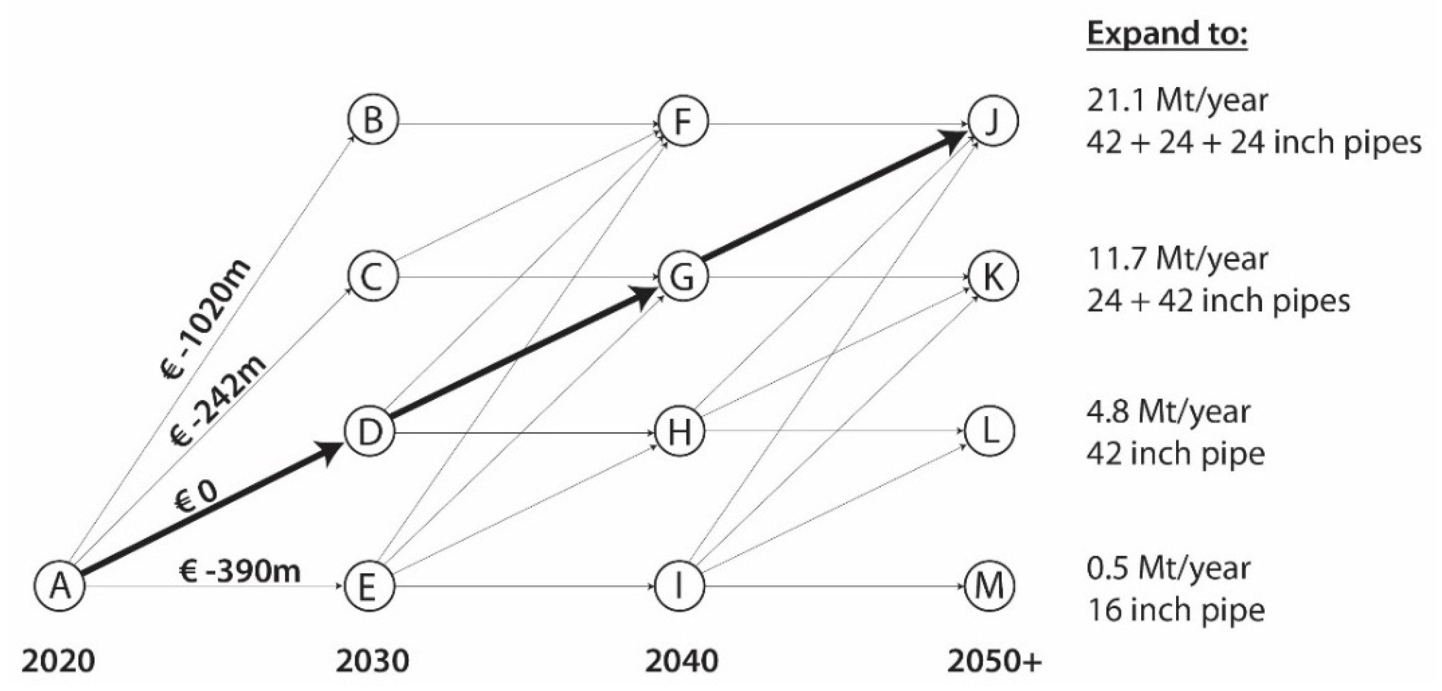
For the case study, the optimal path for the levelized unit price (break-even) are presented in

Table 3. Results for the case study for break-even.

Levelized Unit Costs (EUR/kg/1000 km)	Optimal Path	Sequential Decisions	Pipeline Diameters (Inch)
0.42	$A$–$D$–$G$–$J$	2020: expand to 4.8 Mt/y	42
		2030: expand to 11.7 Mt/y	42 + 24
		2040: expand to 21.1 Mt/y	42 + 24 + 24

and Figure 3. The optimal path reads $A$–$D$–$G$–$J$. It states that for a break-even situation, the most optimal expansion strategy is to expand the current capacity to 4.8 Mt/y, 11.7 Mt/y and 21.1 Mt/y in the years 2020, 2030 and 2040, respectively. Figure 3 shows a generalized rendering of the full decision tree, which enhances the presentation and interpretation of the results. The full decision tree with all options for pipeline diameters as depicted in Table 2 is provided in Appendix A, Figure A1. Both trees are identical, however the tree in Appendix A shows more details.

The levelized costs for hydrogen supply in the current case study are calculated as EUR 0.42 per kilo of hydrogen per 1000 km. This reflects the required average price of hydrogen to cover the minimal life cycle costs of the optimal expansion strategy. In comparison, the levelized costs for hydrogen supply on a European scale in [41] are estimated at EUR 0.09–EUR 0.17 per kilo of hydrogen transported per 1000 km.

Differences are explained by the underlying assumptions on, i.e., purpose, demand development and penalties for missed benefits but also the smaller scale of the current case study plays a role (less economies of scale). Still, values are comparable given the current uncertainty on future hydrogen costs and prices, which provides substantiation for the cost values calculated in the current research by means of [36,41] in Appendix B.

3.2. Sensitivity Analysis

The result indicates the optimal expansion strategy for a break-even situation where the revenues just cover the life cycle costs given the current best estimates for costs, demand development and its uncertainty. The ROA model allows for calculating this levelized unit price for hydrogen by iteration (changing the unit price for hydrogen until the value EUR 0 is reached for the first optimal path). This calculation is now taken as the departing point for the sensitivity of current input values for the optimal path. The scenarios for the sensitivity analysis were constructed with the stakeholders of this research. Questions of interest are primarily related to the impact of the costs of the hydrogen compressors, the uncertainty estimates for demand development, the impact of the unit price of hydrogen and the impact of the penalties (lost income, missed benefits). These aspects were translated into five key questions, which were further detailed within their scope. The five key questions of interest and their summarized answers are depicted in

Table 4. Results of the sensitivity analysis for the case study.

Scenario	Optimal Path	Sequential Optimal Decisions	Pipeline Diameters (Inch)
1. Reduction of compressor costs by 20%	$A$–$D$–$G$–$J$	2020: expand to 4.8 Mt/y	42
		2030: expand to 11.7 Mt/y	42 + 24
		2040: expand to 21.1 Mt/y	42 + 24 + 24
2. Increased likelihood of higher demands by 10%	$A$–$C$–$G$–$J$	2020: expand to 11.7 Mt/y	42 + 24
		2030: remain at 11.7 Mt/y	42 + 24
		2040: expand to 21.1 Mt/y	42 + 24 + 24
3. Increased likelihood of lower demands by 10%	$A$–$D$–$H$–$K$	2020: expand to 4.8 Mt/y	42
		2030: remain at 4.8 Mt/y	42
		2040: expand to 11.7 Mt/y	42 + 24
Unit price income multiplied by 1.5	$A$–$C$–$F$–$J$	2020: expand to 11.7 Mt/y	42 + 24
		2030: expand to 21.1 Mt/y	42 + 24 + 24
		2040: remain at 21.1 Mt/y	42 + 24 + 24
Penalties for lost income reduced by 50%	$A$–$D$–$G$–$J$	2020: expand to 4.8 Mt/y	42
		2030: expand to 11.7 Mt/y	42 + 24
		2040: expand to 21.1 Mt/y	42 + 24 + 24

and Figure 4, and read:

• What is the effect of changes in costs for hydrogen compressors?
  The current high costs of compressors push down the incentives for expansion. The case of 80% of the compressor costs would induce expansion to 11.7 Mt/y. This would alter the current optimal baseline decision.
• What is the effect of high-demand scenarios (11.7 Mt/y and 21.1 Mt/y) becoming more likely in the (near) future?
  If high-demand scenarios increase more than currently foreseen, this will induce incentives for expansion to higher levels on a short notice. A 10% increase of the two high-demand scenarios will change the first optimal expansion decision to 11.7 Mt/y.
• What is the effect of low-demand scenarios (0.5 Mt/y and 4.8 Mt/y) becoming more likely in the (near) future?
  Lower demand than currently foreseen (increased likelihood of occurrence of the low-demand scenarios with 10% to 20%) does not alter the current optimal baseline decision.
• What is the effect of increased income prices per sold hydrogen unit?
  A margin of 50% on the levelized income unit price will induce expansion to 11.7 Mt/y immediately. This would alter the current optimal baseline decision.
• What is the effect of reduced penalties (missed benefits) when demand exceeds the installed capacity?
  A reduction of 50% for the penalties will not alter the current optimal baseline decision. However, if the penalties for lost income are ignored in full, incentives for expansion remain idle.

The results from the sensitivity analysis are confirmed intuitively from a decision maker’s point of view. For example, when compressor costs are reduced, the initial investments are lower, which make earlier expansion to a higher capacity more attractive. In the sensitivity analysis the reduction value was sought for which an alternate path would emerge, being 20%. Likewise, if the expectations for future demand for hydrogen are lowered (resulting in less revenues), the expansion to higher capacities are tempered. In contrast, if the expected future demand is higher than the current expectations, a decision maker would opt for quick expansion to meet that demand. If the penalties for missed income are reduced when demand exceeds capacity installed, it would be more attractive to deploy a conservative strategy and accept income losses. If the price for hydrogen transportation is increased, more revenues will induce quicker expansion. The values of the scenarios of the sensitivity analysis have been chosen to investigate the potential turning points.

The sensitivity analysis may result in confusion because new optimal paths emerge. A decision maker is most interested in the first optimal decision. The decision maker has to weigh the likelihood of the sensitivity scenarios. A reduction of compressor costs in the short term of 20% is not very likely. The scenarios for demand development, as depicted in Table 1, are constructed based on current best expectations, and there is no reason to deviate from them in the short term. The penalties for lost income were chosen with care and are currently considered a reasonable estimate for risk costs. Finally, the unit price is considered. The levelized unit cost for break-even was calculated at 0.42 EUR/kg/1000 km. If the price for transportation would be increased by a factor 1.5 to 0.63 EUR/kg/1000 km, immediate expansion to 11.7 Mt/y would be induced. However, increasing the price may also lower future demand. A decision maker needs to weigh the options. These answers cannot be given by the ROA model or the current research because, here, research into business development is required. However, the ROA model supports asking the right questions and demonstrates the consequences of expectations and potential decisions. It is a tool to support decision making. The decision maker may want to construct some combined sensitivity scenarios. An ROA model supports a quick calculation of numerous sensitivity scenarios and helps the decision maker to evaluate the optimal path from a broader perspective.

The first interest of a decision maker lies in the first optimal decision. The case study provides a preference for $A$–$D$ or $A$–$C$, which is fairly robust. The price for hydrogen transportation seems to be the most decisive factor for the current decision. Therefore, the decision maker will have to investigate this further. For example, subsidy may be attracted to keep the unit price of hydrogen at or below the levelized unit price to stimulate demand. Future decisions can be optimized when progressing in time as current uncertainty will becomes known, and the model can be updated.

3.3. Limitations of the Case Study

Decision making on capital-intensive infrastructure in the Netherlands follows four primary stages: study, exploration, plan elaboration and realization [44]. The current case study aims to support the exploration stage where promising solutions are identified and at the outset are investigated on their feasibility and impact. Feasible solutions are hereafter to be further detailed and evaluated in the design stage. Therefore, this case study is not meant to provide the final answers on hydrogen expansion in the port of Rotterdam.

The ROA analysis has been carried out with great care, but cost values need more refinement in the next stages of decision making. The sensitivity analysis provides focus for further refinement. This will not alter the approach.

The optimal long-term expansion strategy is based upon current best estimates of the hydrogen demand development and its uncertainty, current technical feasible options and their costs and revenues. Such estimates are, by definition, subject to their own uncertainty. These estimates and values can change over time due to technical developments and may influence the optimal expansion strategy. The optimal expansion for hydrogen transport follows from a trade-off between costs and revenues, which builds on scenarios for demand development based on expert judgement. Moreover, calculated compressor capacities need more investigation, especially in relation to a growing hydrogen demand. New technology probably will be introduced, reducing compressor costs. Additionally, other aspects of the pipelines, such as the thickness of the walls and the number of compressor stations, have not yet been included in the calculation.

4. Discussion

First, this section discusses the methodological variations in the ROA applications found in the literature. This motivates the choices that were made for the current case study modelling approach. Moreover, it motivates why the current modelling approach adds to the scientific body of knowledge. Hereafter, the discussion is continued from the perspective of the stakeholders of the current research whose interest lies in the application of ROA in professional practice.

4.1. Discussion from a Methodological Perspective

ROA for decision making under uncertainty has attracted the attention of numerous scholars. The scientific literature offers a broad array of ROA applications among a broad array of domains such as flood defense [45,46], water supply [47,48], infrastructure maintenance and replacement [49,50], construction and public–private partnerships [24,51,52,53,54,55], exploitation of toll roads [56] and the energy sector [14,15,16,26]. Over the last years, ROA has quickly emerged in the literature on energy transition, firstly because energy transition is subject to uncertainty and rapidly changing environments and secondly because valuing flexibility can make innovative but expensive investments attractive, whereas traditional discounted cash flow would not [14,20,27].

While comparing ROA applications, the differences are seen in the purpose of the ROA, the number of uncertainties incorporated, the uncertainty quantifications, the ROA option valuation method and whether an ROA is two-staged (two options) or compound (successive multiple options). It may be clear that these characteristics are case-specific, which explains the wide variety of ROA applications.

The literature can be classified in two-staged ROA applications and compound ROA applications. Two-staged ROA applications have two options, generally to wait or invest and incorporate one or more uncertainty variables such as demand development or prices. In contrast, compound ROA applications have multiple options which progress in time [16,25,27,57]. Previous decisions lead to new options and compound ROAs optimize a sequence of decisions under one or more underlying uncertainty variables. Two-staged ROA applications are well represented in the literature, whereas the literature is far less rich and even shallow on compound ROA applications [16].

Reviewing the literature, the following observations emerge. First, most ROA applications are single timing-options: two-staged ROAs such as wait or invest. The complexity in these ROA applications is seen in the uncertainty quantification. Most single timing-options models opt for the inclusion of multiple uncertainties [15,20,26,49]. A GBM is often used to simulate future prices, but stochastic Arithmetic Brownian Motion, ARIMA or GARCH processes have also been observed in the literature. Although GBM is popular, it is also criticized for being inadequate for the prediction of prices in real projects [19,29,31,32]. Most researchers use historic data and expert judgement to estimate the parameters that describe stochastic processes or probability density functions. This shows that the availability of data influences the approach to uncertainty quantification, which explains why different researchers make different choices.

Second, the inclusion of multiple uncertainties in the literature is mostly tied to single investment-timing options (two-staged ROAs). Because of the limitation to two repetitive options (invest or wait), the independent time-variant uncertainties can easily be combined with a Monte Carlo Simulation. This results in thousands of simulations but just two outputs: an optimal timing and an optimal option value.

However, in compound ROAs with multiple successive options (expansion strategy), a decision maker is interested in the time-variant strategy or the optimal sequence of decisions and the impact of the uncertainty variables. Monte Carlo simulations easily combine multiple uncertainties but also function as a black-box approach, as they do not easily provide the optimal sequence of compound decisions nor the impact of uncertainty variables on the optimal path. In contrast to this, a compound ROA application, with four underlying uncertainty variables without using Monte Carlo simulations, is provided by [27]. Instead, discrete backward induction is applied. This approach makes it in possible to trace the optimal expansion strategy. However, the inclusion of multiple uncertainty variables also exponentially enlarges the underlying decision tree. The authors present a decision tree with 390 × 76,050 nodes for their case study. Tracing an optimal expansion strategy and comparison with alternate paths is challenging in such large trees. It is observed that this was not the objective of these authors. Their model is fit for their purpose: to provide an ROA option value for an optimal strategy.

The expansion of a hydrogen network in the Port of Rotterdam also faces this dilemma of the so-called Bellman’s curse of multi-dimensionality [58]. At each decision node, there are multiple options to expand a pipeline network to a certain capacity, but the options also depend on previous options, and the best option in each state depends on the value taken by the uncertainty variables. A closed-form option value calculation will not provide a clear visual strategy as it is a black-box approach. In contrast, an open-form ROA calculation visualizes an optimal strategy in a decision tree. However, it cannot properly handle the inclusion of multiple uncertainties because the tree will expand exponentially. The current study proposes an approach to handle this dilemma through the inclusion of one dominant uncertainty variable in the ROA calculation. The impact of other uncertainty variables is investigated afterwards with a sensitivity analysis.

A third observation emerging from the literature is that uncertainty quantification is often built on the analysis of historic data. However, historic data are not always available, and especially not when dealing with new technologies such as hydrogen supply. In the literature, it is observed that scenarios are used for uncertainty quantification in the absence of data. Moreover, the authors of this research are inspired by the use of the aggregated levelized costs by [20] based on analysis of historic data. However, future prices of hydrogen are uncertain and cannot be predicted based on historic data. In contrast to electricity, there are no sector-wide aggregated levelized costs for hydrogen. However, given the absence of historic prices, and given the uncertainty of future hydrogen prices, a compound ROA can also be used to find the case-specific levelized unit price of hydrogen to cover the life cycle cost of the optimal strategy. From there, the impact of other uncertainty variables can be further explored.

The current research adds to body of scientific literature by developing a compound ROA application for the expansion of a hydrogen pipeline network instead of a single investment-timing ROA. The time-variant options rely on previous decisions and are not repetitive. Moreover, the current research uses an open-form approach to the ROA option value calculation because emphasis is put on visualizing an optimal strategy to facilitate decision making. This approach asks for a trade-off with the inclusion of uncertainty variables. The current research has selected future demand as the prime uncertainty variable for inclusion in the ROA. The other uncertainty variables are investigated with a sensitivity analysis afterwards. Finally, as the price of hydrogen is uncertain and impossible to substantiate with historic data, the second purpose of the ROA is to find the case-specific levelized unit price to cover the life cycle costs of the optimal strategy.

4.2. Discussion from a Decision Maker’s Perspective

Real options analysis supports decision making under uncertainty and values flexibility. The current research applied ROA on the expansion of a hydrogen pipeline network in the port of Rotterdam. In this section, the application of ROA is discussed from the perspective of the stakeholders of this research.

4.2.1. ROA Is Part of a Larger Strategy

An ROA is a means to a purpose: In this research, the purpose is developing a long-term adaptive strategy. An effective strategy embeds an ROA and details all steps required for its implementation. In other words, ROA is part of a larger decision-making process where quantitative and qualitative criteria need to be considered. The authors of [17] propose an interesting approach to embed the results of an ROA in an advanced type of multi-criteria analysis to obtain an aggregated quality score. As such, distinct adaptive strategies or different projects with their own underlying ROAs can be compared. In addition to the actual execution, this also entails that parameter and model uncertainties need to be monitored and regularly updated.

4.2.2. ROA Needs to Be Fit for Purpose

ROA needs case-specific modelling where context is key. This context is provided by experts and stakeholders but also by the availability of data.

Some major challenges in an ROA are how to identify the most dominant uncertainties, how to quantify uncertainties and how to combine uncertainties while keeping results explainable. In the case study for hydrogen expansion, one uncertainty variable was chosen: the development of demand. The other uncertainties, for example, on costs, were investigated with a sensitivity analysis afterwards. These choices were made deliberately considering the purpose and context.

Integrating too many uncertainties in an ROA quickly leads to overfitting: a model and results which are difficult to interpret or have become a black-box for decision makers. Overfitting leads to very complex decision trees and requires large computational power for the option value calculations. These models may also induce a false sense of accuracy. The challenge for the application of ROA in practice is describing a complex reality as a model that is as uncomplicated as possible, and which is accurate enough to provide meaningful decision-making information. Results need to be explainable to management.

Considering the data availability, the following was learned. As of today, expert judgement is still common ground for the quantification of many uncertainty variables in practice. Structured methods to support expert judgement are available and may support uncertainty quantification. If appropriate, trend analysis of historic data and forecasting may add to the substantiation of uncertainty quantification.

The current research did not use these more advanced methods for uncertainty quantification. However, it was learned that existing information is underutilized and exploitable. Nowadays, many open data are available in various sources. Finding, judging and combining these pieces of information, together with professional experts, also leads to the substantiation of uncertainty quantification.

4.2.3. ROA Needs Cost Data of Future Options

ROA needs cost data of all future options. The costs (and revenues) of each path in a decision tree need to be estimated and discounted to a local departing node. This can be time-consuming if decision trees are not compact. Moreover, future costs are by definition uncertain, and it raises the question of how to deal with this price uncertainty without further complicating the ROA model.

The current case study opted for a sensitivity analysis afterwards on cost data, which may be a good solution to keep ROA models compact. It is, again, a balance. Cost data (prices) could have been treated as an uncertainty variable such as demand, but this would have severely enlarged the model and complicated its interpretability. For the costs, a good insight into the impact of their fluctuations was well obtained by a sensitivity analysis. Still, obtaining sensible cost data for future options is time-consuming and should not be underestimated.

4.2.4. Distinguish Decisions and Uncertainties in a Visual Representation

Decision trees in ROA are visually well understood, if not too complex. Care, however, is required in distinguishing options (subject to decisions, a choice) and uncertainties (what happens beyond control, a chance). Decision trees generally represent options with arrows going from one decision node to another. Uncertainty is not necessarily visible in a tree, which may give rise to confusion. Uncertainty can be embedded visually by introducing additional chance nodes (next to decision nodes), but this will increase the complexity of the visual representation as it enlarges the tree exponentially.

5. Conclusions

Real options analysis (ROA) facilitates adaptive decision making and adds value because it accounts for uncertainty and adds flexibility to enhance future decisions. The current research applied a multi-staged ROA to find the optimal expansion strategy for a hydrogen pipeline network in the port of Rotterdam under uncertain demand development. When installed capacity exceeds demand, unnecessary investments were made. When demand exceeds installed capacity, potential income is lost. Phased expansion minimizes these risks.

The ROA is first used to find the case-specific levelized unit price for hydrogen supply. This is the required unit price for hydrogen to cover the life cycle costs of the optimal expansion strategy under uncertain demand. Departing from here, the impact of uncertainty variables is further investigated. The ROA provides visual optimal paths for expansion and offers flexibility to enhance future decisions.

The case study needs further refinement.

Barriers are also found. ROA requires case-specific modelling and choosing the right uncertainty variables is challenging. Too-simple ROA models may not provide accurate decision-making information because of omission of data, and too-complex ROA models may provide a false sense of security because of overfitting with inadequate data. Combining multiple uncertainties may also lead to results which are perceived as a black-box by decision makers.

The case study aims to balance complexity and simplicity. This is a strength but may also be a weakness. As for further research, we propose to investigate the cost values and their uncertainty more in depth. The sensitivity analysis shows that the price of hydrogen transportation may be decisive for the best current expansion strategy. However, price is known to have a relation with demand. Stimulating hydrogen demand may require lower prices or additional subsidy. The relation between demand development and price needs further investigation. In addition, the financing of investments, which may influence the unit price, needs further research. Moreover, the probabilities for demand development are based on expert judgment with a few stakeholders. This can be improved by expansion of experts to be consulted and by the application of structured methods to elicit expert judgement.

From an academic perspective, the current research adds an approach for a compound ROA (multi-staged) with multiple dependent unique options while preserving a visual representation of an optimal path. The trade-off is in the limitation to one underlying uncertainty variable for demand development. The uncertainty of other variables is investigated afterwards with a sensitivity analysis.

Furthermore, the current research emphasizes that ROA applications should always be embedded in a larger strategy to operationalize its results.