
Statistical Modelling of the Market Value of Dwellings, on the Example of the City of Kraków


Abstract
:1. Introduction
2. Materials and Methods
2.1. Multidimensional Regression
- small changes in the database result in large changes in the value of estimators;
- regression equation coefficients have large standard deviations, thus they may be statistically insignificant, despite even a high R2 determination factor (together they are relevant).
2.2. Rule of Thumb
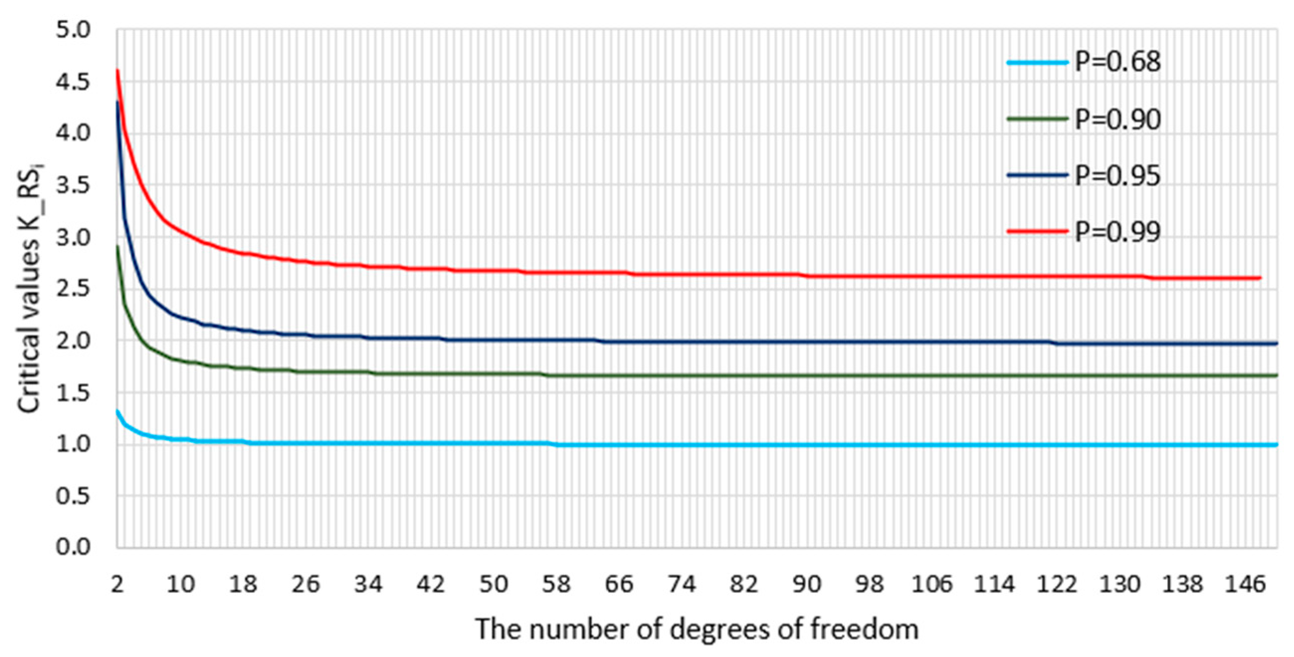
2.3. Mahalonobis Distance
- —Mahalonobis Distance,
- —a vector containing the ith explanatory variables,
- —vector of the average explanatory variables,
- —covariance matrix for explanatory variables.
- n—number of observations,
- —the value of leverage for the first observation.
2.4. Analysis of Standardized Model Residuals
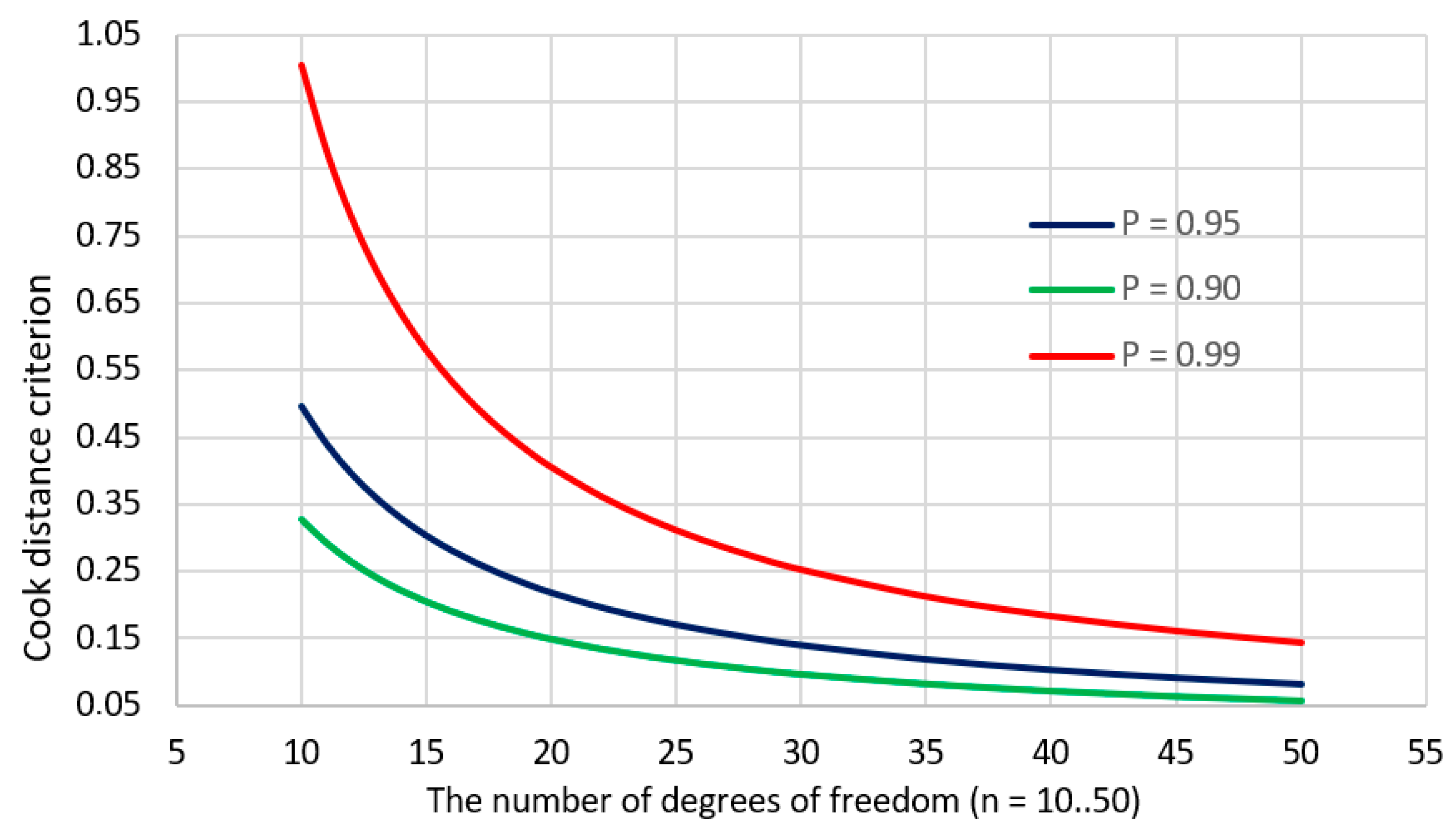
2.5. Cook’s Distance
- —Cook’s distance,
- —variance estimator calculated based on all observations,
- —an estimator of variance calculated after elimination of the first observation,
- n—number of observations,
- u—number of model parameters.
- —the value predicted by the model for the jth observation determined in the full model,
- —the value predicted by the model for the jth observation determined based on the model from which the ith observation was removed.
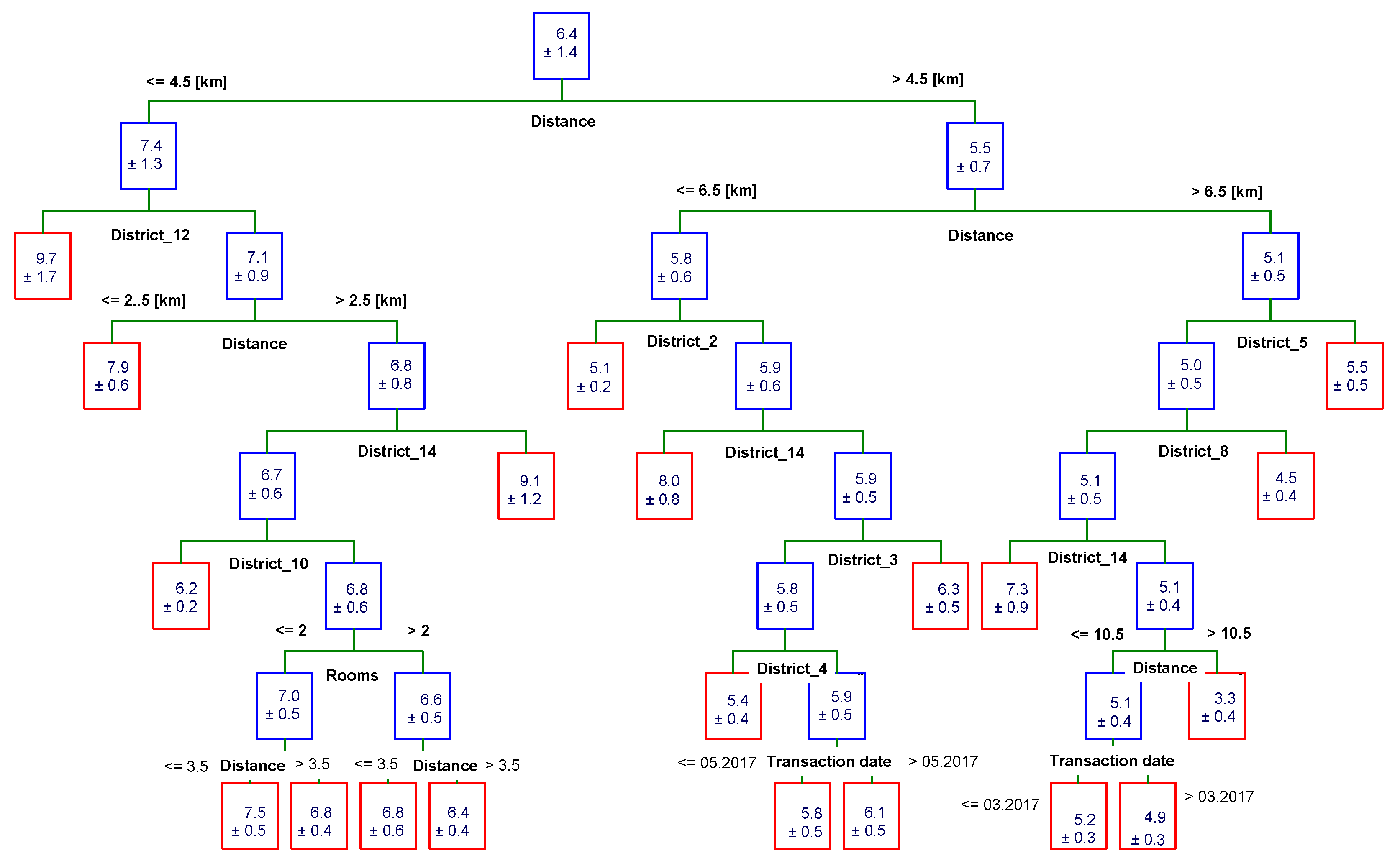
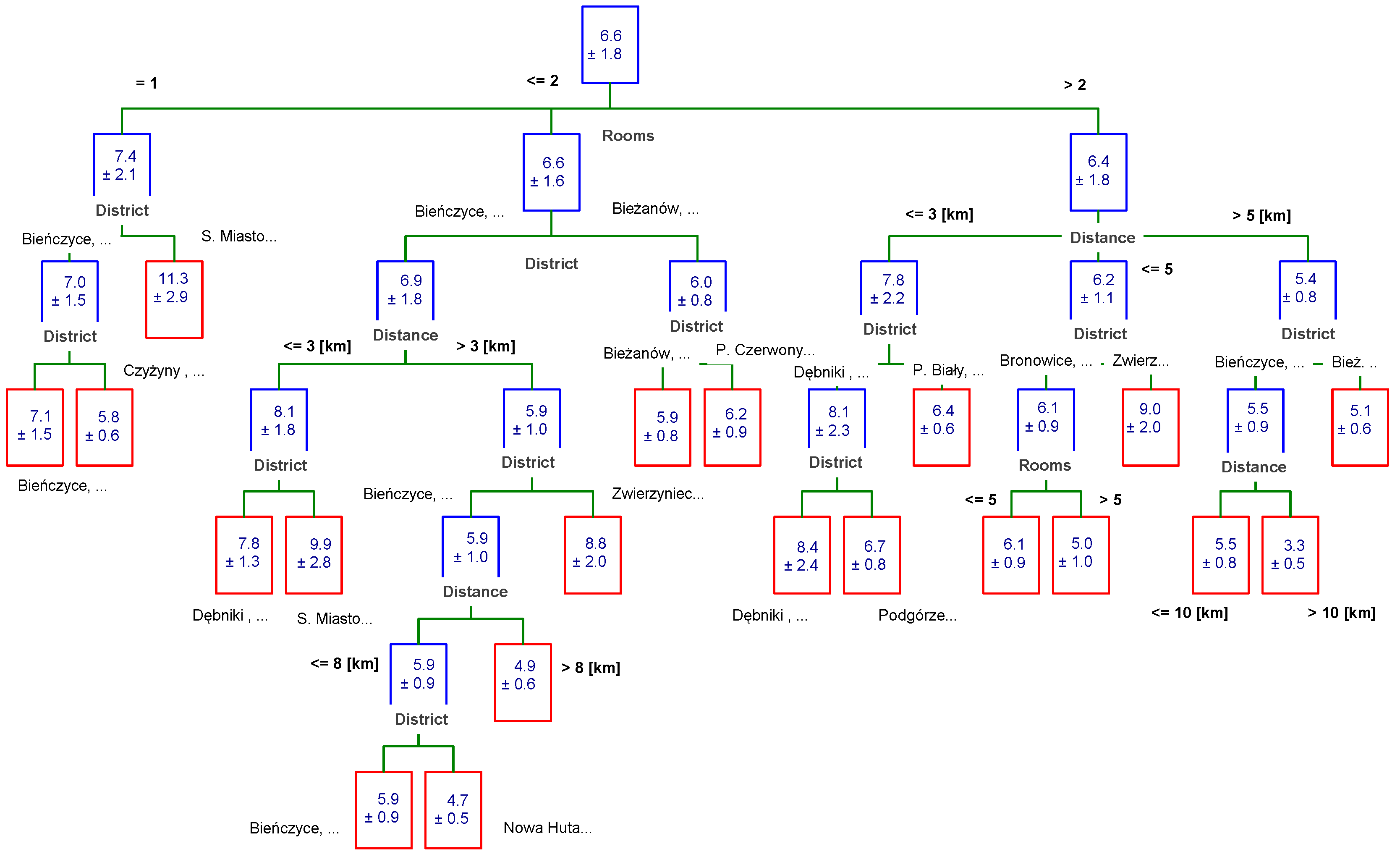
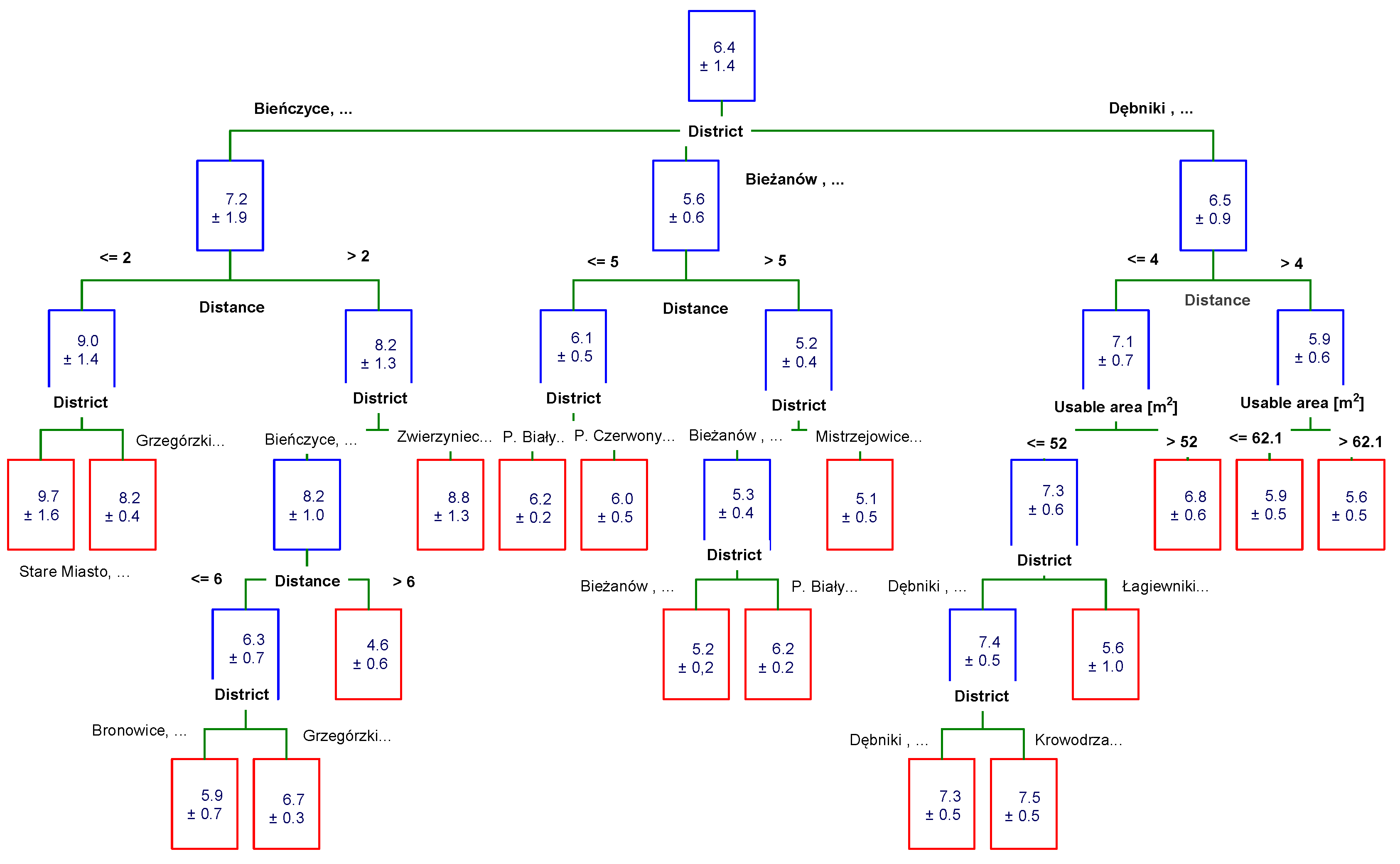
2.6. Classification and Regression Tree Models
- Tree building: the process occurs through the recursive division of nodes,
- Stopping the construction of the tree: at this stage, the tree is as extensive as possible, usually containing redundant information,
- Pruning of the tree consists of removing redundant branches,
- Choosing the right tree: some branches are restored to increase the effectiveness of the method.
3. Results
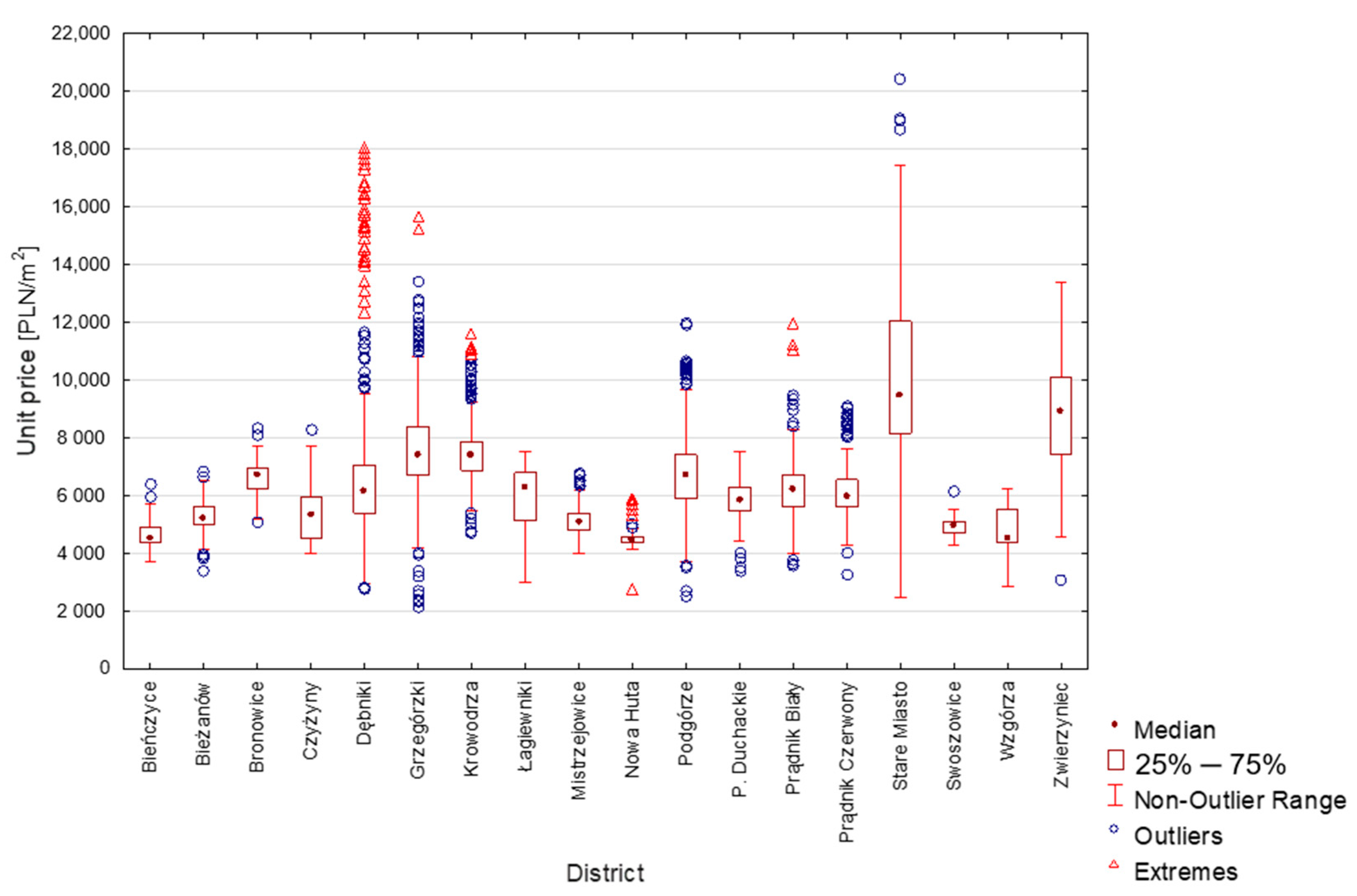
3.1. Identification of Influential and Outliers in the Kraków Database
3.2. Multidimensional Regression Models for Kraków Databases
3.3. C&RT Trees
- variable dependent—unit price,
- quality predictors—district,
- quantitative predictors—distance, area, floor, transaction date,
- minimum number in the end node: 20.
3.4. Chi-Square Automatic Interaction Detector (CHAID) Trees
4. Conclusions
Author Contributions
Funding
Institutional Review Board Statement
Informed Consent Statement
Data Availability Statement
Acknowledgments
Conflicts of Interest
References
- Marona, B.; Tomal, M. The COVID-19 pandemic impact upon housing brokers’ workflow and their clients’ attitude: Real estate market in Krakow. Entrep. Bus. Econ. Rev. 2020, 8, 221–232. [Google Scholar]
- Kowalczyk-Anioł, J.; Grochowicz, M.; Pawlusiński, R. How a Tourism City Responds to COVID-19: A CEE Perspective (Kraków Case Study). Sustainability 2021, 13, 7914. [Google Scholar] [CrossRef]
- Kilpatrick, J.A. The future of real estate information. Real Estate Issues 2001, 26, 7–14. [Google Scholar]
- Romańczyk, K. Krakow—The City Profile Revisited; Elsevier: New York, NY, USA, 2018; Volume 73. [Google Scholar]
- Available online: https://pl.wikipedia.org/wiki/Podzia%C5%82_administracyjny_Krakowa (accessed on 23 July 2021).
- Zyga, J. Evaluation of usefulness of real estate data contained in the register of prices and values of real estates. Infrastrukt. Ekol. Teren. Wiej. 2017. [Google Scholar] [CrossRef]
- Halik, Ł. Analysis of County Geoportals in Terms of Opportunities to Purchase Data of the Register of Real Estate Prices and Values Online. Real Estate Manag. Valuat. 2019, 27, 69–78. [Google Scholar] [CrossRef] [Green Version]
- Halik, Ł. Information and Communication Systems Used for Keeping the Register of Real Estate Prices and Values (Rrepv) in Poland. Real Estate Manag. Valuat. 2018, 26, 45–53. [Google Scholar] [CrossRef] [Green Version]
- Kannan, K.S.; Manoj, K. Outlier Detection in Multivariate Data. Appl. Math. Sci. 2015, 9, 2317–2324. [Google Scholar] [CrossRef]
- Preweda, E. Outlier detection in surveying networks. In Proceedings of the 14th International Multidisciplinary Scientific Geoconference (SGEM), Albena, Bulgaria, 17–26 June 2014; Volume 2, pp. 365–372. [Google Scholar]
- Crecente, R.; Alvarez, C.; Fra, U. Economic, social and environmental impact of land consolidation in Galicia. Land Use Policy 2002, 19, 135–147. [Google Scholar] [CrossRef]
- Wójcik-Leń, J.; Leń, P.; Mika, M.; Kryszk, H.; Kotlarz, P. Studies regarding correct selection of statistical methods for the needs of increasing the efficiency of identification of land for consolidation—A case study in Poland. Land Use Policy 2019, 87, 104064. [Google Scholar] [CrossRef]
- Greene, W.H. Econometric Analysis, 5th ed.; Prentice Hall: Upper Saddle River, NJ, USA, 2003. [Google Scholar]
- Mahalanobis, P.C. On the Generalised Distance in Statistics. Proc. Natl. Inst. Sci. India 1936, 2, 49–55. [Google Scholar]
- Ghorbani, H. Mahalanobis Distance and Its Application For Detecting Multivariate Outliers. Facta Univ. Ser. Math. Inform. 2019, 34, 583–595. [Google Scholar] [CrossRef]
- Cook, R.D. Detection of Influential Observations in Linear Regression. Technometrics 1977, 19, 15–18. [Google Scholar]
- Zhu, H.; Ibrahim, J.G.; Cho, H. Perturbation and scaled Cook’s distance. Ann. Stat. 2012, 40, 785–811. [Google Scholar] [CrossRef] [Green Version]
- Vukovic, O. Analysing bank real estate portfolio management by using impulse response function, Mahalanobis distance and financial turbulence. Procedia Econ. Financ. 2015, 30, 932–938. [Google Scholar] [CrossRef] [Green Version]
- Stöckl, S.; Hanke, M. Financial applications of the Mahalanobis distance. Appl. Econ. Financ. 2014, 1, 78–84. [Google Scholar] [CrossRef] [Green Version]
- Jung, E.; Yoon, H. Is Flood Risk Capitalized into Real Estate Market Value? A Mahalanobis-Metric Matching Approach to the Housing Market in Gyeonggi, South Korea. Sustainability 2018, 10, 4008. [Google Scholar] [CrossRef] [Green Version]
- Isakson, H.R. Valuation analysis of commercial real estate using the nearest neighbors appraisal technique. Growth Chang. 1988, 19, 11–24. [Google Scholar] [CrossRef]
- Chen, W.; Xie, X.; Wang, J.; Pradhan, B.; Hong, H.; Bui, D.T.; Duan, Z.; Ma, J. A comparative study of logistic model tree, random forest, and classification and regression tree models for spatial prediction of landslide susceptibility. Catena 2017, 151, 147–160. [Google Scholar] [CrossRef] [Green Version]
- Herath, S.; Maier, G. The Hedonic Price Method in Real Estate and Housing Market Research: A Review of the Literature; SRE-Discussion Papers, 2010/03; WU Vienna University of Economics and Business, Vienna, Austria, 31 March 2010. Available online: https://ideas.repec.org/p/wiw/wus009/588.html (accessed on 1 August 2021).
- Janssen, C.; Söderberg, B.; Zhou, J. Robust estimation of hedonic models of price and income for investment property. J. Prop. Invest. Financ. 2001, 19, 342–360. [Google Scholar] [CrossRef]
- Bourassa, S.C.; Cantoni, E.; Hoesli, M. Robust hedonic price indexes. Int. J. Hous. Mark. Anal. 2016, 9, 47–65. [Google Scholar] [CrossRef]
- Mok, H.M.K.; Chan, P.P.K.; Cho, Y.S. A hedonic price model for private properties in Hong Kong. J. Real Estate Financ. Econ. 1995, 10, 37–48. [Google Scholar] [CrossRef]
- Chau, K.W.; Chin, T.L. A Critical Review of Literature on the Hedonic Price Model (12 June 2002). Int. J. Hous. Sci. Appl. 2003, 27, 145–165. [Google Scholar]
- Scott, D.W. Partial Mixture Estimation and Outlier Detection in Data and Regression. In Theory and Applications of Recent Robust Methods; Birkhauser: Basel, Switzerland, 2014; pp. 297–306. [Google Scholar] [CrossRef] [Green Version]
- Rao, C.R.; Toutenburg, H. Linear models. In Linear Models; Springer: New York, NY, USA, 1995; pp. 3–18. [Google Scholar]
- Casson, R.J.; Farmer, L.D. Understanding and checking the assumptions of linear regression: A primer for medical researchers. Clin. Exp. Ophthalmol. 2014, 42, 590–596. [Google Scholar] [CrossRef] [PubMed]
- Frukacz, M.; Popieluch, M.; Preweda, E. Real Estate Price Adjustment Due to Time in the Case of Large Databases; Infrastructure and Ecology of Rural Areas; Committee on Technical Rural Infrastructure: Krakow, Poland, 2011; pp. 213–226. ISBN 1732-5587. [Google Scholar]
- Jasińska, E. Real estate due diligence on the example of the polish market. In Proceedings of the 14th International Multidisciplinary Scientific Geoconference (SGEM), Albena, Bulgaria, 17–26 June 2014; Volume 2, pp. 419–426. [Google Scholar]
- ScienceDirect Homepage. Available online: https://www.sciencedirect.com/topics/engineering/mahalanobis-distance (accessed on 20 November 2020).
- Algur, S.P.; Biradar, J.G. Cooks Distance and Mahanabolis Distance Outlier Detection Methods to identify Review Spam. Int. J. Eng. Comput. Sci. 2017, 6, 21638–21649. [Google Scholar] [CrossRef]
- Jasińska, E. Chosen Statistical Method in Real Estate Market Analysis; Wydawnictwa Akademii Górniczo-Hutniczej im; Stanisława Staszica w Krakowie: Krakow, Poland, 2012; ISBN 978-83-7464-471-6. [Google Scholar]
- Ho, W.K.O.; Tang, B.-S.; Wong, S.W. Predicting property prices with machine learning algorithms. J. Prop. Res. 2020, 38, 48–78. [Google Scholar] [CrossRef]
- Levantesi, S.; Piscopo, G. The Importance of Economic Variables on London Real Estate Market: A Random Forest Approach. Risks 2020, 8, 112. [Google Scholar] [CrossRef]
- Jasińska, E.; Preweda, E. The use of regression trees to the analysis of real estate market of housing. In Proceedings of the 13th International Multidisciplinary Scientific Geoconference (SGEM), Albena, Bulgaria, 16–22 June 2013; Volume 2, pp. 503–508. [Google Scholar]
- Buntine, W. Learning classification trees. Stat. Comput. 1992, 2, 63–73. [Google Scholar] [CrossRef] [Green Version]


| Number of Properties | Average Unit Price [PLN/m2] | Median [PLN/m2] | Min. Unit Price [PLN/m2] | Max. Unit Price [PLN/m2] | Standard Deviation [PLN/m2] | |
|---|---|---|---|---|---|---|
| Bieńczyce | 70 | 4662 | 4535 | 3733 | 6383 | 474 |
| Bieżanów | 711 | 5273 | 5210 | 3400 | 6805 | 478 |
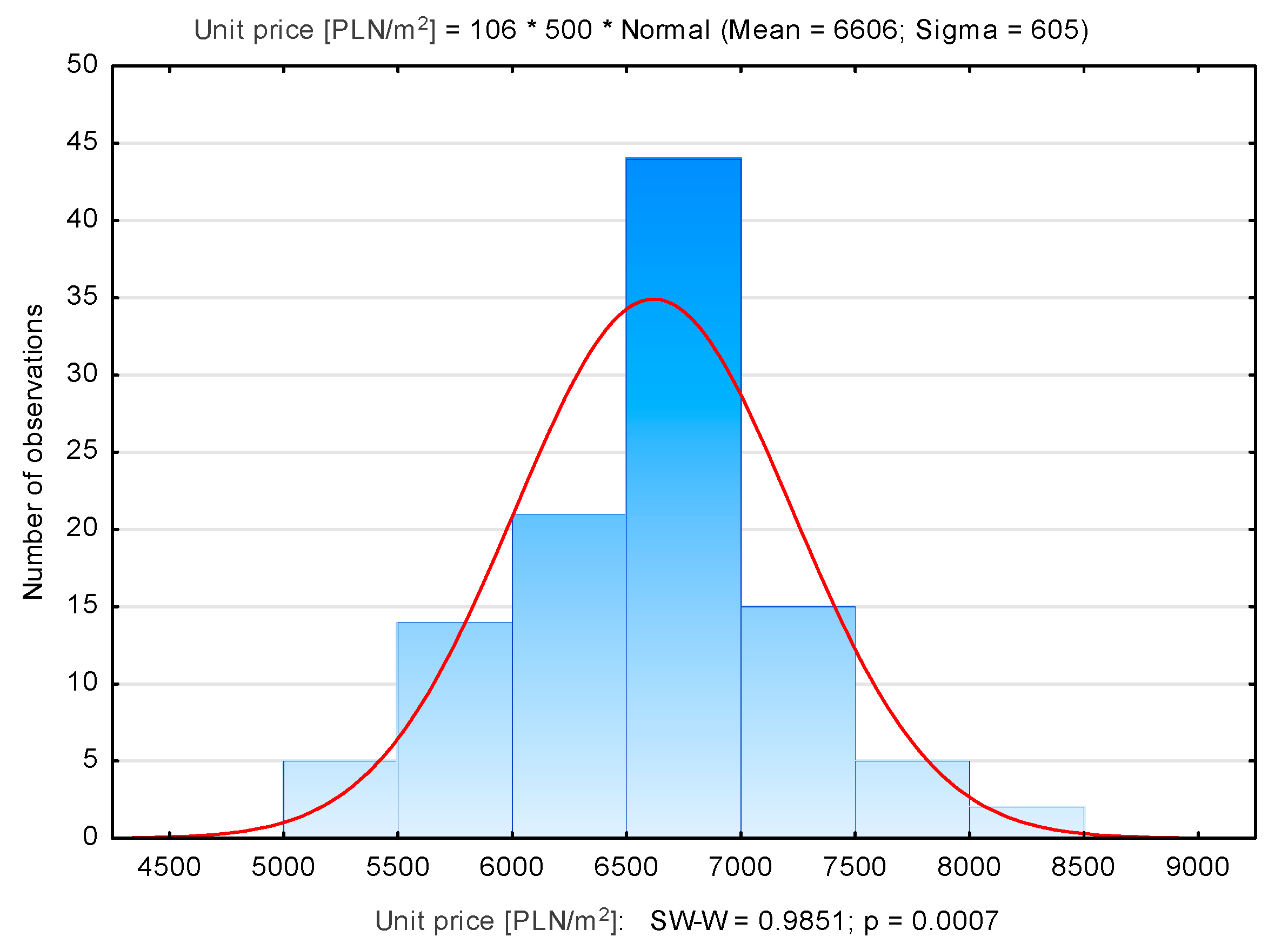
| Bronowice | 106 | 6606 | 6718 | 5054 | 8321 | 605 |
| Czyżyny | 1029 | 5356 | 5311 | 3999 | 8279 | 813 |
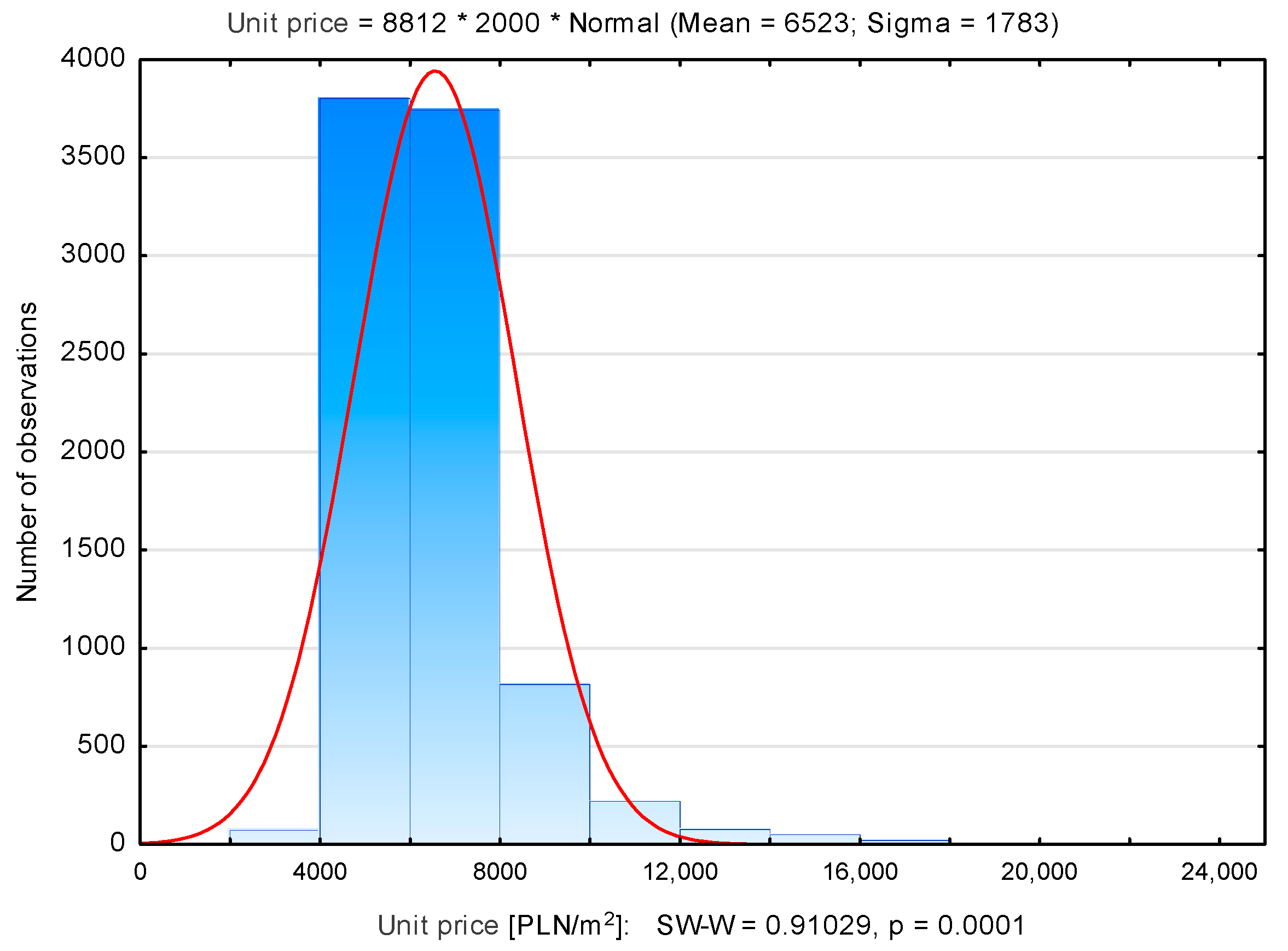
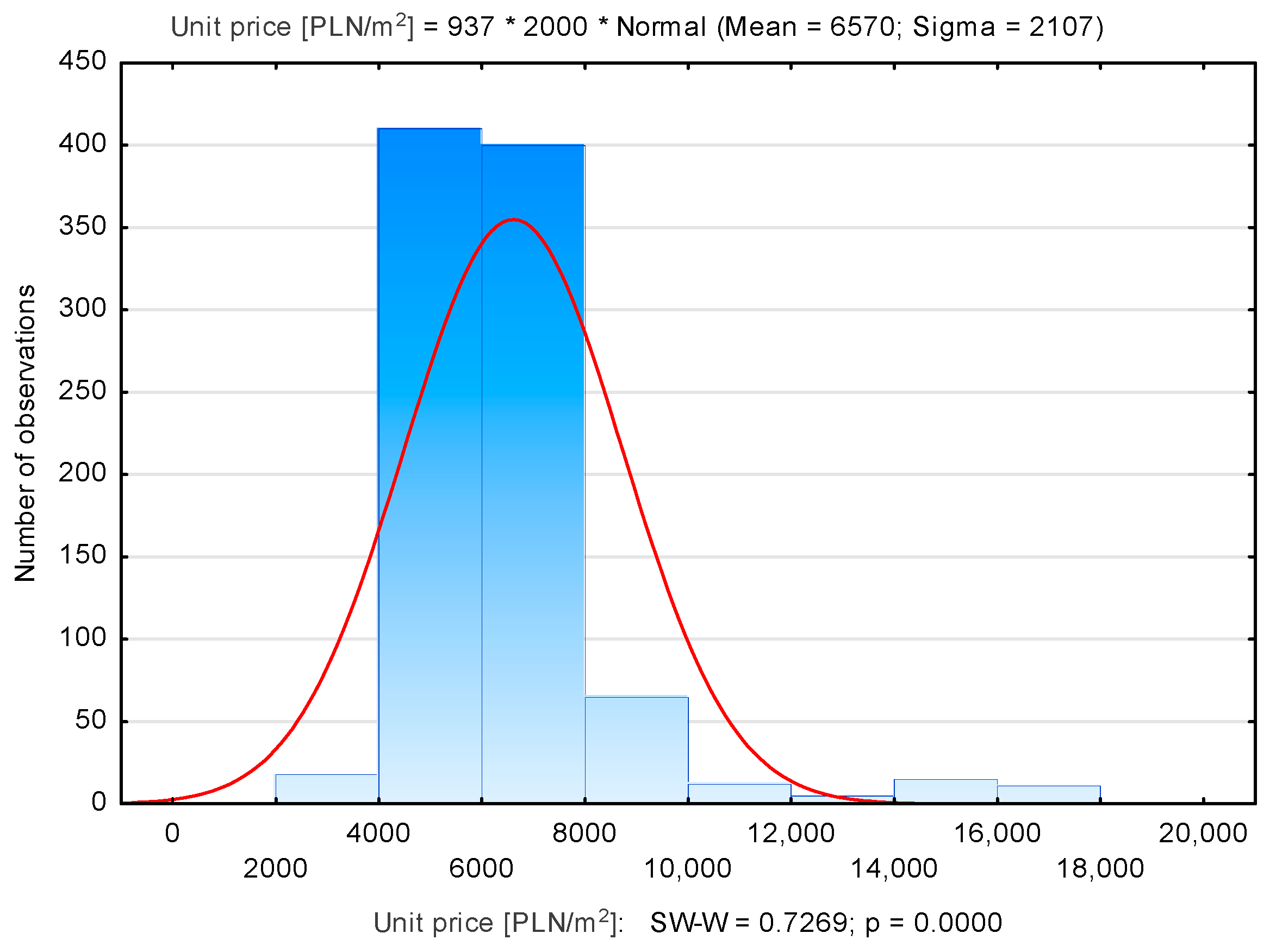
| Dębniki | 937 | 6570 | 6173 | 2790 | 18,043 | 2107 |
| Grzegórzki | 1281 | 7634 | 7395 | 2166 | 15,688 | 1459 |
| Krowodrza | 464 | 7527 | 7389 | 4736 | 11,629 | 1015 |
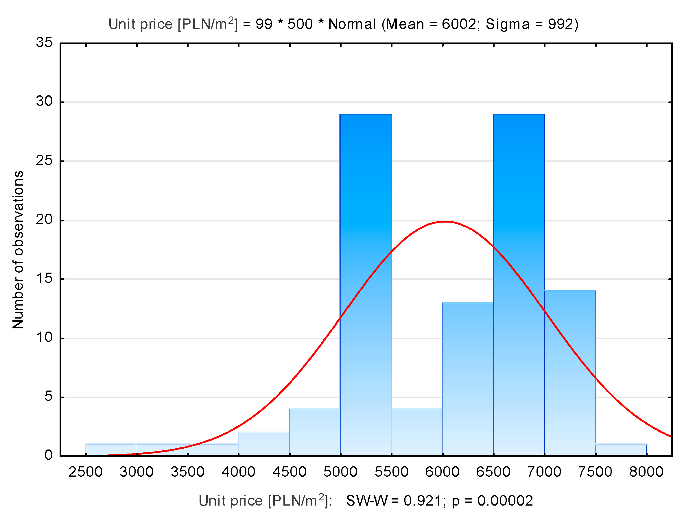
| Łagiewniki | 99 | 6002 | 6246 | 2990 | 7516 | 992 |
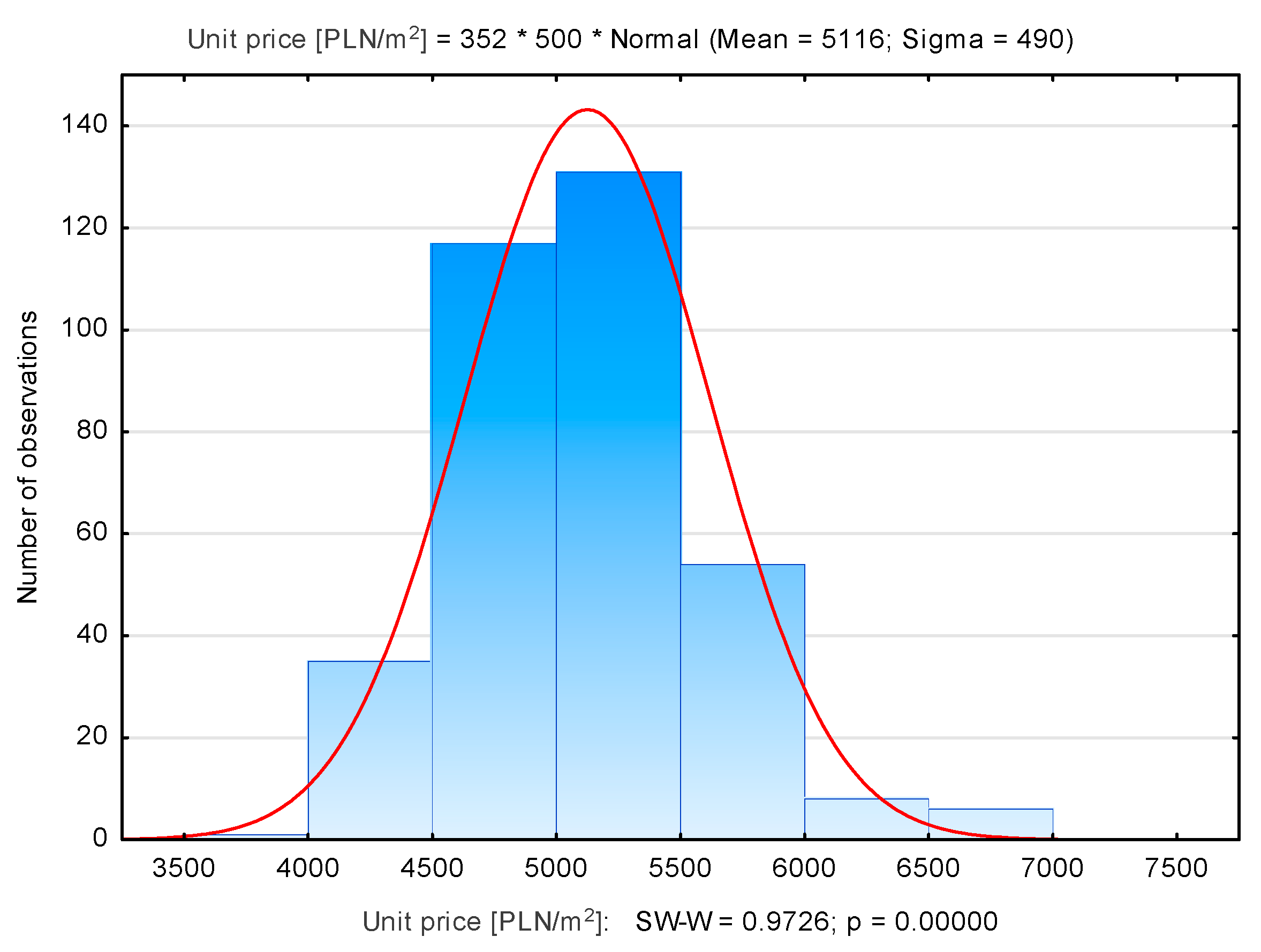
| Mistrzejowice | 352 | 5116 | 5096 | 3999 | 6799 | 490 |
| Nowa Huta | 94 | 4507 | 4466 | 2735 | 5921 | 432 |
| Podgórze | 996 | 6787 | 6712 | 2510 | 11,979 | 1302 |
| P. Duchackie | 360 | 5855 | 5826 | 3367 | 7511 | 593 |
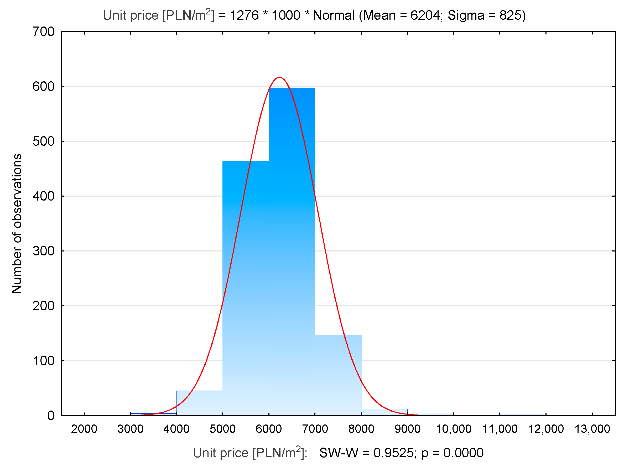
| Prądnik Biały | 1276 | 6204 | 6221 | 3585 | 12,006 | 825 |
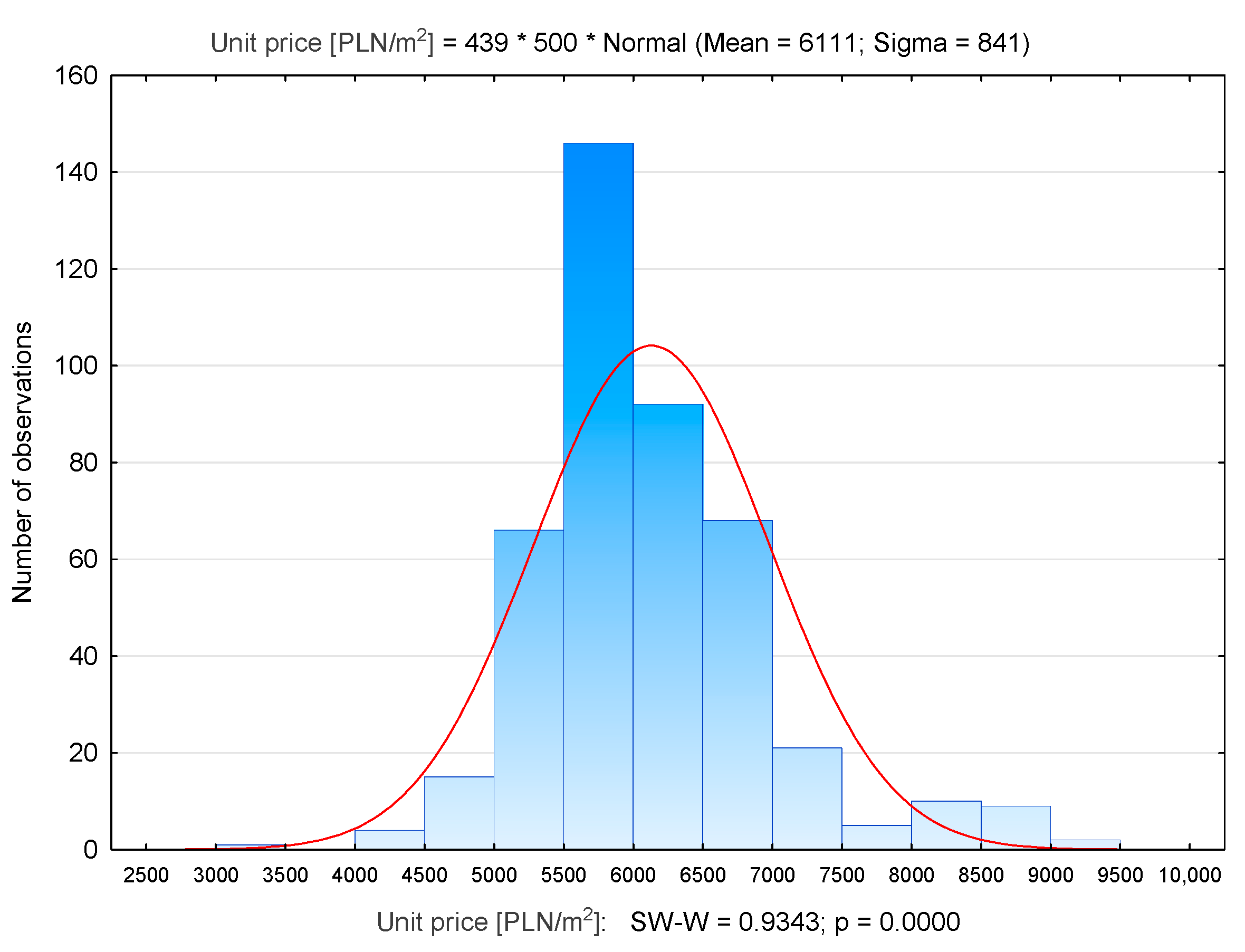
| Prądnik Czerwony | 439 | 6111 | 5962 | 3276 | 9100 | 841 |
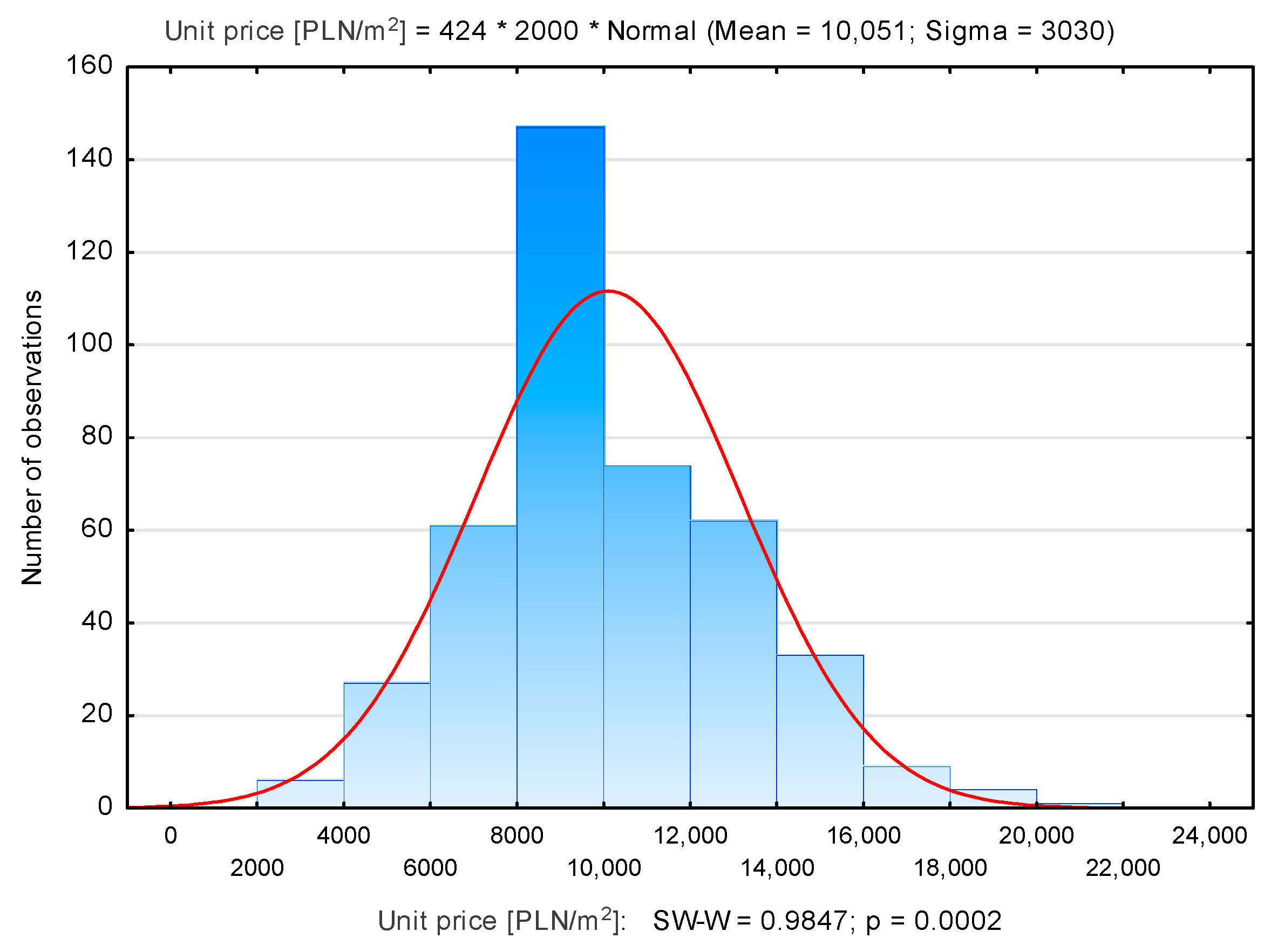
| Stare Miasto | 424 | 10,051 | 9473 | 2467 | 20,446 | 3030 |
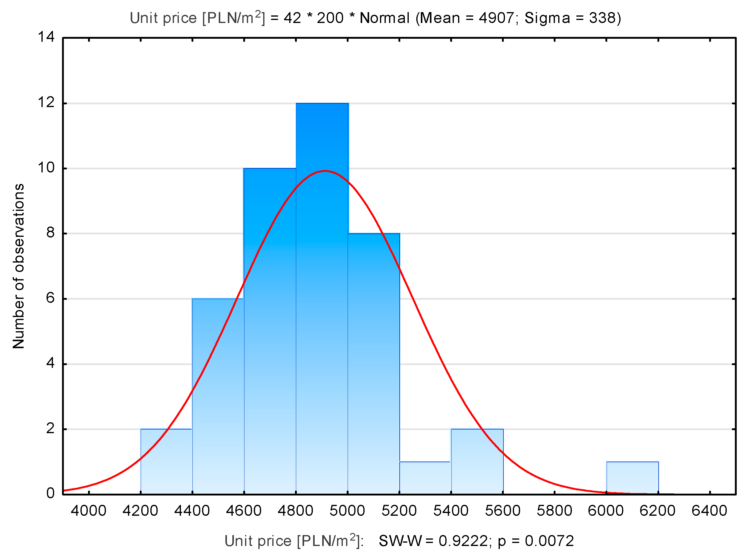
| Swoszowice | 42 | 4907 | 4951 | 4298 | 6170 | 338 |
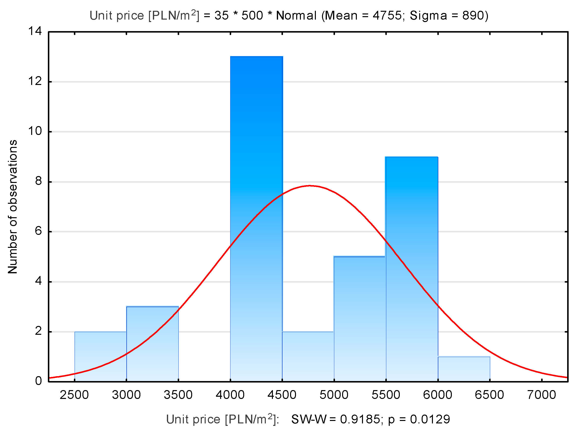
| Wzgórza K. | 35 | 4755 | 4490 | 2853 | 6258 | 890 |
| Zwierzyniec | 97 | 8709 | 8888 | 3100 | 13,393 | 1926 |
| Object | R2 | σ | Distance | Usable Area | Storey | Rooms | Transaction Date |
|---|---|---|---|---|---|---|---|
| Bieńczyce | 0.04 | 471 | - | −0.090 | −0.550 | −0.120 | −0.330 |
| Bieżanów | 0.11 | 451 | 0.234 | −0.030 | 0.279 | −0.160 | −0.180 |
| Bronowice | 0.28 | 522 | −0.450 | 0.150 | 0.150 | −0.310 | 0.119 |
| Czyżyny | 0.29 | 612 | −0.380 | 0.457 | 0.061 | −0.680 | −0.160 |
| Dębniki | 0.45 | 1577 | −0.550 | 0.387 | 0.071 | −0.150 | 0.061 |
| Grzegórzki | 0.32 | 1203 | −0.510 | 0.087 | 0.149 | −0.190 | 0.055 |
| Krowodrza | 0.18 | 925 | −0.050 | 0.406 | −0.020 | −0.690 | −0.030 |
| Łagiewniki | 0.24 | 885 | −0.020 | 0.140 | −0.170 | −0.490 | −0.160 |
| Mistrzejowice | 0.28 | 417 | −0.480 | 0.034 | 0.172 | −0.270 | −0.310 |
| Nowa Huta | 0.12 | 414 | −0.014 | 0.013 | 0.043 | −0.280 | 0.212 |
| Podgórze | 0.36 | 1009 | −0.460 | −0.170 | 0.155 | −0.220 | 0.002 |
| P. Duchackie | 0.19 | 514 | −0.270 | −0.420 | 0.146 | 0.085 | −0.110 |
| Prądnik Biały | 0.05 | 804 | −0.010 | −0.050 | 0.094 | −0.140 | 0.118 |
| Prądnik Cz. | 0.24 | 736 | −0.400 | 0.345 | 0.147 | −0.330 | 0.032 |
| Stare Miasto | 0.27 | 2552 | −0.420 | 0.274 | 0.161 | −0.330 | 0.214 |
| Swoszowice | 0.03 | 350 | −0.010 | 0.295 | −0.080 | −0.340 | 0.120 |
| Wzgórza K. | 0.48 | 685 | −0.150 | −0.080 | 0.029 | −0.630 | −0.080 |
| Zwierzyniec | 0.11 | 1863 | −0.140 | −0.420 | 0.086 | 0.321 | −0.300 |
| Case | Cook’s Distance | Standard Residual | Mahalanobis Distance | Rii |
|---|---|---|---|---|
| 873 | 0.134967 | −3.65 | 40.45 | 0.14 |
| 567 | 0.098323 | 4.04 | 24.66 | 0.11 |
| 565 | 0.079709 | 3.99 | 20.52 | 0.10 |
| 845 | 0.064456 | 1.47 | 104.04 | 0.09 |
| 563 | 0.057482 | 3.37 | 20.66 | 0.14 |
| 372 | 0.056316 | 3.84 | 15.6 | 0.12 |
| 562 | 0.055229 | 3.33 | 20.41 | 0.10 |
| 566 | 0.044671 | 5.22 | 6.28 | 0.11 |
| 371 | 0.043808 | 3.94 | 11.39 | 0.08 |
| 165 | 0.043595 | 3.83 | 12.04 | 0.14 |
| 352 | 0.041662 | 2.48 | 27.65 | 0.12 |
| 373 | 0.040856 | 5.08 | 6.02 | 0.08 |
| … | … | … | … | …. |
| 834 | 0.007834 | −2.19 | 6.27 | 0.08 |
| 809 | 0.005884 | −2.14 | 4.71 | 0.10 |
| 159 | 0.004302 | 1.67 | 5.86 | 0.08 |
| Object | R2 | σ | Distance | Usable Area | Storey | Rooms | Transaction Date |
|---|---|---|---|---|---|---|---|
| Bieńczyce | 0.47 | 317 | - | −0.100 | −0.550 | 0.914 | −0.330 |
| Bieżanów | 0.82 | 350 | −0.583 | −0.110 | 0153 | −0.280 | 0.210 |
| Bronowice | 0.76 | 493 | −0.440 | −0.080 | 0.026 | −0.390 | 0.135 |
| Czyżyny | 0.79 | 162 | 0.026 | 0.911 | −0.010 | −1.300 | 0.003 |
| Dębniki | 0.92 | 286 | −0.960 | 0.497 | 0.084 | −0.320 | 0.017 |
| Grzegórzki | 0.92 | 226 | −0.880 | 0.063 | 0.028 | −0.250 | 0.030 |
| Krowodrza | 0.78 | 220 | 0.056 | 0.818 | −0.070 | −0.140 | −0.040 |
| Łagiewniki | 0.72 | 445 | 0.127 | 0.203 | −0.260 | −0.800 | −0.050 |
| Mistrzejowice | 0.78 | 238 | −0.480 | −0.050 | 0.191 | −0.230 | 0.270 |
| Nowa Huta | 0.74 | 353 | −0.390 | 0.006 | −0.024 | 0.310 | −0.040 |
| Podgórze | 0.84 | 297 | −0.740 | −0.300 | 0.206 | −0.350 | 0.011 |
| Podgórze D. | 0.47 | 337 | −0.510 | −0.580 | 0.169 | 0.244 | 0.120 |
| Prądnik Biały | 0.56 | 144 | −0.130 | −0.440 | 0.298 | −0.230 | 0.010 |
| Prądnik Cz. | 0.49 | 393 | −0.540 | 0.336 | 0.330 | −0.380 | 0.065 |
| Stare Miasto | 0.79 | 781 | −0.780 | 0.175 | 0.318 | −0.250 | 0.020 |
| Swoszowice | 0.18 | 228 | −0.270 | −0.550 | 0.160 | 0.622 | 0.184 |
| Wzgórza K. | 0.79 | 492 | −0.580 | −0.250 | 0.057 | −0.590 | 0.211 |
| Zwierzyniec | 0.43 | 969 | −0.470 | −0.410 | 0.081 | 0.397 | 0.123 |
Publisher’s Note: MDPI stays neutral with regard to jurisdictional claims in published maps and institutional affiliations. |
© 2021 by the authors. Licensee MDPI, Basel, Switzerland. This article is an open access article distributed under the terms and conditions of the Creative Commons Attribution (CC BY) license (https://creativecommons.org/licenses/by/4.0/).
Share and Cite
Jasińska, E.; Preweda, E. Statistical Modelling of the Market Value of Dwellings, on the Example of the City of Kraków. Sustainability 2021, 13, 9339. https://doi.org/10.3390/su13169339
Jasińska E, Preweda E. Statistical Modelling of the Market Value of Dwellings, on the Example of the City of Kraków. Sustainability. 2021; 13(16):9339. https://doi.org/10.3390/su13169339
Chicago/Turabian StyleJasińska, Elżbieta, and Edward Preweda. 2021. "Statistical Modelling of the Market Value of Dwellings, on the Example of the City of Kraków" Sustainability 13, no. 16: 9339. https://doi.org/10.3390/su13169339