An Auction Bidding Approach to Balance Performance Bonuses in Vehicle Routing Problems with Time Windows

Abstract

In the field of operations research, the vehicle routing problem with time windows (VRPTW) has been widely studied because it is extensively used in practical applications. Real-life situations discussed in the relevant research include time windows and vehicle capabilities. Among the constraints in a VRPTW, the practical consideration of the fairness of drivers’ performance bonuses has seldom been discussed in the literature. However, the shortest routes and balanced performance bonuses for all sales drivers are usually in conflict. To balance the bonuses awarded to all drivers, an auction bidding approach was developed to address this practical consideration. The fairness of performance bonuses was considered in the proposed mathematical model. The nearest urgent candidate heuristic used in the auction bidding approach determined the auction price of the sales drivers. The proposed algorithm both achieved a performance bonus balance and planned the shortest route for each driver. To evaluate the performance of the auction bidding approach, several test instances were generated based on VRPTW benchmark data instances. This study also involved sensitivity and scenario analyses to assess the effect of the algorithm’s parameters on the solutions. The results show that the proposed approach efficiently obtained the optimal routes and satisfied the practical concerns in the VRPTW.

1. Introduction

In the vehicle routing problem (VRP) with time windows (VRPTW), which was introduced by Solomon [1], the objective function minimizes the number of vehicles and/or the total travel distance. In practice, some constraints and situations that are frequently discussed [2,3,4], chiefly time windows and vehicle load limits, can be considered to construct a more realistic mathematical model. However, personnel-related factors, such as performance bonuses and operational capabilities, are discussed less frequently. In some logistics companies, managers use performance bonuses or compensation to maintain high efficiency [5] and balance the workload of each sales driver (SD). Yet, performance bonuses have never been investigated in the relevant research. Therefore, this study developed a model that incorporates performance bonuses into the VRPTW.

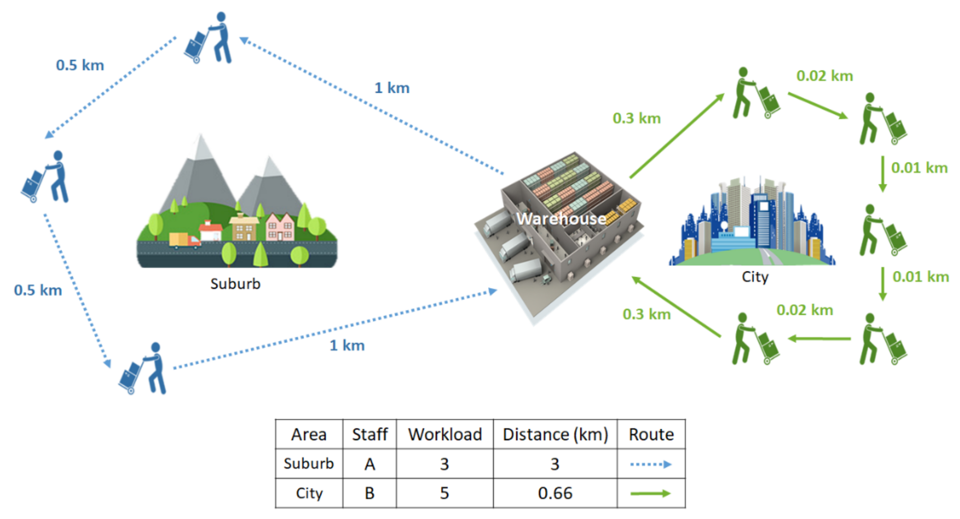
A performance bonus is usually calculated using piece rates or commissions based on freight charges. For example, an SD who delivers a package would receive a fixed amount as a performance bonus. Alternatively, an SD who picks up a package from a customer can earn a commission based on the charge for the package. However, these calculation methods may not be fair to all SDs. Typically, a region serviced by a logistics company is divided into numerous subregions, with each SD responsible for one subregion. Furthermore, the characteristics of each subregion may be different, as presented in Figure 1. If an SD is responsible for a subregion in which the order distribution is extremely dense, such as a district of a city, the SD can complete numerous orders in a short time. By contrast, the order distribution may be less dense in other areas, such as suburbs and remote districts, where customers are often far from each other and an SD responsible for such an area will therefore complete fewer orders; however, this does not mean that they are not working as hard as other SDs in areas with dense order distribution. The model developed in this study not only incorporates performance bonuses into the VRPTW but also alters the calculation method for identifying the load balance among SDs. This makes the calculation of performance bonuses fairer for all SDs.

The proposed model accounts for the performance bonus balance issue. However, in practical applications, the time required to solve this model using existing optimization software is too long to ensure a timely response. Therefore, we proposed an algorithm that incorporates an agent bidding mechanism and a nearest urgent candidate (NUC) heuristic. The algorithm was implemented and tested using a set of problem instances, and the obtained solutions were found to balance the performance bonuses of SDs and simultaneously plan favorable routes.

The remainder of this paper is organized as follows: Section 2 presents a review of the relevant literature. Section 3 explains the mathematical model of the problem. Section 4 describes the procedures of the proposed NCU algorithm in detail and Section 5 discusses the performance of the proposed NCU algorithm. Finally, Section 6 presents conclusions and recommendations for future studies.

2. Related Work

Developments in e-commerce have led to changes in customer behavior, with services such as home delivery, in-store pickup, and parcel lockers now commonly being used. The demand for delivery services is increasing. In addition, increased urbanization has made urban traffic flow more complex. The transport of goods is thus now extremely complicated, and logistics companies face numerous transportation challenges.

The proposed model considers some practical constraints for solving the VRPs that are faced by logistics companies. The problem addressed herein can be traced back to the traveling salesman problem (TSP) [6]. The TSP entails the following question: if a salesman needs to visit numerous cities, where the locations of and distances between each city are known and each city must be visited once, after which the salesman returns to the first city, what is the distance traveled of the shortest route? The TSP is also a special instance of the VRP. It is an NP-hard problem and has been widely studied in the field of operations research [7].

To make the VRP more applicable to practical situations, previous studies have used various target types; for instance, minimizing the number of vehicles and/or transit time [8,9] or adding more constraints, such as soft time window considerations and various vehicle load limits [10,11]. The classification of the characteristics of a VRP is described below.

VRPs are often characterized by divisions into vehicles, stations, demand, operating types, and cost structures [12]. However, human-related factors were discussed less frequently in the relevant research. Studies have not discussed operator performance bonuses within VRPs. Thus, the present study included the constraint of performance bonus balance in the mathematical model to understand its effect on this type of problem.

In this section, we discuss some relevant studies that were used as references to develop the mathematical model and design the algorithm in this study. In some studies, the VRP was altered; for example, the objectives were changed, restricted calculations were performed, or the establishment of stations and vehicles with certain operation modes was considered.

Chen, et al. [9] used the minimum number of vehicles and shortest travel distance as the target of a dual-objective mathematical model. Then, they incorporated vehicle capacity and time windows as constraints in the model. Additionally, they proposed a variable neighborhood search algorithm with compound neighborhood operators to explore a wider search area and to solve the two objectives of the model simultaneously. By contrast, in the present study, an objective function that simultaneously considers the number of vehicles, overtime of the time window, number of operators, and travel time was constructed. To reduce the problem’s complexity, which is high because of its multiple objectives, all items are converted so that they all have the same cost unit. Subsequently, the objective function is converted into a target that aims to minimize cost.

Regarding the operation mode, Lalla-Ruiz, et al. [13] discussed the multidepot open vehicle routing problem (MDOVRP). In the MDOVRP, there are multiple depots and some constraints on how each vehicle operates. First, the vehicles are initially located at multiple stations. Second, once they deliver goods to the final customer on their route (i.e., when they complete their tasks), they are not required to return to the warehouse. Lalla-Ruiz et al. solved the MDOVRP by using a proposed mixed-integer programming formulation to minimize the total travel cost.

Other studies have solved VRPs using other methods. The present literature review revealed that heuristics or improved heuristics were also used for solving such problems, in addition to mathematical models. Some studies that used such methods are discussed below.

De Grancy and Reimann [14] solved the VRPTW with multiple service workers by considering the trade-off between reducing vehicle and driving costs and paying employees. They divided the process of obtaining a solution into two stages. In the first stage, self-proposed cluster-construction heuristics were used to partition customers according to location and time windows. In the second stage, routes were planned on the basis of the clustering results. Poonthalir, et al. [15] proposed a constraint-based heuristic to solve the VRPTW. This approach was also divided into two stages. First, every customer was assigned to a cluster on the basis of spatial constraints and a devised priority metric. Second, a route was planned according to urgency, which was determined according to time limits.

Numerous studies have thus used two-stage methods to solve VRPs. For example, Bodin, et al. [12] used the cluster-first, route-second method in which the demand points are divided into several groups, and this enables the optimal method for planning vehicle routes to be obtained. This greatly simplified the problem and thus reduced the solution time. The cluster-first, route-second method relies on excellent clustering; if the clustering is not good enough, the results of the groups are not favorable and may even prevent route planning in the second stage. Thus, in terms of path planning, we referred to the technique proposed by Poonthalir, et al. [15]. Through the NUC approach, we used urgency and distance as the basis for route planning.

Time windows are usually considered to be a type of demand constraint in VRPs. Time window constraints are not applied to VRPs alone but are also used in other areas. We next discuss recent related applications of time windows.

Kittilertpaisan and Pathumnakul [16] defined a VRPTW in the field of agricultural planning. Based on the general VRPTW model, they used a hard time window to determine the start time of a harvester and proposed a mathematical model to solve a mechanized sugarcane harvesting problem. Rincon-Garcia, et al. [17] considered time-dependent travel times in a VRP, wherein vehicle routing is affected by the degree of traffic congestion. Not accounting for traffic congestion may lead to underestimating travel times and missed deliveries. Therefore, they combined large and variable neighborhood search techniques to propose a hybrid metaheuristic algorithm that solves problems with hard time windows. Mao, et al. [18] also considered time-dependency in a VRP; however, the specific time-dependency was considered to be uncertain and the time windows were soft ones. They used a variation of the artificial bee colony algorithm to solve the mathematical model of transportation costs and expected total service costs.

In previous studies, either hard or soft time windows were used [1,19]:

Hard time windows: the demanded service must be performed within the customer-stipulated time interval.

Soft time windows: the demanded service can be performed outside of the customer-stipulated time interval; however, doing so will incur penalties.

In this study, soft time windows were incorporated into the VRPTW because this situation is closer to real life than hard time windows are [20]; the penalties can be adjusted to ensure a feasible solution. Therefore, we further discuss soft time windows below.

The soft time windows used in previous studies can be divided into different types according to the penalty calculation methods used. Generally, penalties are calculated for both early and late delivery outside of the agreed-upon time interval. However, in some models, a time interval is considered soft on only one side of the interval and is referred to as a semisoft time window. In this type, the soft side of the time window is usually considered the later side. Setak, et al. [21] proposed a mixed-integer linear programming formulation to discuss a variant supply chain network that simultaneously considers pickup and delivery using semisoft time windows. For soft time windows in this model, penalties were only incurred for late arrival and no penalty was incurred for early arrival.

One type of soft time window is more similar to a hard time window. Niknamfar and Niaki [22] used a window with a certain degree of flexibility. If a delivery is scheduled to occur outside of certain upper and lower boundaries, the penalties are equal to infinity and thus such a schedule is unacceptable. In the penalty cost function, $P_i$ is the penalty of node (or customer) $i$; $C_e$ and $C_l$ are the unit penalty costs for early and late arrival outside of the agreed-upon time interval, respectively; and $a_i$ is the arrival time at node $i$.

$$P_i=\left\{\begin{array}{c}\infty , \mathrm{if} a_i<L{E}_i\\ C_e\left(E_i-a_i\right), \mathrm{if} L{E}_i\le a_i<E_i\\ 0, \mathrm{if} E_i\le a_i\le L_i\\ C_l\left(a_i-L_i\right), \mathrm{if} L_i<a_i\le U{L}_i\\ \infty , \mathrm{if} U{L}_i<a_i\end{array}\right.$$

(1)

The agent-based model (ABM), also known as the multi-agent system, has recently been used in numerous fields. As a microscopic computational model, it is used to simulate and predict complex phenomena by simulating the actions and interactions of multiple autonomous agents (e.g., organizations and teams).

Mes, et al. [23] used an ABM to solve the real-time scheduling problem of full truckload transportation orders with time windows. Two types of agents were included: intelligent vehicle agents and job agents. The former communicates with the latter about how to minimize transportation costs and schedule routes. This method yields a more stable level of service and makes schedule adjustments more convenient. Lim, et al. [24] proposed an iterative agent-bidding mechanism to optimize process planning. To reflect the market environment, this method was based on the dynamic integration of process and production scheduling. The currency value of each operation is adjusted in each iteration, and the resource agent rebids on these operations according to their currency value until the total production cost is minimized. In the present study, we referred to this iterative agent bidding mechanism in our algorithm. On the basis of the performance bonus, we designed agents to coordinate operations, identify appropriate routes, balance the bonuses given to all staff members, and minimize the cost.

In this study, we proposed a VRPTW with the consideration of a human-related factor, namely, performance bonus balancing. In addition, to solve the problem more efficiently, we also present a two-part heuristic algorithm by integrating an iterative agent bidding mechanism approach with the NUC heuristic.

3. Mathematical Model

The vehicle routing problem addressed in this study is based on the case of home delivery companies with only one depot, a fixed number of sales drivers (SDs), and a fixed fleet size. We solved the VRPTW for a number of known daily customer orders to obtain optimal routes. In contrast to previous VRPTWs, we considered the fairness of SD performance bonuses and the soft time windows of customers.

We made some assumptions to address this problem’s complexity and define how the model can be used: (1) The home delivery company aims to minimize the total operating cost and to balance the performance bonuses of the SDs. Performance bonus is calculated using freight charges. With the same delivering time, SDs could complete more orders in a dense order distribution area, such as a district of a city. However, this does not mean that a suburban SD is not working as hard as other SDs in areas with a dense order distribution. The proposed model developed in this study not only incorporates performance bonuses into the VRPTW but also alters the calculation method for identifying the load balance among SDs. This makes the performance bonuses fairer for all SDs.

Furthermore, (2) the company has only one depot; (3) the number of SDs is given, (4) each SD operates one vehicle; therefore, the fleet size is also given; (5) all vehicles are identical and have equal capacity (i.e., vehicles are homogeneous); (6) the demand from all customers is known; (7) each customer can be serviced by only one SD; (8) all customer time windows are soft; and (9) the demand from all customers is for pickup (or delivery). The notation used in the model is shown below.

In our mathematical model, the objective function, presented in Equation (2), minimizes the weighted sum of the performance bonus variations and the total travel cost. The model constraints are given by Equations (3)–(17). Equations (3) and (4) are the flow balance constraints that indicate that the flow at each node must be conserved. Equation (5) means that each SD must serve at least one customer. Equation (6) lets every node be served by only one SD. Equations (7) and (8) state that each SD must start from and return to the warehouse. Equation (9) limits the capacity of the vehicles used. Regarding the time window constraints, the waiting time and overtime of every node are stipulated in Equations (10) and (11), respectively, and the arrival time of the next node is calculated using Equation (12). Equation (13) indicates that the performance bonus of each SD must meet the minimum performance bonus. Equation (14) defines the performance bonus of every customer j, whereas Equation (15) calculates the performance bonus awarded for the return to the warehouse of each SD. Equation (16) calculates the total performance bonus awarded to each SD k. Finally, Equation (17) calculates the average of all SD performance bonuses.

$$min Z=\alpha {{\displaystyle \sum }}_{k=1}^v|b^k-b^{\mu }|+\beta \left({{\displaystyle \sum }}_{i=0}^n{{\displaystyle \sum }}_{j=0}^n{{\displaystyle \sum }}_{k=1}^v{t}_{ij}\times x_{ij}^k\times \gamma \right)$$

(2)

subject to

$${{\displaystyle \sum }}_{i=0}^n{x}_{ij}^k=y_j^k \forall k=1,\dots ,v, \forall j=1,\dots ,n+1 \mathrm{and} i\ne j$$

(3)

$${{\displaystyle \sum }}_{j=1}^{n+1}{x}_{ij}^k=y_i^k \forall k=1,\dots ,v, \forall i=0,\dots ,n \mathrm{and} i\ne j$$

(4)

$$x_{ij}^k=0 \forall k=1,\dots ,v, i=0, j=n+1$$

(5)

$${{\displaystyle \sum }}_{k=1}^v{y}_i^k=1 \forall i=1,\dots ,n$$

(6)

$${{\displaystyle \sum }}_{k=1}^v{y}_0^k=v$$

(7)

$${{\displaystyle \sum }}_{k=1}^v{y}_{n+1}^k=v$$

(8)

$${{\displaystyle \sum }}_{i=0}^n{y}_i^k\times q_i\le Q \forall k=1,\dots ,v$$

(9)

$$w_i=max\left\{e_i-a_i,0\right\} \forall i=0,1,\dots ,n$$

(10)

$$o_i=max\left\{a_i-l_i,0\right\} \forall i=0,1,\dots ,n$$

(11)

$${{\displaystyle \sum }}_{k=1}^v{x}_{ij}^k\times (a_i+w_i+o_i+s_i+t_{ij})={{\displaystyle \sum }}_{k=1}^v{x}_{ij}^k\times a_j \forall i,j=0,1,\dots ,n \mathrm{and} i\ne j$$

(12)

$$b^k\ge b_{min} \forall k=1,\dots ,v$$

(13)

$$b_j=q_j\times c+d\times {{\displaystyle \sum }}_{i=0}^n\left(t_{ij}\times {{\displaystyle \sum }}_{k=1}^v{x}_{ij}^k\right) \forall j=0,1,\dots ,n$$

(14)

$$b_M^k=d\times {{\displaystyle \sum }}_{i=0}^n\left(t_{ij}\times {{\displaystyle \sum }}_{k=1}^v{x}_{ij}^k\right) j=n+1$$

(15)

$$b^k={{\displaystyle \sum }}_{i=0}^n{y}_i^k\times b_i+b_M^k \forall k=1,\dots ,v$$

(16)

$$b^{\mu }=\frac{{{\displaystyle \sum }}_{k=1}^v{b}^k}{v}$$

(17)

Because the objective function includes an absolute value function and the constraints include the maximum value function, the model is nonlinear and cannot be solved easily. In this study, nonlinear functions are linearized according to the method reported in the literature, which facilitates solving the problem using optimization software.

The calculation of the waiting time and overtime of every node, given in Equations (10) and (11), was converted into the following:

$$w_i\ge e_i-a_i \forall i=0,1,\dots ,n$$

(18)

$$w_i\ge 0 \forall i=0,1,\dots ,n$$

(19)

$$o_i\ge a_i-l_i \forall i=0,1,\dots ,n$$

(20)

$$o_i\ge 0 \forall i=0,1,\dots ,n$$

(21)

To linearize the objective function, we rewrote Equation (2) as Equation (22) and added Equations (23) and (24):

$$min Z=\alpha \left(b^{+}-b^{-}\right)+\beta \left({{\displaystyle \sum }}_{i=0}^n{{\displaystyle \sum }}_{j=0}^n{{\displaystyle \sum }}_{k=1}^v{t}_{ij}\times x_{ij}^k\times \gamma +{{\displaystyle \sum }}_{i=0}^n{b}_i+{{\displaystyle \sum }}_{i=0}^n{o}_i\times \theta \right)$$

(22)

$$b^{+}-b^{-}={{\displaystyle \sum }}_{k=1}^v(b^k-b^{\mu })$$

(23)

$$b^{+},-b^{-}\ge 0$$

(24)

With these substitutions, Equations (10), (11) and (17) were converted into linear constraints. The linearized mathematical model is expressed as follows:

$$min Z=\alpha \left(b^{+}-b^{-}\right)+\beta \left({{\displaystyle \sum }}_{i=0}^n{{\displaystyle \sum }}_{j=0}^n{{\displaystyle \sum }}_{k=1}^v{t}_{ij}\times x_{ij}^k\times \gamma \right)$$

(25)

subject to

$${{\displaystyle \sum }}_{i=0}^n{x}_{ij}^k=y_j^k \forall k=1,\dots ,v, \forall j=1,\dots ,n+1 \mathrm{and} i\ne j$$

(26)

$${{\displaystyle \sum }}_{j=1}^{n+1}{x}_{ij}^k=y_i^k \forall k=1,\dots ,v, \forall i=0,\dots ,n \mathrm{and} i\ne j$$

(27)

$$x_{ij}^k=0 \forall k=1,\dots ,v, i=0, j=n+1$$

(28)

$${{\displaystyle \sum }}_{k=1}^v{y}_i^k=1 \forall i=1,\dots ,n$$

(29)

$${{\displaystyle \sum }}_{k=1}^v{y}_0^k=v$$

(30)

$${{\displaystyle \sum }}_{k=1}^v{y}_{n+1}^k=v$$

(31)

$${{\displaystyle \sum }}_{i=0}^n{y}_i^k\times q_i\le Q \forall k=1,\dots ,v$$

(32)

$$w_i\ge e_i-a_i \forall i=0,1,\dots ,n$$

(33)

$$w_i\ge 0 \forall i=0,1,\dots ,n$$

(34)

$$o_i\ge a_i-l_i \forall i=0,1,\dots ,n$$

(35)

$$o_i\ge 0 \forall i=0,1,\dots ,n$$

(36)

$${{\displaystyle \sum }}_{k=1}^v{x}_{ij}^k\times (a_i+w_i+o_i+s_i+t_{ij})={{\displaystyle \sum }}_{k=1}^v{x}_{ij}^k\times a_j \forall i,j=0,1,\dots ,n \mathrm{and} i\ne j$$

(37)

$$b^k\ge b_{min} \forall k=1,\dots ,v$$

(38)

$$b_j=q_j\times c+d\times {{\displaystyle \sum }}_{i=0}^n\left(t_{ij}\times {{\displaystyle \sum }}_{k=1}^v{x}_{ij}^k\right) \forall j=0,1,\dots ,n$$

(39)

$$b_M^k=d\times {{\displaystyle \sum }}_{i=0}^n\left(t_{ij}\times {{\displaystyle \sum }}_{k=1}^v{x}_{ij}^k\right) j=n+1$$

(40)

$$b^k={{\displaystyle \sum }}_{i=0}^n{y}_i^k\times b_i+b_M^k \forall k=1,\dots ,v$$

(41)

$$b^{\mu }=\frac{{{\displaystyle \sum }}_{k=1}^v{b}^k}{v}$$

(42)

$$b^{+}-b^{-}={{\displaystyle \sum }}_{k=1}^v(b^k-b^{\mu })$$

(43)

$$b^{+},-b^{-}\ge 0$$

(44)

4. Proposed Heuristic Algorithm

In this study, we proposed using a heuristic algorithm to solve this problem because the VRPTW is NP-hard. The proposed algorithm was divided into two parts. In the first part, an iterative agent bidding mechanism was used instead of Equation (23); in the second part, we used the NUC to plan routes. The algorithm aims to balance the performance bonuses awarded to SDs and, simultaneously, to identify favorable delivery routes.

Specifically, we introduce a multi-agent system into the algorithm and divide the program into several parts according to their functions (as shown in Figure 2). The proposed iterative agent bidding mechanism incorporates six types of agents: logistics, customer, bidding, order sequencing, scheduling, and data agents.

First, all parameters must be initialized and some data, such as transportation and labor costs, must be input into the algorithm. Furthermore, in the route planning system, every SD is modeled as a logistics agent and each demand node is a customer agent.

The logistics agents are responsible for storing information about SDs and importing it into the system; this information includes the vehicle capacity and performance bonus data. Customer agents have similar functions for customers; they import information such as customer coordinates, time windows, and service times into the system. The data agent calculates the distances depending on the departure and destination points and inputs them into the distance matrix. After the basic parameters have been set and the data agent has performed the data preprocessing, the core part of the algorithm is initiated.

The system next performs advanced route planning. This consists of two parts: route planning and the iterative agent bidding mechanism.

For route planning, we used the NUC to identify favorable vehicle routes. As described previously, after the bidding agent selects a logistics agent, the order sequencing agent uses the NUC to calculate the degree of closeness to the customer for each customer agent and uses the closeness to rank these customer agents.

The NUC is derived from the nearest neighbor heuristic, which is one of the most powerful heuristics used for route planning. It obtains an effective initial solution by assigning the closest unrouted customer to the SD and continues by assigning the next closest unrouted customer until all customers are assigned to an SD’s route or all constraints are met. If some constraints are infeasible, it cannot assign any customers to an SD’s route. In this case, it assigns customers to the next SD for a new route and repeats the process until all customers are served by an SD.

In the nearest neighbor heuristic, “closeness” only considers the direct distance. However, in the VRPTW, this method results in a violation of time window constraints. The proposed nearest urgent neighbor (NUN) heuristic, “closeness” considers two factors: direct distance ($d_{ij}$) and remaining time ($t_{ij}$). Closeness $=\alpha d_{ij}+\beta t_{ij}$, where $\alpha +\beta =1, \alpha \ge 0, \beta \ge 0$. To consider all possible customers and combinations, the NUN approach may take time to find the next closest unrouted customer. In this study, we thus used the NUC as the order-sequencing agent; it combines the NUN with a strategy in which some unrouted customer agents are excluded because the shipments exceed the vehicle’s capacity. This means that the “closeness” of a customer agent simultaneously considers the direct distance and remaining time. In addition, this strategy prevents the order-sequencing agent from sequencing the routes with the distance and time window of some customer agents. This enables the NUC to more quickly find a feasible route.

The bonus-based iterative agent bidding mechanism is proposed to solve the problem addressed in this study. Figure 3 shows the flowchart of the proposed algorithm; the notations for the same are shown below.

In this mechanism, no data are supplied by the data agent regarding each logistics agent’s performance bonus in the first iteration; thus, every logistics agent has an equal ability to select customer agents and win the auction. Assume that there are two logistics agents: 1 and 2. They are each given the same priority in step 1 and preliminary bidding rates are assigned to them. Equation (45) then describes the bidding rate of each agent, where $n$ is the number of logistics agents. Therefore, $n=2$ is obtained.

$$x_l^1=\frac{100}{n}\% \forall l=1,\dots ,$$

(45)

Regarding the priority setting, the bidding agent randomly selects a logistics agent. In step 2 (Figure 3), the bidding agent selects logistics agent 2 in the first round. With the NUC, the order sequencing agent calculates the “closeness”: $c_j^k$ of customer agent $j$ in step 3. The order sequencing agent uses the closeness to rank these customer agents. In this step, the “closeness” is based on the distance matrix ($d_j^k$) and remaining time ($r_j^k$) that are provided by the data agent and depend on the logistics agent $l$ that was selected in step 2. Then, in step 4, the scheduling agent chooses the customer agent with the best closeness and adds to the path of logistics agent 2.

After the first round, steps 2–4 are repeated until all customer agents are served by a logistics agent. The process of completing steps 2–4 indicates the completion of a round. In Figure 3, there are six customer agents; thus, there are six rounds and $k=6$. The completion of all six rounds concludes one iteration.

After the first iteration, each logistics agent’s performance bonus can be calculated: $t{p}_1^1$ and $t{p}_2^1$ in step 5. The value of $t{p}_l^i$ is the sum of the performance bonuses for customer agents that are selected in every round $k$ by each logistics agent $l$: $p_j^k$. Thus, in step 6, these are converted into the bidding rate for the second iteration using the following conversion equations:

$$t{p}_l^i={\displaystyle \sum }_{jϵC_{li}}{p}_j^k \forall i=1,\dots ,I \mathrm{and} \forall l=1,\dots ,L$$

(46)

$$M_{tp}^i={\displaystyle \prod }_{l=1}^{L}t{p}_l^i \forall i=1,\dots ,I$$

(47)

$$SU{M}_{tp}^i={\displaystyle \sum }_{l=1}^L\frac{{{\displaystyle \prod }}_{l=1}^{L}t{p}_l^i}{t{p}_l^i} \forall i=1,\dots ,I$$

(48)

$$x_l^{i+1}=\frac{M_{tp}^i}{t{p}_l^i\times SU{M}_{tp}^i} \forall i=1,\dots ,I \mathrm{and} \forall l=1,\dots ,L$$

(49)

First, all values in Equation (46) are multiplied. Then, the value is divided by its respective value. From this, a set of proportions is obtained, as summarized in Equation (48), that is equal to the value of each proportion divided by the total of these proportions. Finally, the results in terms of percentages are obtained:$x_1^{i+1}$ and $x_2^{i+1}$ in Equation (49). Steps 2–6 in this process are then repeated until the iteration is complete or satisfies the termination condition (i.e., all capacities of logistics agents are met). After the process is repeated, the fitness is calculated and the data agent outputs the result to the system.

5. Computational Results

In this section, we provide the results of the model and algorithm analysis and its relevant parameters, with the analysis divided into the following subsections. First, the effect of adding a performance bonus balancing constraint to the model was analyzed. Next, we used a small sample to compare the accuracy of the algorithm’s solution. Then, we analyzed the parameter combination used in the proposed algorithm. Finally, we solved large-scale problems using the parameter combination that was found to be most effective in the sensitivity analysis.

In this section, we considered the inclusion of a performance bonus in the formulated mathematical model. The C++ Gurobi library was used to solve our model. However, because our model is nonlinear, it must first be linearized, as described in Section 3. The detailed steps can be found in the previous section.

Two model types were used: unbalanced and balanced performance bonus models. In the unbalanced model, we removed the constraints on the performance bonuses described in Equations (23)–(25). Then, we used some simple examples to assess the increase in cost caused by adding the balancing constraint to the proposed model. We selected 20 nodes from Solomon’s VRPTW benchmark problems for use as simple examples. These 20 nodes were assigned to five SDs. We used two sets of data, C101 and C102, which have identical coordinate, demand, and service time data. The time window settings differed between the two data sets. In C101, every customer’s time window had a clear start time and end time, whereas there were no start times for some customers in C102; thus, these start times were set to 0 or $-\infty$. This also indicated that there was no additional waiting time in our model when these customers were serviced in advance.

Table 1. Computational results for costs.

Date Type	C101		C102
	Unbalanced	Balanced	Unbalanced	Balanced
Transportation cost	283.732	304.033	269.830	290.077
Performance bonus cost	683.732	704.033	669.830	690.077
Total cost	967.463	1008.067	939.660	980.153

and

Table 2. Computational results for performance bonuses.

Date Type	C101		C102
	Unbalanced	Balanced	Unbalanced	Balanced
Max performance bonus	155.0735	153.2116	177.3575	155.0735
Min performance bonus	121.1664	128.4440	103.0397	129.5139
Proportion = (max/min)	1.280	1.193	1.721	1.197

display the computational results for the two models.

Table 1 presents the data demonstrating that the cost incurred when using the unbalanced model was lower than that incurred when using the balanced model, but the cost difference between them was not large. Table 2 presents the performance bonus results. Adding the bonus constraints balanced the performance bonuses awarded to employees to a certain degree. The difference was particularly evident for C102: the ratio of the maximum to the minimum bonus was 1.721 for the unbalanced model.

In our proposed method, we included two parameter settings of the closeness for sequencing: the distance (α) and the remaining time (β) in the NUC.

In the sensitivity analysis, we used two parameter settings: α = D and β = T. The analysis was divided into ten combinations of parameters; for example, D1T9 indicates that the ratio of the distance is 0.1 and the ratio of the remaining time is 0.9. Figure 4 and Figure 5 exhibit detailed comparisons.

Figure 4 illustrates that the total cost increased with the distance. Further, the minimum cost was obtained for the parameter combination D2T8. Therefore, for closeness, we chose D2T8 as the parameter combination to test large-scale problems. By contrast, Figure 5 shows that irrespective of the parameter combination, the α and β values did not affect the performance bonus balance of results. In summary, on the basis of the sensitivity analysis depicted in Figure 4 and Figure 5, we chose D2T8 as the parameter setting for large-scale problems.

For both C101 and C102, the cost of the unbalanced model was slightly higher than that of the balanced model (as shown in Figure 6). However, the proportions we obtained using the two models were substantially different for C102: 1.721 and 1.197 for the unbalanced and balanced models, respectively. Despite the increased costs, the balanced model achieved a balanced performance bonus distribution.

The results presented in the previous section indicate that the model that used balancing constraints did indeed balance the performance bonuses awarded. However, this model required too much time to obtain a solution in practice. Thus, the proposed algorithm was used to effectively reduce the computing time while simultaneously maintaining the solution quality. For this reason, we used three types of small-scale problems in this section. The data were obtained from Solomon’s VRPTW benchmark problems. As an example, the data entry “20pv2” indicates that 20 nodes were assigned to two SDs, whereas “20pv5” indicates that 20 nodes were assigned to five SDs.

Table 3. Computational results for small-scale problems.

Date Type	Mathematical Model			Proposed Model
	20pv2	20pv5	30pv3	20pv2	20pv5	30pv3
Total cost	992	1008	1012	673	1228	932
Transportation cost	265	304	246	157	396	206
performance bonus cost	625	704	766	517	796	726
Overtime cost	101	0	0	0	35	0
Max performance bonus	327.09	153.21	285.88	297.23	172.26	285.88
Min performance bonus	298.23	128.44	238.29	219.49	133.06	219.49
Proportion = (max/min)	1.10	1.19	1.20	1.35	1.29	1.30
Time (s)	276,484	226,195	446,428	450	1122	1019

presents the computational results.

The differences between the costs obtained using the model and the proposed method were insubstantial, and all performance bonus proportions were within the range of 1.2–1.4. However, the difference in computational time was considerable: the smallest difference obtained was a factor of 200.

After testing the simple examples, we used four of Solomon’s VRPTW benchmark problems again for our large-scale problems: C101–104. As stated previously, some customers in C102 had time windows with no start times. The data in C103 and C104 were identical, except that the proportions of customers who had not stipulated start times differed. Customers in C102–104 accounted for 25%, 50%, and 75% respectively.

Figure 7 illustrates the convergence of the proposed method—an obvious convergence was obtained before 400 iterations. When the number of customers who did not stipulate a start time was increased, the convergence speed also increased. This may have been because an increased number of customers without a start time relaxed the constraints on the time windows, thereby simplifying the problem-solving process.

Because the mathematical model took too long to find a solution, we used Gurobi calculations for 8 h solutions to compare the total costs and bonus proportions (Figure 8). The results for the large-scale problems (

Table 4. Computational results for large-scale problems.

Date Type	Total Cost (USD)		Proportion
	Proposed Method	Mathematical Model	Proposed Method	Mathematical Model
C101	10,195	62,864.071	1.686	1.200
C102	8045	57,523.945	1.678	1.20
C103	7427	30,248.337	1.532	1.20
C104	5147	14,873.891	1.496	1.20

) indicated that the total computational cost when C104 data were used was lower than when other data types were used. The bonus proportions that were calculated using the mathematical model were substantially lower than those obtained using our proposed method. This was because the performance bonus balance was constrained to be less than 1.2 in the mathematical model; otherwise, the solution would be deemed infeasible.

6. Conclusions

In this study, we considered performance bonuses within VRPTWs, which have never been discussed previously in the related literature. In most logistics companies, performance bonuses are usually awarded to maintain efficiency and balance the workload. However, practical considerations mean that the performance calculation method is not fair to all staff. Therefore, this study altered the method used to calculate bonuses to ensure that the awarded performance bonuses were more balanced. Further, to shorten the operation time, this study presented an algorithm that consisted of an iterative agent-bidding mechanism and NUC. The results demonstrated that adding the performance bonus constraint to our model balanced the performance bonuses to a certain degree. By contrast, the sensitivity analysis demonstrated that α and β values did not affect the performance bonus balance of results.

In this study, we considered the balance of performance bonuses and developed algorithms to speed up the solving times. However, we only considered the problem in a static situation. In reality, it is often necessary to consider dynamic factors. For example, travel time is affected by traffic flow. In addition, some customer demands must receive an immediate response; however, the problem of rush orders was not addressed in this study.

For future research, the research could include current traffic flow factors in operations when computing travel time and consider necessary changes to routes over the course of a workday. Furthermore, recent hot topics in this field relate to the application of VRPTW in the transportation of elderly or handicapped people and VRPTW for home health care (HHC) [25]. To increase the practicality of the method, we intend to build a rush order structure into the algorithm or use other heuristic approaches.