Article

Built Environment Typologies Prone to Risk: A Cluster Analysis of Open Spaces in Italian Cities

by
Alessandro D’Amico
1,2,
Martina Russo
1,*,
Marco Angelosanti
1,
Gabriele Bernardini
2,
Donatella Vicari
3,
Enrico Quagliarini
2 and
Edoardo Currà
1
1
Department of Civil, Building and Environmental Engineering, Sapienza Università di Roma, 00184 Rome, Italy
2
Department of Construction, Civil Engineering and Architecture (DICEA), Università Politecnica delle Marche, 60121 Ancona, Italy
3
Department of Statistical Sciences, Sapienza University of Rome, 00185 Rome, Italy
*
Author to whom correspondence should be addressed.
Sustainability 2021, 13(16), 9457; https://doi.org/10.3390/su13169457
Submission received: 8 June 2021 / Revised: 9 August 2021 / Accepted: 11 August 2021 / Published: 23 August 2021
(This article belongs to the Section Hazards and Sustainability)

Abstract

:
Planning for preparedness, in terms of multi-hazard disasters, involves testing the relevant abilities to mitigate damage and build resilience, through the assessment of deterministic disaster scenarios. Among risk-prone assets, open spaces (OSs) play a significant role in the characterization of the built environment (BE) and represent the relevant urban portion on which to develop multi-risk scenarios. The aim of this paper is to elaborate ideal scenarios—namely, Built Environment Typologies (BETs)—for simulation-based risk assessment actions, considering the safety and resilience of BEs in emergency conditions. The investigation is conducted through the GIS data collection of the common characteristics of OSs (i.e., squares), identified through five parameters considered significant in the scientific literature. These data were processed through a non-hierarchical cluster analysis. The results of the cluster analysis identified five groups of OSs, characterized by specific morphological, functional, and physical characteristics. Combining the outcomes of the cluster analysis with a critical analysis, nine final BETs were identified. The resulting BETs were linked to characteristic risk combinations, according to the analysed parameters. Thus, the multi-risk scenarios identified through the statistical analysis lay the basis for future risk assessments of BEs, based on the peculiar characteristics of Italian towns.

1. Introduction

Disasters caused by natural hazards can trigger chains of multiple disastrous events over different spatial and temporal scales. Multi-hazard and multi-risk assessments consider interactions between different risks, evaluating triggered events, cascade effects, and the rapid increase of vulnerability during successive hazards [1]. As many regions of the world become subject to multiple hazards [2], the number of people affected by them keeps increasing. According to the report of the World Bank on the main hotspots of natural hazards [3], about 3.8 million km2 and 790 million people in the world are relatively highly exposed to at least two hazards, while about 0.5 million km2 and 105 million people are exposed to three or more hazards. Climate change is likely to further increase the exposure to multiple risks, affecting the magnitude, frequency, and spatial distribution of hazardous and disastrous events [4]. The overlap of different risks refers to both sudden-onset disasters (SUOD) (e.g., earthquakes, hurricanes, floods) and slow-onset disasters (SLOD) (e.g., drought, pollution, heatwaves, epidemic diseases) [5,6,7].
As Kappes et al. stated in their review on multi-hazard risks, there is a clear need to examine the frameworks employed in the field of risk management, along with the interactions between science and practice in terms of knowledge transfer and applicability of results [8]. The challenges for the development of multi-hazard approaches are related not only to the applicability of the results, but also to the link between risk assessment and decision making. These joint topics are essential for the development of an appropriate mechanism by which to communicate and transfer knowledge about the risks to various stakeholders [9]. This is especially the case when considering the built environment (BE) as a structured network of physical elements (e.g., open spaces, the facing built elements, and the other artifacts included into them) and when hosting users exposed to different risks [10,11,12]. Nevertheless, there remain barriers to the application of multi-risk assessments in the BE.

1.1. Built Environment and Multi-Risk Approach

As highlighted by Arosio, Martina, and Figueiredo, the approach to risk assessment needs to be holistic, as “the whole is more than the sum of its parts” [13]. It calls for an expansion of the current quantitative risk assessment paradigm, as well as measures to frame the study of interlinked disasters. Several different approaches have been developed in this research field, including the multilayer single hazard approach, in which the hazard potential or risk from one particular physical phenomenon is considered in isolation. This approach is one of the most common; however, it has shown limitations in considering interactions [14]. Other approaches are based on standardization schemes, combining distinct hazards through the use of indices and semi-quantitative approaches [8]; still others use economic metrics such as monetary loss. Monte Carlo simulations represent the dynamic evolution of risk and, hence, introduce the potential for evaluating extreme loss events [15]. Approaches based on the simulation of evacuation behaviours can relate users to risk assessment and the definition of risk mitigation strategies in BEs [16].
A key question is related to the continued growth of losses from natural disasters, considering the increasing scientific knowledge on multi-risk approaches [2,17]. One reason is the increasing value of assets exposed to hazards. Planning for preparedness for multi-hazard disasters can test capabilities to mitigate damages and build resilience to disasters, through the use of deterministic disaster scenarios. Even though such approaches are often practical and useful, a limited number of scenarios cannot test the full spectrum of possibilities of impacts and interactions [18]. To summarize, a multi-risk analysis is a complex problem involving a variety of challenges. One of the most significant elements to be considered is risk-prone assets [19], which represent the fundamental part of the elaboration of risk scenarios. As defined by Schmidt et al. [19], “elements at risk or assets are spatio-temporal phenomena, valued by human society, and under threat to be damaged by hazards (i.e., buildings, streets, lifelines, people)”. These assets are defined by their location and spatial extent, as well as by their exposure and vulnerability to specific hazards [19].
Among risk-prone assets, open spaces (OSs) have a significant role in the characterization of the BE and represent a decisive factor for risk assessment [12,20]. OSs are directly connected with the exposure of the inhabitants, building vulnerability, and site hazard level [21]. The classification of BEs depends on both the physical features of the BEs themselves and social aspects. In fact, while the flexibility, redundancy, and modularity of the BEs guarantee the organization of the strategic function, preparedness at the local level increases the ability to absorb shocks [10]. Therefore, the effect of disasters is affected by the presence of users combined with the features of the BEs, mainly referring to those placed in urban areas, which are characterized by complex issues, such as the overall layout of the urban fabric and user densities. The characteristics of OSs are common to national and European contexts, mainly those related to BEs in urban and historical areas, which are worth investigation as they are affected by risk-increasing exposure and vulnerability conditions. Thus, the OS in a BE is a representative urban portion from which to develop multi-risk scenarios.

1.2. Towards the Idealization of the Built Environment

Several methods have been investigated in the scientific literature to face the problem of multi-risk scenarios. Often, these studies have based their analysis on the same case studies, including their peculiarities. Some of them have tried to elaborate the classification of BEs, based on a specific risk [22] or regional surveys of OSs [23]. In their research, Mandolesi and Ferrero [23] have investigated all the OSs in the Piceno area of the Marche Region of Italy, defining recurring typologies of this type of BE.
Some recent studies have applied a similar methodology, working on the idealization of the BE. Among them, we surely have to cite Zuccaro et al. [24,25], who conducted a structural analysis on a territorial scale, and Morganti et al. [26,27], who considered energy investigation in urban fabrics. These are deductive approaches, which start from real case studies to idealize types. Zuccaro et al. [24,25] worked on the idealization of constructive typologies, analysing some common parameters derived from the observation of damage that had occurred during seismic events in the Italian territory. From this classification, based on expert judgment, some construction types are derived to elaborate on a structural analysis on a territorial scale. Morganti et al. [26,27] studied urban metrics related to solar performance, as derived from eight basic variables which are widely common in urban and building studies. Each metric gives information on some qualitative aspects of the urban form, such as the shape of the buildings, the plot patterns, or the street network, with the aim to idealize the urban fabric to be investigated. At the macro scale, similar research has been performed using fast surveys. Other examples oriented towards risk assessment and the application of simulation (mainly in SUODs such as floods) [16,28] have been proposed in previous works, based on the analysis and classification of real-world scenarios into typical conditions through the use of quick assessment methods (e.g., geometric-based). Finally, recurring indoor built environment scenarios have also been used in fire safety assessments, in order to test the capabilities of simulation models [29]. Such studies selected the case study format to elaborate the idealization of BEs in different ways, according to the relevant parameters considered.
Given this correlation between the idealization of the BE and the multi-risk perspective, such works have suggested that the parameters to be considered should be related both to the specificities of the BE to be assessed and the risks affecting it. In particular, the present work is part of an Italian PRIN (Projects of Relevant National Interest), entitled BE S2ECURe “(make) Built Environment Safer in Slow and Emergency Conditions through behavioUral assessed/designed Resilient solutions” (grant number: 2017LR75XK), supported by MIUR (the Italian Ministry of Education, University, and Research). The BE S2ECURE project is focused on some specific risks: for the SUODs (sudden-onset disasters), earthquakes and terrorist attacks; for SLODs (slow-onset disasters), heatwaves and pollution. Thus, the parameters considered in this work are related to these specific risks. Furthermore, this project focuses on the OSs, in view of their aforementioned importance for the resilience and safety of the BE, and, in particular, on areal spaces (i.e., squares), in the context of Italian cities.

1.3. Work Aims and Research Approach

In view of the above, the aim of this work is to define typical scenarios, referring to areal spaces (i.e., squares) as significant OSs in the BE [21], and considering the Italian context as a reference. The characterization of these scenarios represents a significant step from BEs to built environment typologies (BETs), where BETs represent the idealization of common features of Italian OSs in BEs. This step allows for describing the open spaces at risk under common and typical conditions for the SUODs and SLODs considered in the BE S2ECURe project, then recreating basic inputs for multi-risk assessment actions through simulation-based methodologies [16,30,31].
According to the previous phases of the BE S2ECURE project, nine parameters emerged as significant to describe the BEs—according to their morphological, functional, constructive, and physical features—and evaluable as relevant for the risk assessment [32]. Those analyses were elaborated on the expert judgment and a statistical analysis developed on a preliminary data set consisting of 133 squares of main Italian cities. Given the nine input parameters, the final number of combinations was about 768 BE possibilities. This large quantity would require a huge computational effort to detect models in the urban environment and, hence, to evaluate the performance of whole BEs under disasters. Deriving from an uncritical combination, this high number of BEs does not yet represent a feasible basis for the development of multi-risk scenarios.
Thus, in order to establish the more suitable definition of BETs, the analysis of a great data set of OSs needed to be investigated. Hence, geographic information system (GIS) technology was used. GIS represents a convenient digital system to collect and compare spatial and geographical data, and has increasingly been used in spatial decision support systems [33,34]. In the past few years, GIS has emerged as a powerful risk assessment tool, in particular to assess risks from natural hazards. The information retrieved by querying the GIS database can serve as input to risk assessment models. GIS can also be used to acquire large amounts of data which, in this case, are useful in defining common characteristics of OSs. Therefore, it was considered a tool that is appropriate to this type of analysis.
Furthermore, to manage and investigate this large amount of data, a cluster analysis appears to be a promising research tool. Standard clustering and classification methods can be divided into two broad categories: supervised and unsupervised methods. In the supervised classification, the analyst builds classes from training samples, which are later used to classify new cases. The selection of the training samples can be based on data collection or expert knowledge. Conversely, in the unsupervised classification case, no ground truth is available, such that, in an explorative setting, the analyst needs to build classes whose numbers are unknown. A cluster analysis includes methods of unsupervised classification, which have been widely used in similar research fields. For example, in the study of Paliaga et al. [35] a cluster analysis was used to build classes of catchments, in terms of anthropogenic disturbance, in order to detect a possible link with flooding frequency in a Mediterranean area. An unsupervised classification is particularly useful when data or prior knowledge about the area under study are not available, as was the case in the present study. As classes are not known, clustering offers great potential in the process of data mining, in terms of discovering concepts, possibly within a concept hierarchy. In the present study, a cluster analysis led to the classification of BETs, which will be used in future steps of the BE S2ECURE project, as the basis for risk scenario assessment through simulation-based methods.
In view of the above, the paper structure is organized as follows. Section 2 provides the methods for the parameters selection and characterization in real BEs according to large open-access databases and then traces how to organize BETs basing on cluster analysis techniques. Section 3 offers the cluster analysis results and then describes each of the assessed BETs and their representation. Finally, Section 4 discusses the characterizing risks for each BET in view of (multi) risk assessment purposes, and then traces the advances and limitations of this work.

2. Materials and Methods

The methodology is structured in four main sections, following the scheme in Figure 1. Section 2.1 presents the parameters selected to perform the cluster analysis of the OSs in Italian BEs, according to the previous outcomes of the BE S2ECURe research project. Section 2.2 describes the process applied to extract data from GIS databases and provides the mathematical definition of each parameter to build the final data set. Section 2.3 defines the cluster analysis methods used, as well as how the analysis was performed and evaluated as meaningful. Finally, Section 2.4 illustrates the process for defining BETs from the clusters identified, by introducing critical classes for each parameter that allow for the description of the physical features of BETs.

2.1. Open Space Parameters for BET Definition

Following the outcomes of the BE S2ECURe research project [32], the analysis for the definition of BETs started from the parameters described in Table 1.
The nine parameters describe relevant characteristics of OSs prone to SLODs and SUODs, considered in the context of the BE S2ECURe project.
As for the other OSs in the urban built environment [36], P1 can be initially used to describe the general plan configuration of the BE where people gather, act, and move, just before and during both SLODs [37] and SUODs [10,12,38]. P1 is combined with P2 to vertically shape the BE, and to P8 to give a complete overview of the main geometrical issues of the BE, and concerning its ground plan [10]. Furthermore, the combination of such data with P4 completes the connection of the BE into the urban fabric [10,39].
Concerning SLODs, P1 and P2 influence the possibility to have cool-shaded areas and wind funnel-related effects, which have impacts on heat alleviation and pollutant dilution [39,40,41]. In this sense, P2 also characterizes the urban canyon effects, where high built fronts decrease the risk of solar radiant exposure of the OS, but wind flow might be reduced. In addition, P4 concerns SLODs, as the permeability of the OS relates to the ventilation of the space. Finally, depending on P8, the presence of a constant slope represents an obstacle to good ventilation conditions and, thus, to pollutant transport and/or dilution [42].
Regarding SUODs, P1 affects the spatial complexity of the BE and, above all, the possible initial position of people in it (especially in the case of overcrowding conditions), the possibility to have safe distances from specific buildings or intended functions (e.g., in the case of a terrorist act), and the spatial relationship between the BE parts in the evacuation layout [12,38,43,44,45]. These elements become relevant when combined with P4, as also noticed in indoor SUODs (e.g., in case of a fire evacuation) [46] and other SUODs affecting the urban environment (e.g., in case of flooding evacuation) [16]. In fact, P4 describes the presence of possible accesses to/exits from the considered BE and, thus, the permeability of the OS, with respect to the surrounding urban fabric, as well as that of the evacuation paths in it. Furthermore, in the case of a seismic event, P2 represents a critical parameter for quick damage assessment based on façade overturning [47,48]. High built fronts increase the probability that seismic-induced debris can make the OS unavailable, especially in the case of narrowness of the OS, thus increasing overcrowding conditions during post-earthquake evacuation [49]. Finally, P8 also affects the evacuation process, as height differences in the OS (including stairs) can limit both the motion and speed of users while moving either upstairs or downstairs, as pointed out by consolidated approaches to the evacuation analysis [50].
P3 describes the presence of the built fronts in the OS perimeter. Regarding SLODs, the presence of built fronts (combined with their structural type and the related morphological issues) and/or open sides could increase or decrease the heat concentration, depending on the orientation of the BE’s sides and the position of the sun [37,40]. Concerning SUODs, built fronts could increase the probability of damage scenarios, in both terrorist acts (e.g., in case of an explosion) and seismic events, while a free side of an OS represents physical boundaries reducing the number of possible evacuation roads [48,49].
P5 relates to functional issues in BEs. Considering SUODs, the presence of special buildings attracting visitors (including tourists) could represent special targets for terrorist acts, increasing the exposure for people hosted in the BE [22]. Concerning SLODs, special buildings can increase the exposure, in terms of numbers and types of people with possible health fragilities and risky conditions of overcrowding [51].
P6 refers to constructive issues of the BE. Regarding SUODs, it affects the structural performance of the built fronts and the disaster-affected damage in the case of both seismic events and terrorist acts (e.g., explosions) [44,48]. Conversely, this parameter may have limited influence on SLODs, due to the typological surface materials related to the specific constructive types of the built elements [52,53]. Similarly, P7 relates to SUODs, as it represents significant structural weakness in the global behaviour of the built fronts. Meanwhile, concerning SLODs, P7 represents places with low levels of heat concentration (shaded space) and wind velocity (obstructed wind flow).
Finally, P9 enriches the spatial description of the OSs, which can affect the motion of people before and during an emergency scenario [10]. As far as SUODs, green areas may be used as a refuge or temporary shelter. In the case of a seismic event, people seem to be attracted by trees and street furniture during the shake, in order to gain stability [54]; in the case of a terrorist act, people can move toward a green area as a barrier against the source of the attack (e.g., explosion, shots) [44]. At the same time, green areas could represent obstacles to evacuation, depending on their positions in the OSs and their dimensions, as has also been reported in general studies on evacuation in the built environments [55]. Concerning SLODs, the green areas have a mitigating role in the increase of temperature and provide shaded areas [37,56,57]. Similarly, the green infrastructure increases the adsorption capabilities of air pollutants. The size and location of green areas can affect the impact on SLODs, for instance, large green elements may result in wind obstruction.
The nine parameters have been divided into fast and detailed categories, according to the principle of quick collecting methods to assess BE risk scenarios. Parameters for a fast analysis include data already available at a wide scale (i.e., GIS data), and suitable for accomplishing a fast statistical analysis; meanwhile, parameters in the detailed analysis category consist of data that need direct surveys to be collected.
  • Parameters for a fast analysis (morphological, geometric, and functional characteristics): P1, P2, P4, P5, P8, and P9;
  • Parameters for a detailed analysis (constructive characteristics): P3, P6, and P7.
As highlighted by Quagliarini et al. [22], sources of data that are easily available are preferred, in order to avoid costly in situ surveys, and permit the reproduction of the workflow by non-expert technicians. In this specific case, the detailed parameters are not secondary for the BE analysis, but need to be investigated through in situ surveys, as no reliable database for these data is available. Parameters for the detailed analysis are not included in the present study but could be further considered as additional attributes to deeply characterize the case studies.
Therefore, the analysis performed in this paper is based on five parameters for a fast analysis. As described in Table 1, the definitions of the parameters have been elaborated, according to the data which are extractable from GIS databases.

2.2. GIS Databases and Parameter Extraction

Among the many available databases, the authors selected two specific databases containing information related to the description of the BETs, according to the parameters identified for the analysis (Table 2).
OpenStreetMap (OSM) is a collaborative project to create an open-content license map of global geodata. The creation and growth of OSM have been motivated by restrictions on the use or availability of map data across much of the world, as well as the advent of inexpensive portable satellite navigation devices. Despite the growing amount of data in OSM, an additional official structured database—that of the Italian Ministry of Environment (MinAmb)—was necessary for this research.
GIS software is characterized by the possibility to interrogate a source of data in a spatial context, in order to obtain specific answers. These questions (called queries) are sets of commands and rules that are used to browse a database.
According to the ArcGIS dictionary [58], a query is a request that examines features or attributes to display those records that satisfy user-selected criteria. In the GIS environment, queries are divided into attribute queries and location/spatial queries. Attribute queries ask for information from tables associated with features or standalone tables associated with the GIS. Attributes can be numeric values, text strings, Boolean values, or dates. Location/spatial queries are derived directly from the positions of features on the map. In this way, in a GIS environment, the features related to the records selected by the process are highlighted on the map, as well as in the table of attributes.
All queries, both attribute and location/spatial ones, have three main parts: a source, a filter, and a relationship. The source can be a table or feature class. The filter can be an attribute value, or a shape or feature. The relationship between the source and the filter is based on specific operators, such as comparison operators (=, <>, >, >=, <=), logical operators (LIKE, AND, OR, and NOT), or spatial operators (Intersect, Are Within a Distance Of, Contain, Are Contained By…).
In the presented paper, spatial queries (performed using “Select by Location”) deal with vector data and use a shape as a filter and its relationship with features in the source layer. The choice of a spatial operator (i.e., the relationship by the query) depends on the types of features that are used for the source and filter.
GIS environments are also characterized by the opportunity to perform spatial analysis to pool spatial information (i.e., locations, attributes, and relationships of features) from many sources and obtain new and additional meanings from GIS data by applying a set of spatial operators. Inside GIS software, to put into practice the concept of spatial analysis, geoprocessing operations are used to manipulate GIS data. A geoprocessing operation takes an input data set, on which it performs an operation, and returns its result as an output data set. Common geoprocessing operations include geographic feature overlay, feature selection and analysis, topology processing, raster processing, and data conversion [58]. In this sense, geoprocessing employs appropriate processing tools to conduct spatial analyses.
In the present paper, in order to achieve a proper GIS implementation of the parameters described in Table 1, suitable queries and processing tools were chosen in the QGIS software, version 3.16 [59] (Table 3).
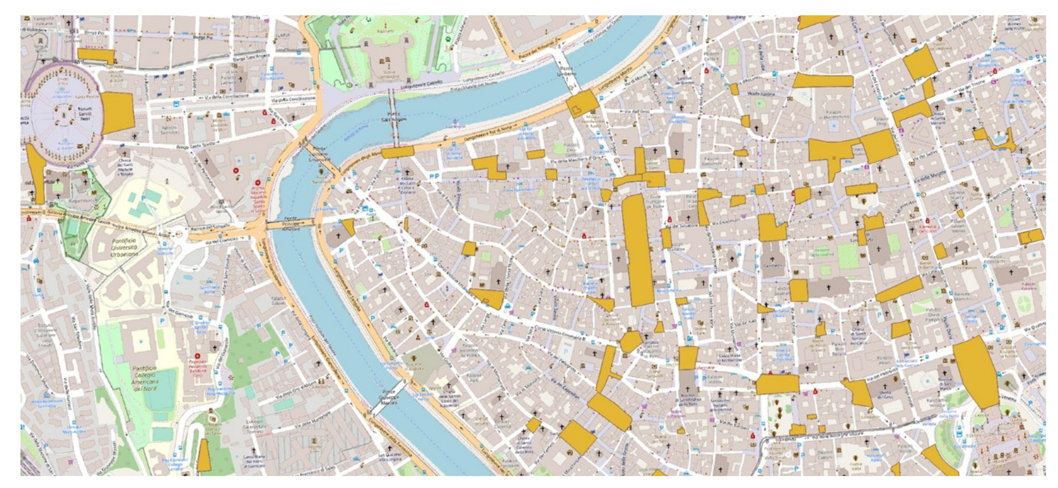
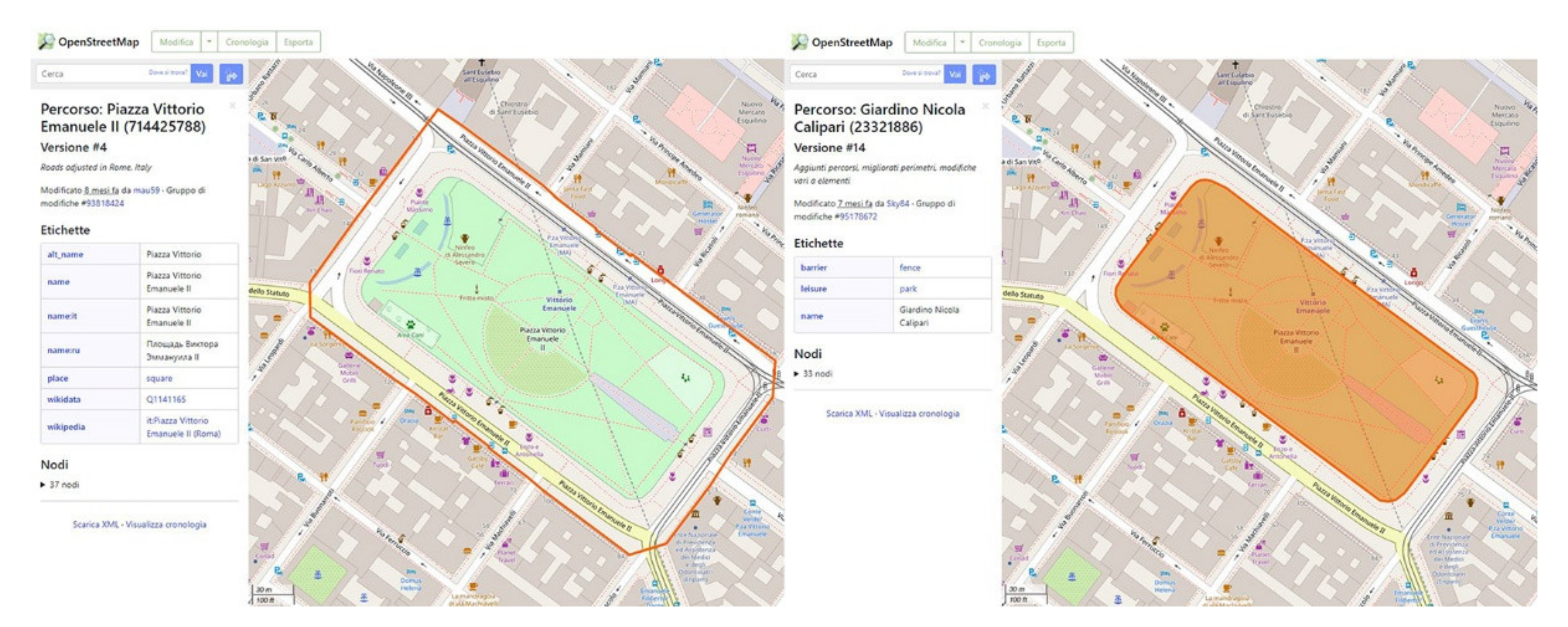
As for the queries, we focused on the OSM query place = square (Figure 2), which is used to map a town or village square, usually defined as a paved and open public space (generally of architectural significance) surrounded by buildings in a built-up area. According to its definition [60], the majority of locations satisfying tag place = square are paved and suitable for open markets, concerts, political rallies, and other events that require a solid surface. They are also known as city, urban, public, or market squares; therefore, they are usually named.
As for the processing tools (Table 3), in this research, we drew a distinction between data-extraction and data-fixing tools. In the first group, the following processing tools were chosen to extract new information from GIS databases:
  • Minimum oriented bounding box—to calculate the rotated rectangle of the minimum area that covers each OS, to extract its area (AMOBB);
  • Minimum circumscribed circumference—to calculate the minimum circumscribed circumference that covers each OS, to extract its diameter (d1) and radius (r1);
  • Inaccessibility pole—to find the centre of the maximum inscribed circumference for each OS, to extract its diameter (d2) and radius (r2);
  • Buffer—to create a buffer area for all elements in an input vector, using a fixed or dynamic distance.
In the second group, the following processing tools were used to fix data and for data correspondence between geometries from the GIS database:
  • Merge—to combine multiple vector layers having the same type of geometry into a single vector;
  • Intersection—to extract the parts of the overlapping elements in the input and overlap layers. The overlapping geometry attributes from both the input and overlay layers are assigned to the elements of the output intersection layer;
  • Fix geometry—to create a valid representation of a given invalid geometry without losing any of the starting vertices;
  • Join attributes by locations—to create a new vector with additional attributes added to the attribute table. The additional attributes and their values are taken from a second vector. A spatial criterion is applied to select the values from the second vector that are added to each element of the first vector and are part of the result.
Parameter 1 was elaborated as the product of the area regularity values and the radius ratio values (Equation (1)):
P 1 = P 1 a × P 1 b = A r e a   r e g u l a r i t y × R a d i u s   r a t i o .
The area regularity and radius ratio are defined as follows:
P 1 a = A r e a   r e g u l a r i t y = A A S   m 2 A M O B B   m 2 ,
where
  • AAS is the area of the considered OS, and
  • AMOBB is the area of the minimum oriented bounding box of the considered OS.
The oriented bounding box shows differences in approximation between regular shapes and irregular or composite ones. In this way, the higher the area regularity attribute, the more regular/quadrangular the shape of the OS.
The radius ratio (Equation (3)) was computed as a comparison between the minimum circumscribed circumference and the inaccessibility pole of the OSs:
P 1 b = R a d i u s   R a t i o = r 2   m r 1   m
where
  • r2 is the radius of the maximum inscribed circumference, calculated through the inaccessibility pole; and
  • r1 is the radius of the minimum circumscribed circumference.
On the one hand, the minimum circumscribed circumference processing tool algorithm calculates the minimum circumscribed circumference that covers each element in an input layer. On the other hand, the inaccessibility pole processing tool [61,62] is herein defined as the centre of the largest OS inscribed circle. It is the visual centre, the point within an OS that is the farthest from an edge. Contrary to the concept of centroid, if the shape is concave or has a hole, the inaccessibility pole will not fall outside of the shape. In the present paper, we use the inaccessibility pole processing tool, which uses the poly-label algorithm [61]. This tool is based on an iterative approach, which guarantees finding the true inaccessibility pole coupled with a specified tolerance (in layer units). More precise tolerances require more iterations and, as such, will take longer to compute. The radius of the maximum inscribed circumference, calculated as the distance from the pole to the edge of the polygon, will be stored as a new attribute in the output vector. In this sense, the concept of an inaccessibility pole differs substantially from the centroid concept, as it creates a new vector of points, where the points represent the centroid of the geometries of an input vector.
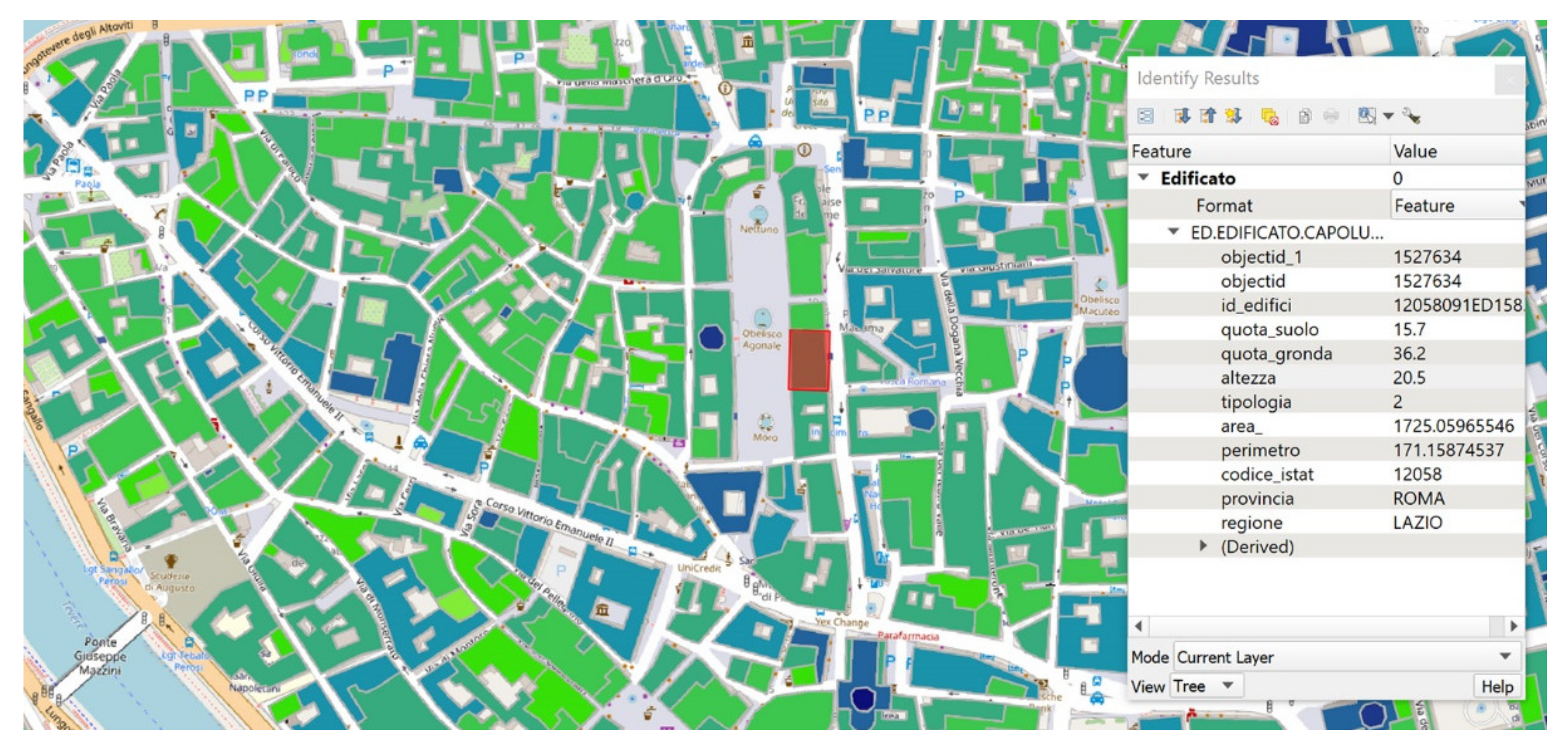
P2 evaluates the heights of the buildings, compared to the width of the OS. To extract the building heights that define the OS perimeter, a specific WFS (web feature service) layer, Edificato dei capoluoghi di provincia, was imported into the QGIS environment from Geoportale Nazionale—Ministero dell’Ambiente e della Tutela del Territorio e del Mare. With the aim of implementing the concept of the BE perimeter in GIS, we replaced each OS geometry extracted from OSM with a 10 m buffered one and performed a special intersection with the new building layer. Through the intersection among the OSM data set (with OS areas) and the MinAmbiente data set (with heights of buildings; Figure 3), for each OS, we defined P2 as follows:
P 2 = H m a x   m d 2   m
where
  • Hmax is the maximum height of the buildings that define the OS perimeter, and
  • d2 is the diameter of the maximum inscribed circumference.
P2 can assume a value smaller than one (non-critical values) or greater than one (critical values).
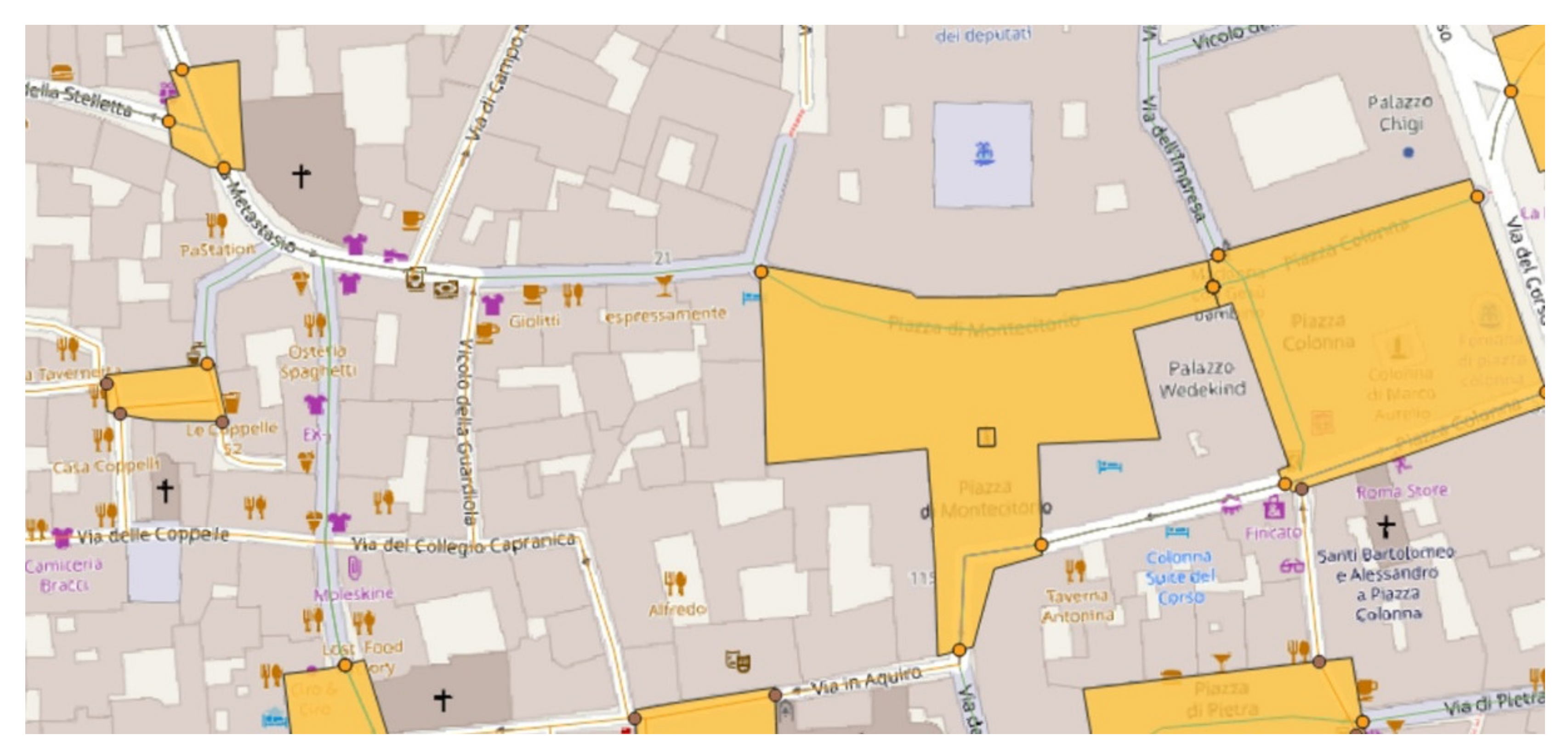
Parameter 4 evaluates the number of access points in a square, relative to the perimeter of the reference OS. Parameter 4 has been defined as the number of accesses/perimeter of an OS. To extract the BE street network, the authors formulated a specific query to the OSM database (Table 3): highway = pedestrian; highway = residential; highway = service; and highway = living_street. Indeed, in OSM, the key highway = * identifies linear geometry, and is the main key used for any kind of road, street, or path. The value of the key helps to indicate the importance of highways within the road network as a whole. The previous step is a prerequisite for the spatial analysis, where the intersection between the OS and the linear elements of the street network defines points in correspondence of the identified OS accesses (Figure 4).
To avoid overlapping duplicate points, due to a possible change of the street network name from the outside to the inside of the OS, a final merge of any point element was processed. These points inherited the attributes from the OS and the street intersection, allowing for the rapid assessment of P4, by exporting the geometric attributes in an .xls file.
P4 is defined as follows (Equation (5)):
P 4 = n u m b e r   o f   a c c e s s e s   A S   p e r i m e t e r   m
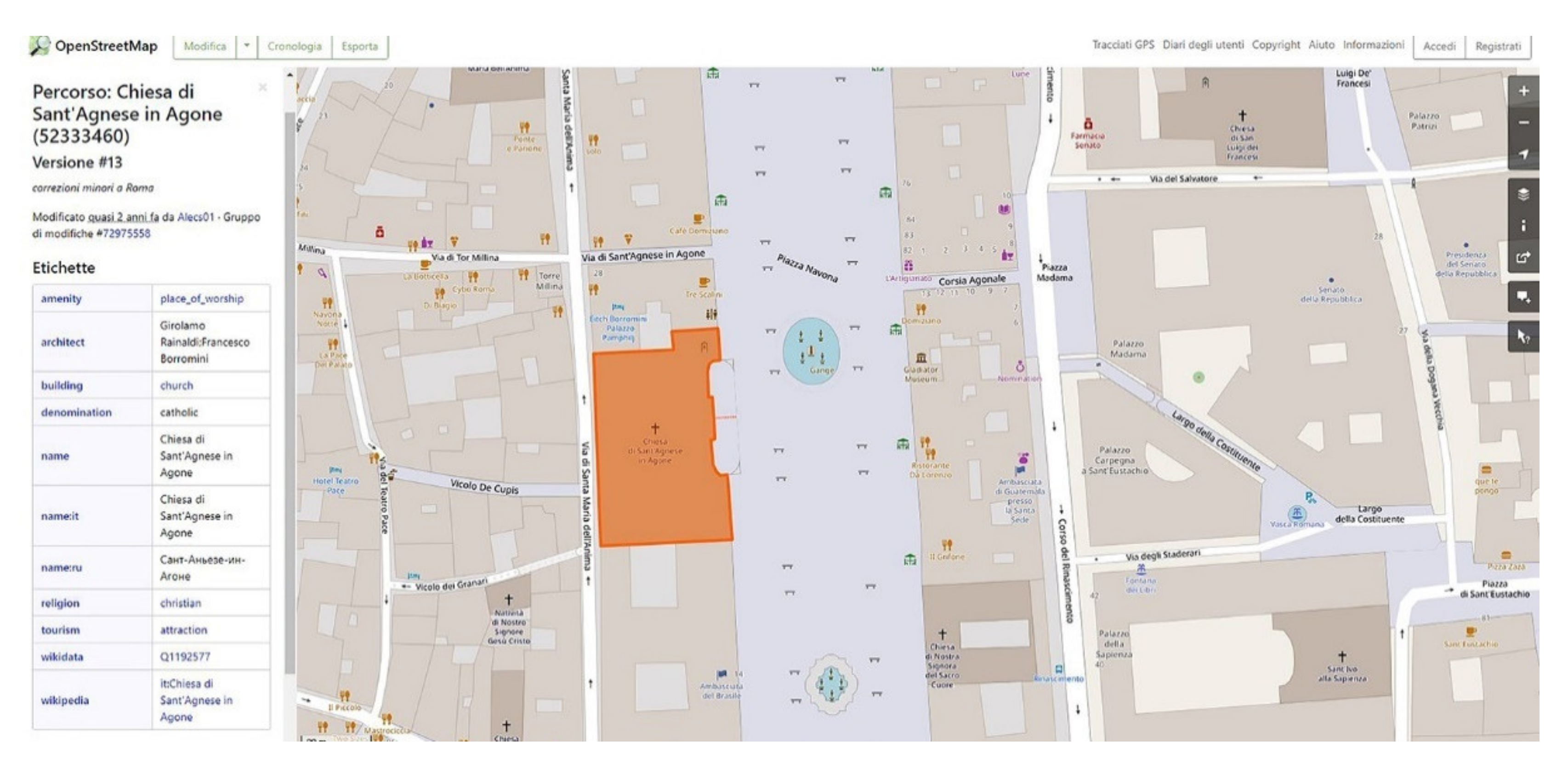
The parameter P5 indicates whether special buildings are present in the OS perimeter. To evaluate this aspect, the authors chose a suitable query (Table 3) to identify the presence of buildings dedicated to a special function, according to specific classes:
  • religious buildings (e.g., churches or other places of worship; Figure 5);
  • public buildings (e.g., town halls and police offices);
  • buildings for education (e.g., schools, colleges, and universities); and
  • buildings with cultural or tourism importance (e.g., museums, palaces, and castles).
Cleaning of the data was processed, in order to remove duplicates present in the OSM data set, caused by redundant data implementation in the OSM database [60]. Using squares and building IDs from the official MinAmbiente database, this process allowed for the removal of any supposed duplicates.
P5 is defined as follows (Equation (6)):
P 5 = n u m b e r   o f   s p e c i a l   b u i l d i n g s   i n   t h e   A S
Parameter 8 indicates the presence of a sloped ground or differences in elevation (e.g., overhangs, cliffs, and ramp/stairs). Through the information implemented in the chosen GIS database (Table 3)—and, in particular, from Edificato dei capoluoghi di provincia—we could extract the values of the minimum (HSLmin) and maximum (HSLmax) heights above sea level for each OS. In this way, it was possible to evaluate the maximum difference of height above sea level for each OS (Equation (7)):
P 8 = Δ H S L = H S L m a x m H S L m i n m
The presence of green areas is indicated by the parameter P9. We interrogated the data set, in order to verify whether any kind of green area is present within the OS considered (Figure 6). The result of this interrogation was a specification of the presence of green areas, defined by their use in the OSM database. These green areas could be of different kinds, including field surfaces, trees, and brush. It was possible to extract the overall number of OSs with green areas and the percentage of green areas in the overall OS area (Equation (8)):
P 9 = %   Green   area = g r e e n   a r e a s A S   a r e a   m 2

2.3. Cluster Analysis

A cluster analysis is a multivariate data mining technique [63,64] which has been used in several research fields, including (but not limited to) medicine, sanitary engineering, marketing, psychology, and economics. When given a large set of objects with associated data attributes, the aim is to identify groups (clusters) consisting of objects sharing a (possibly) high degree of similarity. The higher both the similarities within groups and the differences between objects belonging to different groups, the better the degree of clustering. A cluster analysis belongs to the unsupervised classification techniques: no constraint or a priori condition is imposed, and the classification derives solely from the data [35,64]. Clustering processes may be hierarchical or non-hierarchical: in the first case, a hierarchy of nested partitions (where clusters at a given level of the hierarchy include clusters of the lower levels) is built; however, in the second case, only one partition is produced by splitting the set of objects into a given number of non-overlapping clusters [65,66,67]. Considering the aim of the research, both hierarchical and non-hierarchical methods were used. As a preliminary step, to detect possible multivariate outliers in the databases, a hierarchical process based on the single-linkage method was first performed, due to the propensity of such a method for identifying objects with very different features, compared to the rest of the objects. The identification and elimination of possible multivariate outliers are crucial for the following step of clustering, as their presence heavily affects the performance of many clustering methods and the search for typological clusters.
As is usual for any agglomerative hierarchical clustering algorithm, the single-linkage method produces a cluster tree that starts with the trivial partition, where every object forms a group of its own, and continues to recursively merge the pair of current clusters which are the closest, according to some distance-based criterion (e.g., the Euclidean distance). The process continues until all objects are grouped into a single cluster [68]. Objects which remain in a cluster as singletons until the very last steps of the process turn out to be very different from the others, and may be possible multivariate outliers. After such pre-processing, in the second step of the analysis, various hierarchical and non-hierarchical algorithms are applied.
The study was intended to group BEs that share similarities, in terms of the following parameters: morphology of the OS (P1), height of their fronts related to their width (P2), number of accesses related to the OS perimeter (P4), presence of special buildings (P5), difference in height of the OS (P8), and incidence of the green areas within the OS (P9). The cluster analysis in the present research used P1, P2, P4, P8, and P9 as active variables of the process, after standardization to zero mean and unit variance (Z-scores). P5 was used as a supplementary variable during the BETs’ identification step. The parameters (P) for the OS description, as described in Section 2.1, will be referred to as variables, when used for the cluster analysis.
Various hierarchical and non-hierarchical algorithms were tested; finally, the results from the non-hierarchical k-means algorithm were chosen [63]. The k-means method assumes that every object, xi, is represented in the Euclidean space defined by data attributes. The algorithm allows for the identification of a certain number of user-defined k-clusters, represented by their centroids. Starting from k randomly chosen centroids, every object is assigned to the cluster with the closest centroid. Then, the cluster centroids are updated as the arithmetic means of the data attributes, and computed for the objects currently belonging to each cluster. The process is iterated until convergence, that is, until the centroids and the cluster memberships do not change. The distance between objects and centroids is defined in terms of the Euclidean metric; formally, the algorithm minimizes the sum of the squared errors that is used to evaluate the quality of clustering (Equation (9)):
S S E = i = 1 k x C i d i s t   c i , x 2
where k is the number of clusters, x is an object of the set, Ci is the ith cluster, ci is the centroid of cluster Ci, and dist is the Euclidean distance.
The number of clusters was chosen by taking into account two criteria: R-squared (R2) and the pseudo-F (pF) statistic [69]. The optimal number of clusters was determined by comparing the results of such two criteria: pseudo-F peaks combined with the location of a knee in the plot of the R2 against the number of clusters are generally considered as indicators of the appropriate number of clusters. Moreover, pseudo-F values provide insight into the magnitude of the discriminating power of the variables, while R2 provides a measure of separation between clusters, which are both important to obtain well-characterized typologies. The final goal of the cluster analysis is to evaluate whether the cluster profiles are meaningful and interpretable. Moreover, clusters can be further characterized on variables that were not included in the cluster analysis. A statistical analysis was performed using the SPSS Version 26.0 statistical software package [70].

2.4. From Cluster Analysis to BET Identification

Starting from the results of the cluster analysis, we identified the BETs.
The BETs were elaborated based on critical classes for parameters, through comparison of the resulting clusters. The critical classes for each parameter were set, starting from the critical analysis of the features of the OSs in BEs within each cluster, compared with the whole data set.
The mean values and the interquartile ranges of the parameters within each cluster were considered (Q1 = 25% and Q3 = 75%). According to these values, the critical classes for each parameter were elaborated in two different ways: tripartite, based on the interquartile range where meaningful differences arise (for P1), and dichotomic for the other parameters, based on their mean values. As the cluster analysis was run using only the five active variables (P1, P2, P4, P8, and P9), the supplementary variable (P5) was taken into account in the final analysis. In addition, a more detailed analysis of the relationship between critical height and OS width allowed for further investigation of the results.

3. Results

The results include the cluster analysis output and the following critical analysis performed to define the BETs. Section 3.1 describes the process used to obtain the final data set, starting from the preliminary extraction of data from the selected databases. Section 3.2 illustrates the results of the cluster analysis after the first step of cleaning of the data set by deleting the multivariate outliers, the comparison between different methods of the cluster analysis (in terms of pF and R2 values), and the output of the k-means method, chosen as the most appropriate for the present research. Then, Section 3.3 shows the critical analysis, based on the results from the k-means clustering, in order to set critical classes for each parameter. The clusters are described, through both the active variables and the supplementary variable. Finally, in Section 3.4 BETs are defined, in terms of their morphological, geometric, and functional characteristics, and a selection of real case studies matching the definition of resulting BETs is presented.

3.1. Data Set Description

The data set was composed of 1113 cases and included OSs of the capitals of the provinces of the Italian regions. Although the initial data set, extracted from OSM through the query place = square, contained 8889 cases in the entire Italian territory, only the cases also included in the MinAmbiente database were taken into account, in order to ensure data coverage for all fast analysis BET parameters (P1, P2, P4, P5, P8, and P9; Table 4). Among them, some parameters determined a further reduction of the database: it was possible to extract the information for P2 and P8 for 1392 cases, and the data relating to the computation of P4 for a total of 1113 cases; however, P5 was correctly compiled in the OSM database for 476 cases only. The small amount of cases correctly filled for P5 decreed its use as a supplementary variable, and not as an active one.
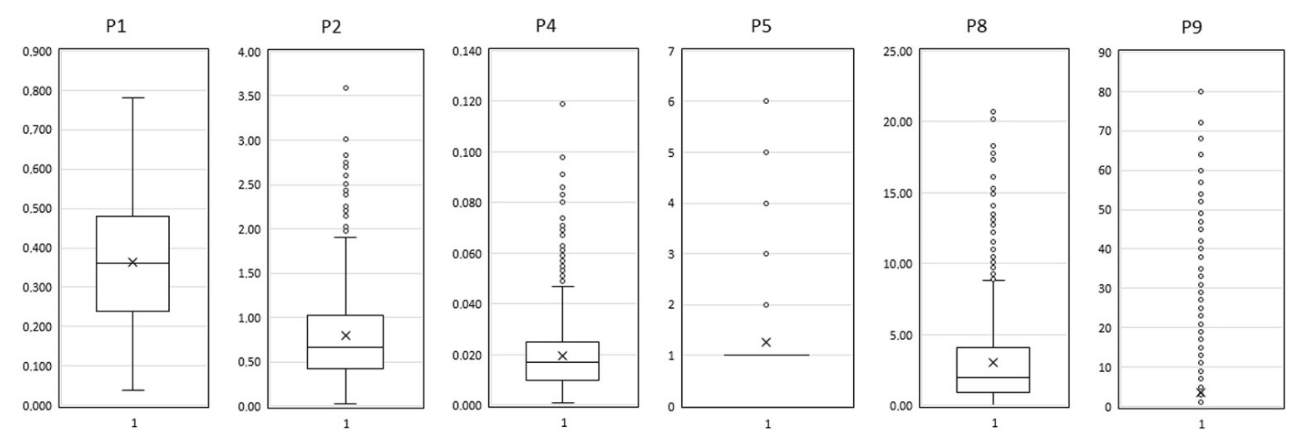
Given the nature of the data set being analysed, the parameters were divided into active (P1, P2, P4, P8, and P9) and supplementary (P5 for the cluster analysis). Their distributions presented very different patterns, in terms of variability, as is evident in Figure 7.

3.2. Cluster Analysis

The application of the single linkage method allowed for the identification of the OSs that could be assumed as multivariate outliers, as they remained non-assigned to any cluster until the very last steps of the algorithm, having characteristics very different from the rest of the OSs under study.
In this way, two cases were identified as exceptional urban spaces, in terms of their geometric dimensions and characteristics: one of them was a small widening space between dense fabrics overlooked by very tall buildings (Piazza dei Baroncelli in Florence); the other was closer to being a tree-lined avenue accessible to vehicles than a square (Piazzale Giuseppe Mazzini in Padua; Figure 8).
The two cases were eliminated from the following analysis, such that the cluster analysis was performed on the final data set, consisting of 1111 OSs.
Three hierarchical methods (Ward’s method, average linkage, and complete linkage) and the non-hierarchical method of k-means were applied to the 1111 OSs. The partitions formed by a number of clusters, varying from three to twelve groups, were selected from the results of each method, and both the pF and R2 indices were used to select the optimal partition for each method.
For each method, the pF and R2 values indicated partitioning into five clusters as the optimal solution, in terms of the similarities between OSs. Moreover, the k-means attained the maximum R2 values, which suggests that this method was the most capable of characterizing the peculiarities of the groups (Figure 9).
In Table 5, the mean values of the five parameters within each cluster from the k-means solution are reported. The mean values that differed greatly from the global mean are shown in bold, which allowed us to identify the parameters which mainly characterize each cluster. The description of single clusters will be detailed in Section 3.3.

3.3. BET Definition

The BETs were elaborated based on critical classes for parameters, through a comparison of the resulting clusters. The steps for the definition of BETs are described below.
From a critical analysis of the global mean values of the parameters, the critical classes for each parameter of the OSs were set (Table 6).
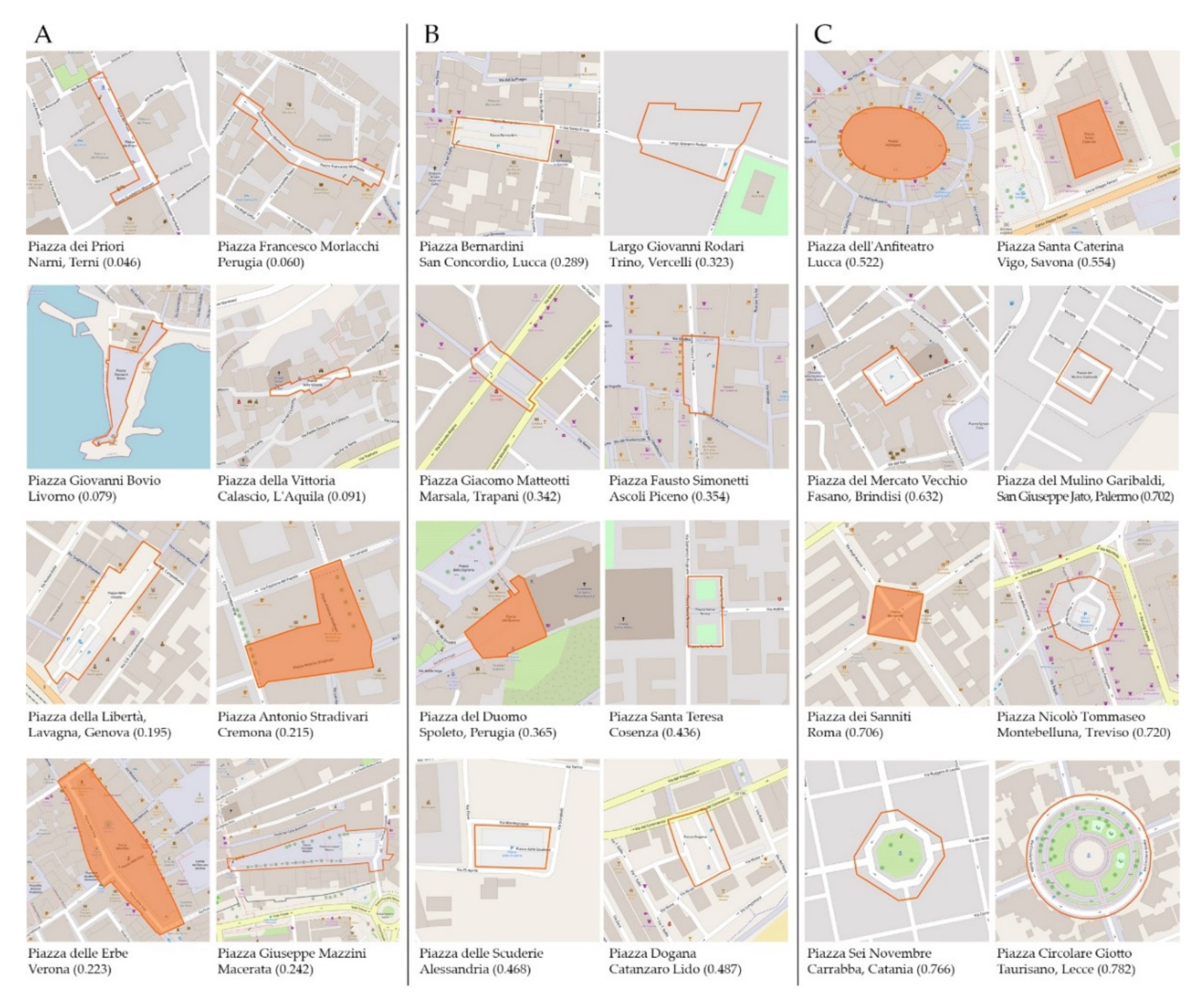
P1 was processed, both in terms of the interquartile ranges of the whole data set and the critical analysis of the features of the OSs in BEs. The tripartition of the critical classes for P1 was considered coherent with the original definition of this parameter [32], and properly described the great variety of OSs. To elaborate on the tripartition, the considered values corresponded to the 25th and 75th percentiles (equal to 0.235 and 0.476, respectively). The values were rounded up, to define threshold values equal to 0.25 and 0.50, after an inspection and checking of the data set to better represent the analysed OSs. P2 was based on the critical value equal to 1.00 (see Section 2.2), such that values above and below this threshold defined two classes. P4 and P8 were classified with reference to the global mean value. P9 was defined by a threshold value of 30% (equal to Q1 of cluster 5), representing the surface with the green area that distinguishes clusters 1, 2, 3, and 4 (not characterized by the presence of green) from cluster 5 (characterized by the presence of green). In particular, for P1, an inspection of the data set was performed to confirm the three classes highlighted by the 25th and 75th percentiles. Figure 10 shows the correspondence of the definition of P1 values, compared to the morphological classes.
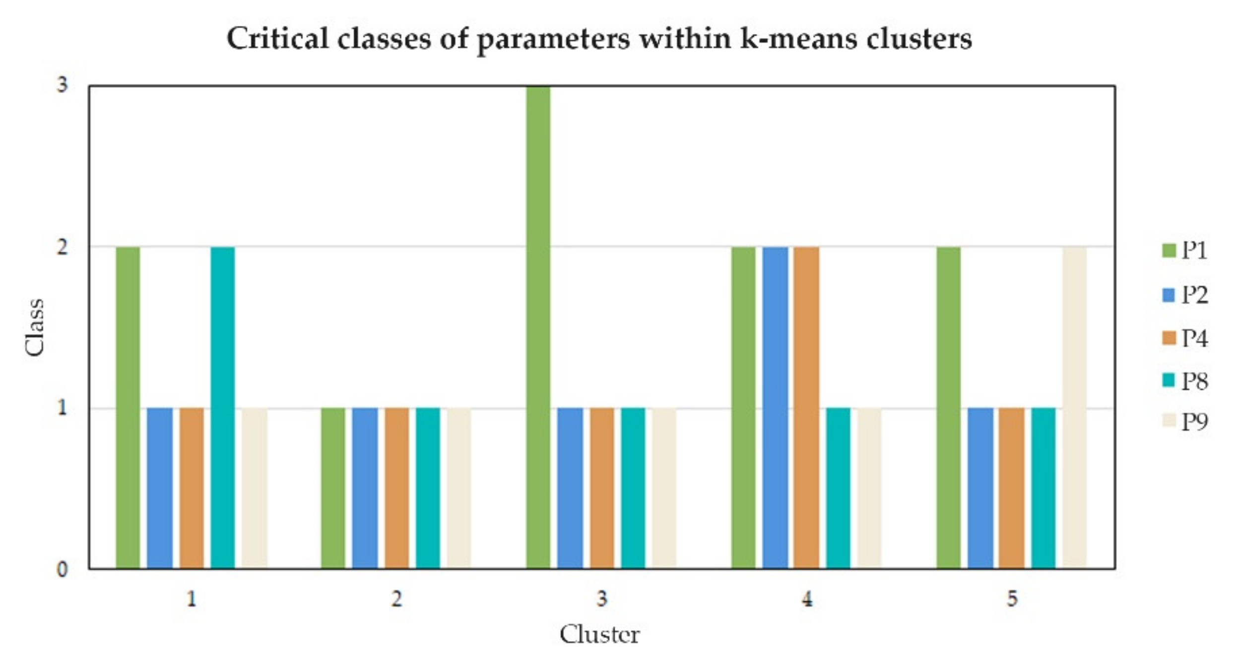
By considering the critical classes of each parameter (Table 6) in the k-means clustering, the morpho-typological and physical characterizations were described, as shown in Figure 11. This process allowed for identification of the BETs and their physical description, as illustrated in the following sections.
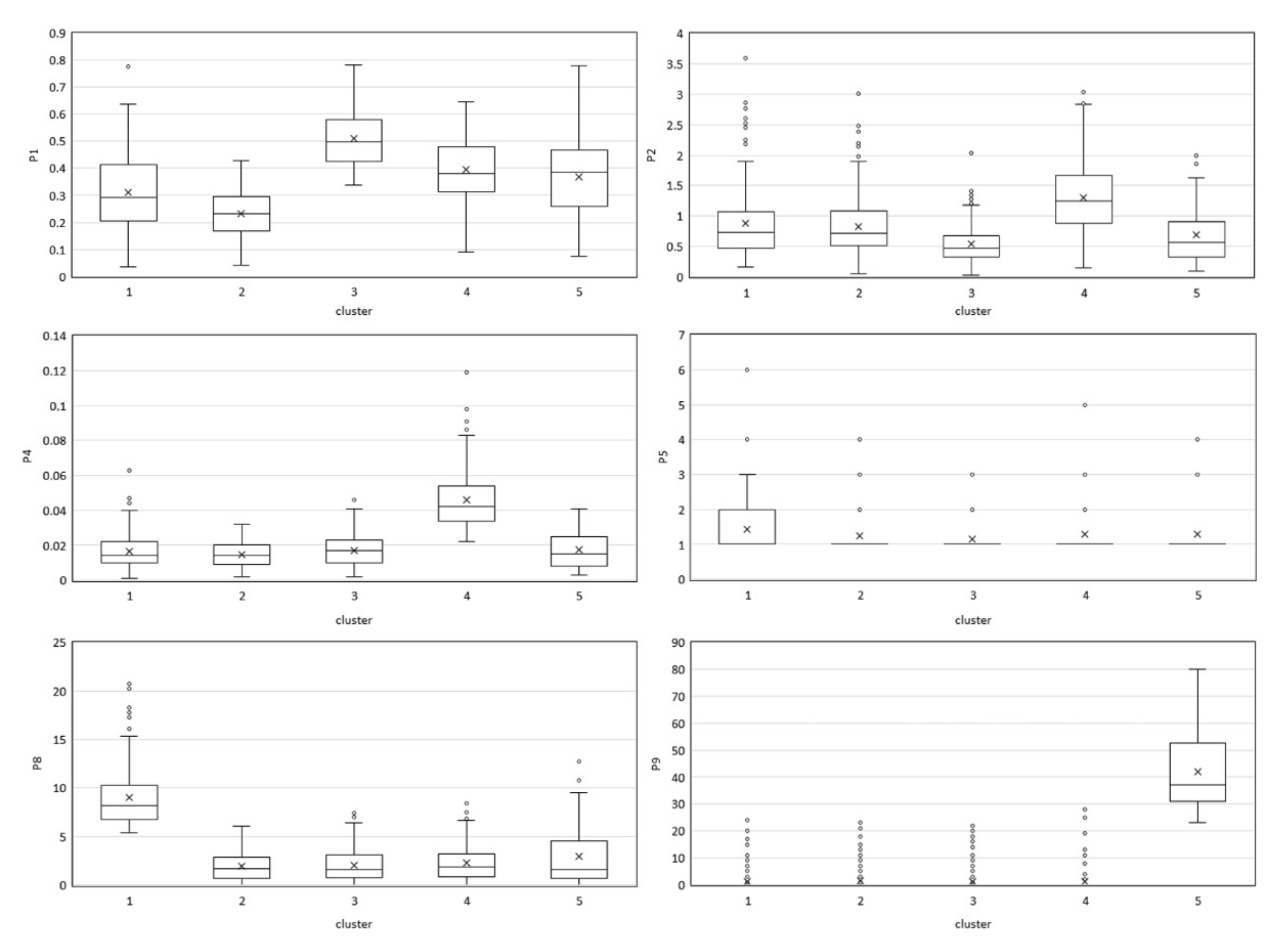
The boxplots of the parameters within each cluster are shown in Figure 12. From the boxplots, in order to describe the clusters, it is possible to compare the average values of the parameters which all exhibit low variability: P1 shows the lowest values in cluster 2 (OSs with low levels of compactness and regularity of the morphology) and the highest values in cluster 3 (OSs with high levels of compactness and regularity of the morphology); P2 shows the highest values in cluster 4 (OSs with problems of overturning for the fronts); P4 shows the highest values in cluster 4 (OSs with no critical ratio between the numbers of access and the perimeter of the OS); P5 displays the highest values in cluster 1, with a prevalence of values equal to one in the other clusters (special buildings); P8 presents the highest values in cluster 1 (OSs with the sloping ground or changes in elevation); and P9 assumes the highest values in cluster 5 (OSs with the presence of green areas). The values of the parameters are reported in Table 7.
Cluster 1: OSs with a medium level of compactness and regularity of morphology, without problems of overturning of the fronts, with a critical ratio between the number of accesses and perimeter, on sloping ground or with changes in elevation, and without green areas. The value that diverged most from the global mean is that related to the slope of the OS (P8: 9.037). Therefore, this cluster is mainly characterized by OSs with the sloping ground or with elevation changes.
Cluster 2: OSs with a low level of compactness and regularity of morphology, without problems of overturning of the fronts, with a critical ratio between the number of accesses and perimeter, on flat or slightly sloping ground, and without green areas. The value that diverges most from the global mean is that related to the morphology of the OS (P1: 0.231). Therefore, this cluster is mainly characterized by OSs with a low level of compactness and regularity of shape.
Cluster 3: OSs with a high level of compactness and regularity of morphology, without problems of overturning of the fronts, with a critical ratio between the number of accesses and perimeter, on flat or slightly sloping ground, and without green areas. The value that diverges most from the global mean is that related to the morphology of the OS (P1: 0.509). Therefore, this cluster is mainly characterized by OSs with a high level of compactness and regularity of the shape.
Cluster 4: OSs with a medium level of compactness and regularity of morphology, with problems of overturning of the fronts, without critical ratio between the number of accesses and perimeter, on flat or slightly sloping ground, and without green areas. The values that diverge most from the global means are those related to the ratio between the numbers of access and the perimeter of the OS (P4: 1.308) and the ratio between the height of the fronts and width of the OS (P2: 0.046). Therefore, this cluster is mainly characterized by OSs with problems of the overturning of the fronts, but with a suitable ratio between the number of accesses and perimeter.
Cluster 5: OSs with a medium level of compactness and regularity of morphology, without problems of overturning of the fronts, with a critical ratio between the number of accesses and perimeter, on flat or slightly sloping ground, and with green areas. The value that diverges most from the global mean is that related to the presence of green areas in the OS (P9: 0.418). Therefore, this cluster is mainly characterized by OSs with green areas.
Once the cluster analysis was performed using the active variables (P1, P2, P4, P8, and P9), the identified clusters were explored and further characterized, by analysing the supplementary variable (P5). A further analysis was also performed, in order to investigate the relationship between the height of the fronts and the width of the OS. P2 reports only the ratio of the maximum height of the built fronts to the width of the square while, in this section, a deeper investigation is reported, additionally evaluating the relationship between the median height of the fronts and the width of the OS.
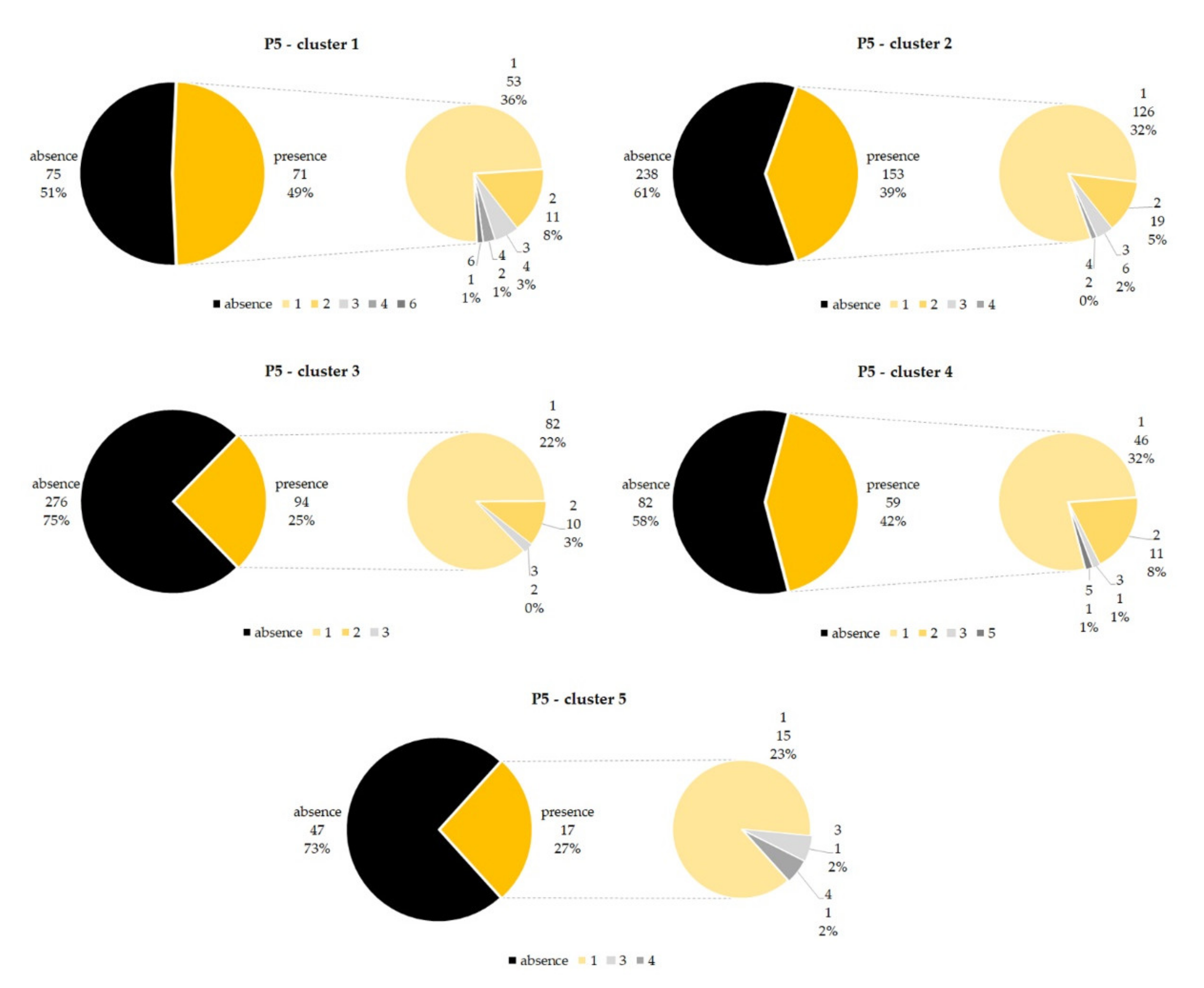
Parameter 5, which is related to the presence of special buildings in the analysed OS, is relevant for the definition of the BETs. By analysing parameter 5 within each cluster, it was possible to identify further possible subclusters. Clusters 1, 2, and 4 showed relevant percentages of OSs with the presence of special buildings (49% in cluster 1, 39% in cluster 2, and 47% in cluster 4, respectively; Figure 13). As the absence of special buildings could be linked to a lack of data in the OSM database, or to an incorrect compilation, rather than to an actual lack of special buildings, the splitting of the clusters was reasonably evaluated for the further definition of BETs.
An analysis of the relationship between the height of the built fronts and the width of the OS did not produce meaningful results, except for cluster 4, as already identified in the cluster analysis due to its high value, on average, of P2. As a consequence of this result, the values of the cases with the presence of special buildings were analysed, along with the critical heights of the built fronts. Figure 14 shows the descriptive graphs of this analysis for cluster 4, with the critical height values on the left (concerning Hmax and Hmedian values of the built fronts that define the OS perimeter) and, on the right, the same analysis is reported only for the cases with special buildings. Thus, the results obtained led us to the creation of three BETs derived from cluster 4: 4a includes at least one special building with problems of the overturning of the fronts caused by Hmax; 4b includes at least one special building with problems of the overturning of the fronts caused by Hmedian; and 4c has no special buildings but presents problems of the overturning of the fronts caused by Hmedian.

3.4. BET Representation and Real Case Studies

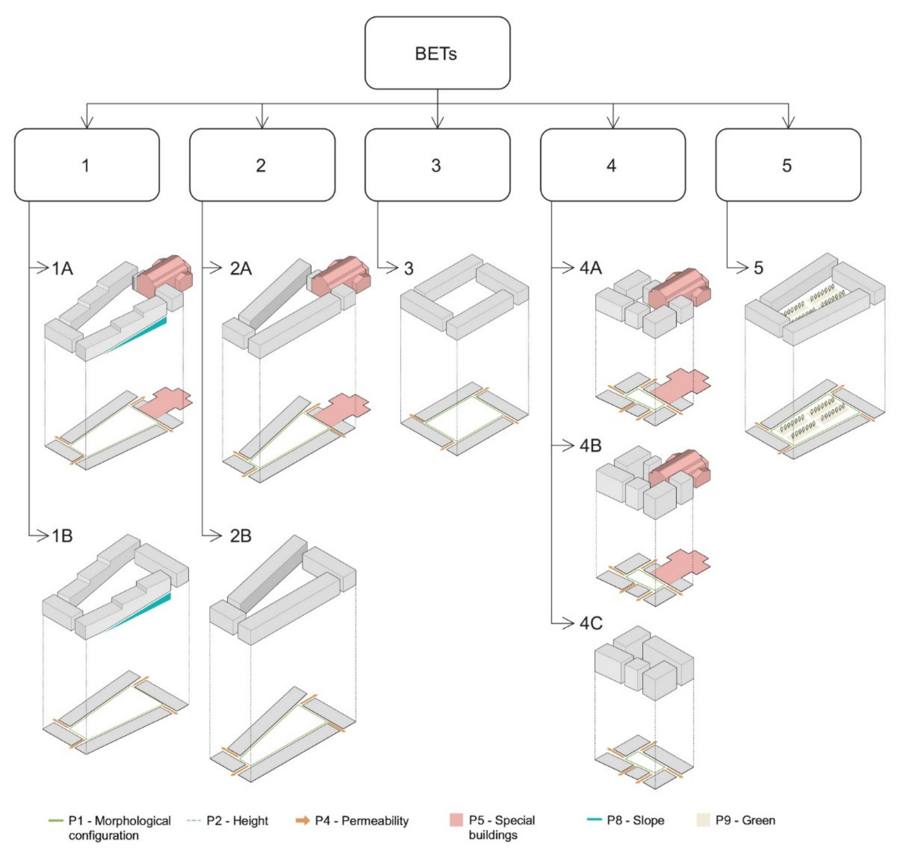
As a result of the critical analysis, nine BETs were identified. This result was derived from the combination of the cluster description and the analysis reported in Section 3.3. The diagram in Figure 15 describes the BET definitions, starting from the identified clusters.
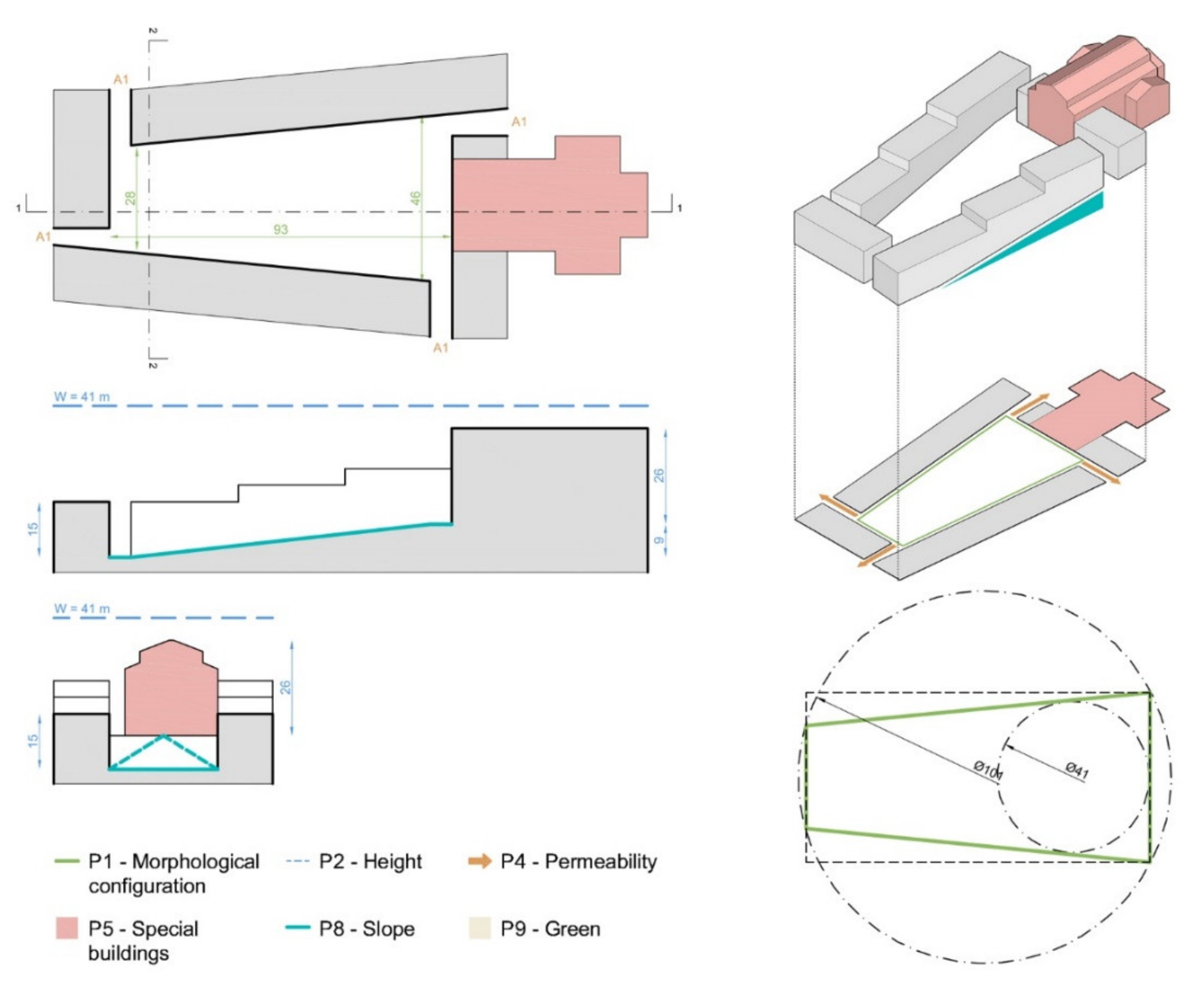
An example of a complete graphical representation for BET 1A is displayed in Figure 16, which highlights all the dimensional aspects considered for graphically representing the BETs, while Table 8 provides the dimensional values for each BET. Table 8 reports the mean values of the parameters, while the interquartile ranges are reported in parentheses.
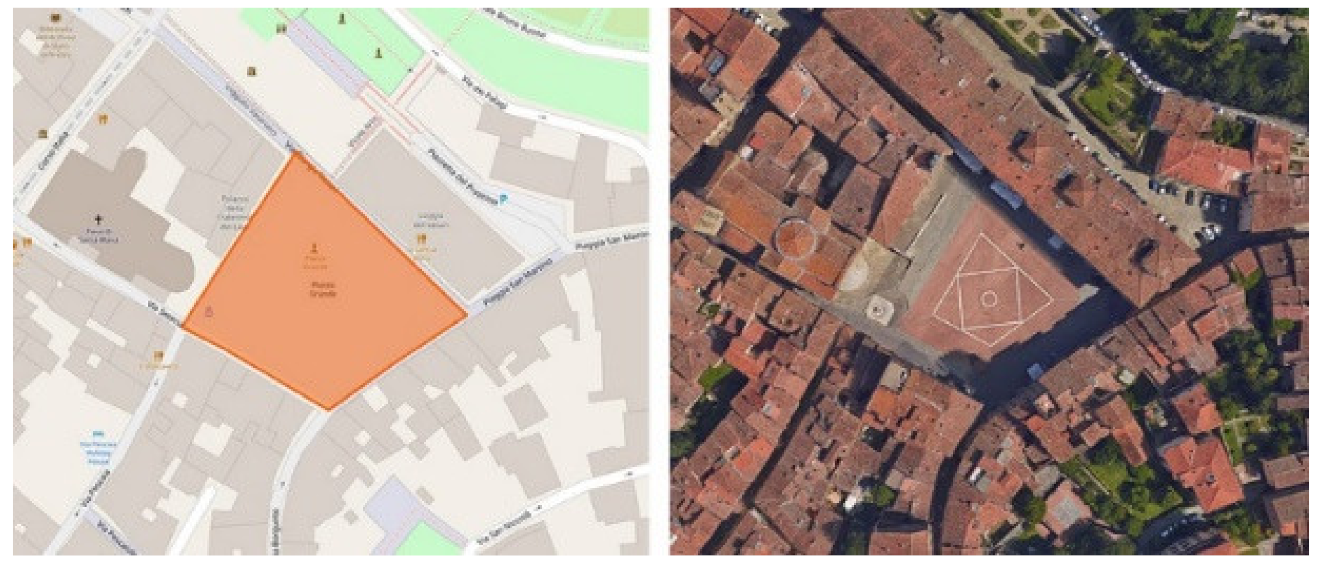
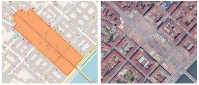
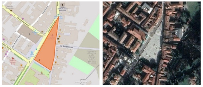
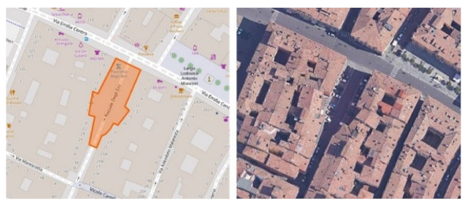
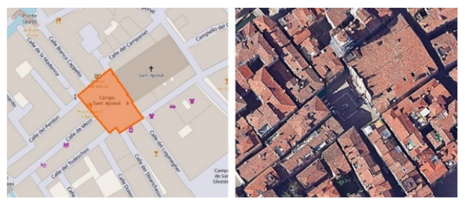
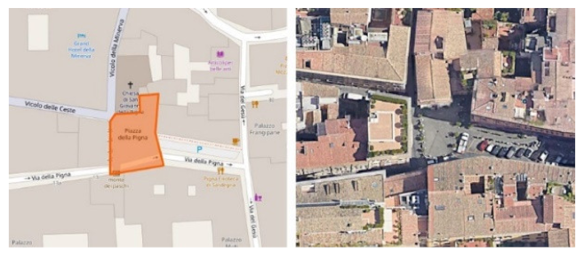
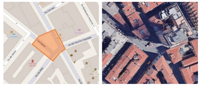
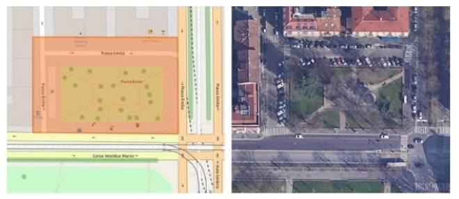
The correspondence between the idealization of BETs and real case studies was investigated for OSs in the final database. Some examples are reported in Table 9, together with the corresponding images and parameter values.

4. Discussion

4.1. From BETs towards Risk Analysis

According to the analysis, each resulting BET could be defined by a combination of characterizing risks, concerning their morphological, geometric, and functional characteristics. The analysed BEs could be affected by all the considered SUODs and SLODs; nevertheless, the specific characteristics of each BET determined their major or minor susceptibility to typical risk scenarios (Table 10).
The BETs represent typical scenarios and the basis to elaborate risk analyses. The case studies will be analysed, according to the class of the BET they belong to and, thus, to a specific risk combination. These risk combinations represent the multi-risk conditions related to analysed parameters, but not to the possibility of real overlapping of the hazards, which comprises a future step of the BE S2ECURE project. Given the parameter description against the considered SUODs and SLODs (see Section 2.1), typical risk scenarios can be proposed as follows, according to the characterizations given in Table 10.
BET 1A: No problems of overturning of the fronts (P2), thus less prone to seismic risk; presence of special buildings (P5), which implies terrorist attack risk-prone; sloping ground or ground with elevation changes (P8), serving as a possible obstacle to evacuation motion, good ventilation conditions, and pollutant transport and/or dilution; no presence of green areas (P9), thus prone to heatwaves.
BET 1B: No problems of overturning of the fronts (P2), so less prone to seismic risk; absence of special buildings (P5), thus less prone to the risk of a terrorist attack; sloping ground or ground with elevation changes (P8), serving as possible obstacles to evacuation motion, good ventilation conditions, and pollutant transport and/or dilution; no presence of green areas (P9), thus prone to heatwaves.
BET 2A: Low level of compactness and regularity of the morphology (P1), which may determine critical conditions for the evacuation paths due to debris or overcrowding during seismic events; presence of special buildings (P5), thus terrorist attack risk-prone; and no presence of green areas (P9), thus prone to heatwaves and pollution.
BET 2B: Low level of compactness and regularity of the morphology (P1), which may determine critical conditions for the evacuation paths due to debris or overcrowding during seismic events; absence of special buildings (P5), thus less prone to the risk of a terrorist attack; and no presence of green areas (P9), thus prone to heatwaves and pollution.
BET 3: High level of compactness and regularity of the morphology (P1), thus less prone to critical conditions for the evacuation paths due to debris or overcrowding during seismic events; less prone to terrorist attacks, due to an absence of special buildings (P5); and no presence of green areas (P9), thus prone to heatwaves and pollution.
BET 4A: Problems of overturning of the fronts (P2), related to the maximum height of built fronts, so more prone to seismic risk; without critical ratio between the number of accesses and perimeter (P4), so possible less critical configuration of evacuation paths and high permeability, thus higher ventilation of the space; presence of special buildings (P5), thus more terrorist attack risk-prone; and no presence of green areas (P9), thus prone to pollution, but less to heatwaves, according to the high ratio between fronts and OSs dimension (and, thus, the presence of shaded areas).
BET 4B: Problems of overturning of the fronts (P2), related to the median height of built fronts, so more prone to seismic risk; without critical ratio between the number of accesses and perimeter (P4), so possible less critical configuration of evacuation paths and high permeability, thus higher ventilation of the space; presence of special buildings (P5), thus more terrorist attack risk-prone; and no presence of green areas (P9), thus prone to pollution, but less to heatwaves, according to the high ratio between fronts and OSs dimension (and, thus, the presence of shaded areas).
BET 4C: Problems of overturning of the fronts (P2), related to the median height of built fronts, so more prone to seismic risk; without critical ratio between the number of accesses and perimeter (P4), so possible less critical configuration of evacuation paths and high permeability, thus higher ventilation of the space; less prone to terrorist attacks, due to the absence of special buildings (P5); and no presence of green areas (P9), thus prone to pollution, but less to heatwaves according to the high ratio between fronts and OSs dimension (and, thus, the presence of shaded areas).
BET 5: No problems of overturning of the fronts (P2), so less prone to seismic risk; absence of special buildings (P5), thus less terrorist attack risk-prone; and presence of green areas (P9), mitigating pollution and heatwaves.
According to these descriptions, BET 2A represents the most critically ideal scenario, being prone to the complete combination of considered risks; on the other hand, BET 5 is the least prone of the multi-risk scenarios analysed.

4.2. Limitations and Advancement in the Research Field

Although OpenStreetMap (OSM) is a valuable source of geographical data, some considerations about the limitations, in terms of data quality, should be discussed. As the maps and data editors of OSM could have different levels of experience and skills, OSM data may be vulnerable to errors and gaps. Quality issues of the OSM database are well-known [71]; therefore, using data sets extracted from OSM could be somewhat questionable. The main quality issues include: accuracy of the geometric position, completeness of the database, qualitative and quantitative information accuracy, topological consistency, and semantic accuracy.
In the context of this research, some limitations and uncertainties could be pointed out, regarding the data availability and completeness, due to the open nature of the database, and the data accuracy, affected mostly by the skill levels of editors that improve the data set, the lack of a top-down data quality assurance method, consistency of data implementation, and data source uncertainty. In particular, we highlight the incomplete data coverage for P5 (special buildings). The lack of data in a substantial portion of the data set led to its downgrading to a supplementary variable. A zero value represents, with no certainty, the absence of special buildings or the lack of available data.
Some considerations should also be made about the data extraction procedures through queries and algorithms. The reduction of queries is necessary, in order to limit both the processing time and unsuitable results; however, it resulted in a potential limitation of the cases in the data set (e.g., only the cases labelled with place = square were considered). Although the algorithms allow for an increase in data extraction, they are subject to computational errors. In particular, in the present analysis, the parameter P4 (access) was affected by data extraction problems. In fact, the number of accesses was not correctly counted when the streets were not implemented in GIS.
As is well-known, the use of the cluster analysis methodologies is affected by the method chosen and the number of clusters considered. The combined use of different methods and indicators to select the optimal partition may reduce the limitations. Moreover, the agreement of the solutions obtained by various methods indicates the presence of a clustering structure present in the data.
Although the limitations, in terms of extension and accuracy of open GIS data, have been recognized, the process proposed in this report enabled a broad evaluation of the Italian BE characteristics, due to the wide number of cases considered, reducing the time required to conduct conventional data collection. It is possible to replicate the process once the data sets considered have been implemented by OSM editors, obtaining a deeper insight into the results. Moreover, by geographically limiting the cases under study, it would be possible to obtain the characterization of the BEs of a specific Italian area. When further data sets are constructed, which describe additional aspects of the Italian BE (e.g., constructive aspects), the analysis could be repeated to include more in-depth attributes.
The definition of BETs can be further developed through the use of the parameters initially defined for a detailed analysis (P3, P6, and P7, see Section 2.1), based on the investigation of real cases. These aspects are of pivotal importance in the study of the safety of open spaces; although, they were not considered in this discussion, as there has been a lack of their implementation in databases—such as GIS ones—so far.
Finally, given the broad context of the BE S2ECURe project, such an approach could support the elaboration of specific actions for each case study, based on simulation-oriented tools, starting from the BET characteristics which it belongs to, in order to propose and evaluate tailored risk mitigation strategies. These simulation-based methods can refer to two relevant aspects: first, the estimation of disaster effects on the physical elements of the BETs; and second, the evaluation of the safety of users in BETs, depending on their disaster-affected behaviours (e.g., in SUODs, the analysis of evacuation behaviours, user motion, and their effects on safety; or, in SLODs, the analysis of users and routines affected by heatwaves or pollution scenarios). These simulation tasks can be combined in order to better stress the interactions between the BETs, their disaster-induced modifications, and the behaviours of users [16,30,31].

5. Conclusions

The identification of built environment (BE) scenarios suitable for multi-risk assessments serves as a preliminary step towards the preparation of simulation models, aimed at estimating the risk levels of open spaces (OSs) in BE and the safety of their occupants. In this context, particular attention should be paid to the specific characteristics of BEs in the Italian towns that affect sudden onset disaster (SUODs; e.g., earthquakes and terrorist attacks) and slow onset disaster (SLODs; e.g., heatwaves and air pollution) risks, taking into consideration morphological, geometric, functional, and constructive aspects. Identifying potential scenarios characterized by common Italian BE features provides the opportunity to plan further analyses and simulations for the description of risk levels.
The present work is part of an Italian PRIN (Projects of Relevant National Interest), entitled BE S2ECURe “(make) Built Environment Safer in Slow and Emergency Conditions through behavioUral assessed/designed Resilient solutions” (grant number: 2017LR75XK), supported by MIUR (the Italian Ministry of Education, University, and Research). Given the Italian context as the reference for the BE S2ECURe project, we defined typical scenarios, referring to squares as significant OSs in the urban BE. In the future steps of the BE S2ECURe project, these built environment typologies will be used for risk assessment actions, through the use of simulation-based methodologies. However, to this end, the representation of basic features referring to the morphological, functional, and physical features of such squares is the first step to be achieved, as it allows for the description of open spaces at risk (under common and typical conditions) for SUODs and SLODs. The classification provided in this work considers the different parameters that can generally affect SUODs and SLODs, as considered in the BE S2ECURe project. For the SUODs, these are earthquakes and terrorist attacks; for SLODs, heatwaves and pollution [32].
In this paper, typologies of BEs (BETs) describing multi-risk scenarios were identified, through a cluster analysis based on data extracted from GIS databases. Six parameters (P1, morphology; P2, height of the fronts; P4, number of accesses; P5, presence of special buildings; P8, slope of the ground; and P9, presence of green areas) characterizing the OSs (e.g., squares) in the BEs of existing Italian towns were selected, in order to perform fast data extraction from GIS data sets, using proper queries and algorithms.
An analysis of the final database built by the authors was carried out using five active variables (P1, P2, P4, P8, P9) and one supplementary variable (P5). The final data set included 1113 case studies, which was reduced to 1111 after the elimination of two OSs identified as multivariate outliers through use of the single-linkage method.
Several algorithms with which to perform clustering were evaluated in this study. The solution from the k-means clustering algorithm was chosen as the most appropriate to provide meaningful clusters. The results of the cluster analysis identified five groups of OSs, characterized by specific dimensional and functional characteristics. By combining the outcomes of the cluster analysis with an evaluation of the supplementary variable (P5) and a further insight on the height of the fronts (P2), nine final BETs were identified. To represent each BET, ranges of values were indicated for all parameters extracted from the data set, selecting the interquartile ranges of the values within each cluster considered (Q1 = 25% and Q3 = 75%).
Thus, the identified multi-risk scenarios comprise the basis for future risk assessments of BEs, based on statistical analyses of the peculiar characteristics of Italian towns. The results can also provide a comparative assessment of the influence of the individual features on the overall risk. The simulation-based methodologies to be applied on the BETs could consider the analysis of disaster-affected BETs, including the safety and behaviours of users under disaster conditions. The combination of such aspects will complete typical outcomes for risk assessment for each considered BET.
As already developed in similar research fields, such as structural [24,25] and energy analysis [26,27], this approach based on the idealization of the built environment lays the basis for an initial assessment on the complex issue of defining multi-risk scenarios [2,17]. The idealization of open spaces, pivotal parts of the BE for the study of risk in the urban environment [12,20], represents a step towards a comparison of risk simulation results, not only linked to the specificities of the case studies, but also to set a shared methodology for BE investigation. Being aware of the necessary approximations to set up BE performance simulations, the approach allows for an initial analysis based on essential parameters for the description of BE. The characteristics considered allow understanding of the fragility of the BE prone to individual risks and combinations of these, to be further evaluated with respect to the real hazards present in specific case studies, both analysed in the BE S2ECURe project and in other similar research focusing on BEs.

Author Contributions

Conceptualization of the research, E.C., A.D., M.R., M.A. and E.Q.; conceptualization of the paper, A.D. and M.R.; methodology, A.D., M.R., M.A., D.V. and E.C.; validation, G.B., E.Q., D.V., A.D., M.R. and E.C.; GIS formal analysis, M.A.; statical analysis, A.D.; investigation, M.R.; data curation, A.D. and M.R.; writing—original draft preparation, A.D. [Section 1, Section 2, Section 2.3, Section 2.4, Section 3, Section 3.2, Section 3.3, Section 4], M.R. [Section 2, Section 2.1, Section 2.4, Section 3, Section 3.3, Section 3.4, Section 4, Section 5] and M.A. [§ 2.2, 3.1]; writing—review and editing, A.D., M.R., M.A., D.V. and E.C.; GIS visualization, M.A.; data visualization A.D. and M.R.; supervision, D.V. (statistics), E.C. (building architecture); project administration, G.B., E.C. and E.Q.; funding acquisition, E.Q. and E.C. All authors have read and agreed to the published version of the manuscript.

Funding

This research was funded by the MIUR (the Italian Ministry of Education, University, and Research) Project BE S2ECURe—(make) Built Environment Safer in Slow and Emergency Conditions through behavioUral assessed/designed Resilient solutions (grant number: 2017LR75XK).

Institutional Review Board Statement

Not applicable.

Informed Consent Statement

Not applicable.

Data Availability Statement

The data presented in this study are available online on the website of the Project BE S2ECURe: https://en.bes2ecure.net/ https://en.bes2ecure.net/wp3.

Conflicts of Interest

The authors declare no conflict of interest.

References

  1. Scolobig, A.; Garcia-aristizabal, A.; Komendantova, N.; Patt, A.; Ruocco, A.D.; Gasparini, P.; Monfort, D.; Vinchon, C.; Mrzy, R.; Fleming, K.; et al. From Multi-Risk Assessment to Multi-Risk Governance: Recommendations for Future Directions. In Understanding Risk: The Evolution of Disaster Risk Assessment; GFDRR, Ed.; International Bank for reconstruction and Development: Washington, DC, USA, 2015; pp. 163–167. [Google Scholar]
  2. Komendantova, N.; Mrzyglocki, R.; Mignan, A.; Khazai, B.; Wenzel, F.; Patt, A.; Fleming, K. Multi-hazard and multi-risk decision-support tools as a part of participatory risk governance: Feedback from civil protection stakeholders. Int. J. Disaster Risk Reduct. 2014, 8, 50–67. [Google Scholar] [CrossRef] [Green Version]
  3. Dilley, M.; Chen, R.S.; Deichmann, U.; Lerner-Lam, A.L.; Arnold, M. Natural Disaster Hotspots: A Global Risk Analysis; World Bank: Washington, DC, USA, 2005. [Google Scholar]
  4. IPCC. Managing the Risks of Extreme Events and Disasters to Advance Climate Change Adaptation; Intergovernmental Panel On Climate Change, Ed.; Cambridge University Press: Cambridge, UK, 2012; Volume 9781107025, ISBN 9781139177245. [Google Scholar]
  5. WHO. Definitions: Emergencies. Available online: https://www.who.int/hac/about/definitions/en/ (accessed on 29 November 2019).
  6. PreventionWeb—UNDRR. Available online: https://www.preventionweb.net/terminology#D (accessed on 2 October 2020).
  7. UNISDR. Sendai Framework for Disaster Risk Reduction 2015–2030; United Nations Office for Disaster Risk Reduction: Geneva, Switzerland, 2015; Available online: http://www.unisdr.org/files/43291_sendaiframeworkfordrren.pdf (accessed on 1 September 2020).
  8. Kappes, M.S.; Keiler, M.; von Elverfeldt, K.; Glade, T. Challenges of analyzing multi-hazard risk: A review. Nat. Hazards 2012, 64, 1925–1958. [Google Scholar] [CrossRef] [Green Version]
  9. Gallina, V.; Torresan, S.; Critto, A.; Sperotto, A.; Glade, T.; Marcomini, A. A review of multi-risk methodologies for natural hazards: Consequences and challenges for a climate change impact assessment. J. Environ. Manag. 2016, 168, 123–132. [Google Scholar] [CrossRef]
  10. Sharifi, A. Urban form resilience: A meso-scale analysis. Cities 2019, 93, 238–252. [Google Scholar] [CrossRef]
  11. Russo, M.; Angelosanti, M.; Bernardini, G.; Cantatore, E.; D’Amico, A.; Currà, E.; Fatiguso, F.; Mochi, G.; Quagliarini, E. Morphological Systems of Open Spaces in Built Environment Prone to Sudden-Onset Disasters. In Sustainability in Energy and Buildings 2020 (Part of the Smart Innovation, Systems and Technologies Book Series—SIST, Volume 203—ISSN: 2190–3018); Littlewood, J., Howlett, R.J., Jain, L.C., Eds.; Springer: Singapore, 2021; pp. 321–331. ISBN 978-981-15-8783-2. [Google Scholar]
  12. French, E.L.; Birchall, S.J.; Landman, K.; Brown, R.D. Designing public open space to support seismic resilience: A systematic review. Int. J. Disaster Risk Reduct. 2019, 34, 1–10. [Google Scholar] [CrossRef] [Green Version]
  13. Arosio, M.; Martina, M.L.V.; Figueiredo, R. The whole is greater than the sum of its parts: A holistic graph-based assessment approach for natural hazard risk of complex systems. Nat. Hazards Earth Syst. Sci. 2020, 20, 521–547. [Google Scholar] [CrossRef] [Green Version]
  14. Gill, J.C.; Malamud, B.D. Hazard interactions and interaction networks (cascades) within multi-hazard methodologies. Earth Syst. Dyn. 2016, 7, 659–679. [Google Scholar] [CrossRef] [Green Version]
  15. Mignan, A.; Wiemer, S.; Giardini, D. The quantification of low-probability-high-consequences events: Part I. A generic multi-risk approach. Nat. Hazards 2014, 73, 1999–2022. [Google Scholar] [CrossRef] [Green Version]
  16. Bernardini, G.; Romano, G.; Soldini, L.; Quagliarini, E. How urban layout and pedestrian evacuation behaviours can influence flood risk assessment in riverine historic built environments. Sustain. Cities Soc. 2021, 70, 102876. [Google Scholar] [CrossRef]
  17. White, G.F.; Kates, R.W.; Burton, I. Knowing better and losing even more: The use of knowledge in hazards management. Environ. Hazards 2001, 3, 81–92. [Google Scholar] [CrossRef] [Green Version]
  18. Dunant, A.; Bebbington, M.; Davies, T.; Horton, P. Multihazards Scenario Generator: A Network-Based Simulation of Natural Disasters. Risk Anal. 2021. [Google Scholar] [CrossRef]
  19. Schmidt, J.; Matcham, I.; Reese, S.; King, A.; Bell, R.; Henderson, R.; Smart, G.; Cousins, J.; Smith, W.; Heron, D. Quantitative multi-risk analysis for natural hazards: A framework for multi-risk modelling. Nat. Hazards 2011, 58, 1169–1192. [Google Scholar] [CrossRef]
  20. Koren, D.; Rus, K. The potential of open space for enhancing urban seismic resilience: A literature review. Sustainability 2019, 11, 5942. [Google Scholar] [CrossRef] [Green Version]
  21. Russo, M.; Angelosanti, M.; Bernardini, G.; Cantatore, E.; D’Amico, A.; Currà, E.; Fatiguso, F.; Mochi, G.; Quagliarini, E. Morphological systems of open spaces in built environment prone to Sudden-onset disasters. In Proceedings of the International Conference on Sustainability in Energy and Buildings SEB 2020, Split, Croatia, 24–26 June 2020; pp. 1–10. [Google Scholar]
  22. Quagliarini, E.; Lucesoli, M.; Bernardini, G. How to create seismic risk scenarios in historic built environment using rapid data collection and managing. J. Cult. Herit. 2021, 48, 93–105. [Google Scholar] [CrossRef]
  23. Mandolesi, E.; Ferrero, A. Piazze del Piceno; Gangemi: Rome, Italy, 2001; ISBN 9788849201307. [Google Scholar]
  24. Zuccaro, G.; Dolce, M.; De Gregorio, D.; Speranza, E.; Moroni, C. La Scheda Cartis Per La Caratterizzazione Tipologico- Strutturale Dei Comparti Urbani Costituiti Da Edifici Ordinari. Valutazione dell’esposizione in analisi di rischio sismico. In Proceedings of the 39th National Conference of the National Group of Geophysics of the Solid Earth GNGTS 2015 (Gruppo Nazionale di Geofisica della Terra Solida), Trieste, Italy, 17–19 November 2015; pp. 281–287. [Google Scholar]
  25. Dolce, M.; Prota, A.; Borzi, B.; da Porto, F.; Lagomarsino, S.; Magenes, G.; Moroni, C.; Penna, A.; Polese, M.; Speranza, E.; et al. Seismic Risk Assessment of Residential Buildings in Italy; Springer: Dordrecht, The Netherlands, 2020; ISBN 0123456789. [Google Scholar]
  26. Morganti, M.; Salvati, A.; Coch, H.; Cecere, C. Urban morphology indicators for solar energy analysis. Energy Procedia 2017, 134, 1–8. [Google Scholar] [CrossRef]
  27. Morganti, M. Spatial Metrics to Investigate the Impact of Urban Form on Microclimate and Building Energy Performance: An Essential Overview. In Urban Microclimate Modelling for Comfort and Energy Studies; Palme, M., Salvati, A., Eds.; Springer: Cham, Germany, 2021; pp. 385–402. [Google Scholar]
  28. Mignot, E.; Li, X.; Dewals, B. Experimental modelling of urban flooding: A review. J. Hydrol. 2019, 568, 334–342. [Google Scholar] [CrossRef] [Green Version]
  29. Ronchi, E.; Kuligowski, E.D.; Reneke, P.A.; Peacock, R.D.; Nilsson, D. The Process of Verification and Validation of Building Fire Evacuation Models. NIST Tech. Note 2013, 1822, 84. [Google Scholar]
  30. Lovreglio, R.; Ronchi, E.; Maragkos, G.; Beji, T.; Merci, B. A dynamic approach for the impact of a toxic gas dispersion hazard considering human behaviour and dispersion modelling. J. Hazard. Mater. 2016, 318, 758–771. [Google Scholar] [CrossRef]
  31. Cimellaro, G.P.; Ozzello, F.; Vallero, A.; Mahin, S.; Shao, B. Simulating earthquake evacuation using human behavior models. Earthq. Eng. Struct. Dyn. 2017, 46, 985–1002. [Google Scholar] [CrossRef]
  32. BE S2ECURE project D 3.1.1 | BETs Definition and Representation Report; 2021; Working Report (draft) from BE S2ECURe “(make) Built Environment Safer in Slow and Emergency Conditions through BehavioUral Assessed/Designed Resilient Solutions” Research Project. Available online: http://bit.ly/bes2ecure_D311 (accessed on 31 May 2021).
  33. Tate, N.J.; Fisher, P.F.; Martin, D.J. Geographic Information Systems and Surfaces. In The Handbook of Geographic Information Science; Blackwell Publishing: Malden, MA, USA, 2008; pp. 239–258. [Google Scholar] [CrossRef]
  34. Zhou, C.; Wu, Y. A planning support tool for layout integral optimization of urban blue-green infrastructure. Sustainability 2020, 12, 1613. [Google Scholar] [CrossRef] [Green Version]
  35. Paliaga, G.; Faccini, F.; Luino, F.; Roccati, A.; Turconi, L. A clustering classification of catchment anthropogenic modification and relationships with floods. Sci. Total Environ. 2020, 740, 139915. [Google Scholar] [CrossRef]
  36. Sharifi, A. Resilient urban forms: A review of literature on streets and street networks. Build. Environ. 2019, 147, 171–187. [Google Scholar] [CrossRef]
  37. Yıldız, B.; Çağdaş, G. Fuzzy logic in agent-based modeling of user movement in urban space: Definition and application to a case study of a square. Build. Environ. 2020, 169, 106597. [Google Scholar] [CrossRef]
  38. Shrestha, S.R.; Sliuzas, R.; Kuffer, M. Open spaces and risk perception in post-earthquake Kathmandu city. Appl. Geogr. 2018, 93, 81–91. [Google Scholar] [CrossRef]
  39. Ghiaus, C.; Allard, F.; Santamouris, M.; Georgakis, C.; Nicol, F. Urban environment influence on natural ventilation potential. Build. Environ. 2006, 41, 395–406. [Google Scholar] [CrossRef]
  40. Cao, J.; Zhu, J.; Zhang, Q.; Wang, K.; Yang, J.; Wang, Q. Modeling urban intersection form: Measurements, patterns, and distributions. Front. Archit. Res. 2020, 10, 33–49. [Google Scholar] [CrossRef]
  41. Zhou, Y.; Levy, J. The impact of urban street canyons on population exposure to traffic-related primary pollutants. Atmos. Environ. 2008, 42, 3087–3098. [Google Scholar] [CrossRef]
  42. Salvalai, G.; Moretti, N.; Blanco Cadena, J.D.; Quagliarini, E. SLow Onset Disaster Events Factors in Italian Built Environment Archetypes. In Sustainability in Energy and Buildings 2020; Springer: Singapore, 2021; pp. 333–343. [Google Scholar]
  43. Wagner, N.; Agrawal, V. An agent-based simulation system for concert venue crowd evacuation modeling in the presence of a fire disaster. Expert Syst. Appl. 2014, 41, 2807–2815. [Google Scholar] [CrossRef]
  44. FEMA-426/BIPS-06 Reference Manual to Mitigate Potential Terrorist Attacks Against Buildings. FEMA-426/BIPS-06 Ed. 2; Federal Emergency Management Agency, Department of Homeland Security, Science and Technology Directorate, Infrastructure Protection and Disaster Management Division: Washington, DC, USA, 2011; Volume 510. Available online: https://www.dhs.gov/xlibrary/assets/st/st-bips-06.pdf (accessed on 1 September 2020).
  45. FEMA 430: Federal Emergency Management Agency. Site and Urban Design for Security: Guidance Against Potential Terrorist Attacks 2007. Department of Homeland Security: Washington, DC, USA; Available online: https://www.wbdg.org/FFC/DHS/fema430.pdf (accessed on 1 September 2020).
  46. Khamis, N.; Selamat, H.; Ismail, F.S.; Lutfy, O.F.; Haniff, M.F.; Nordin, I.N.A.M. Optimized exit door locations for a safer emergency evacuation using crowd evacuation model and artificial bee colony optimization. Chaos Solitons Fractals 2020, 131, 109505. [Google Scholar] [CrossRef]
  47. Italian Technical Commission for Seismic Micro-zoning. Handbook of Analysis of Emergency Conditions in Urban Scenarios (Manuale per L’analisi Della Condizione Limite Dell’emergenza Dell’insediamento Urbano (CLE), 1st ed.; Bramerini, F., Castenetto, S., Eds.; (in Italian). BetMultimedia: Rome, Italy, 2014; ISBN 978-88-97457-00-8. [Google Scholar]
  48. Artese, S.; Achilli, V. A gis tool for the management of seismic emergencies in historical centers: How to choose the optimal routes for civil protection interventions. ISPRS Int. Arch. Photogramm. Remote Sens. Spat. Inf. Sci. 2019, XLII-2/W11, 99–106. [Google Scholar] [CrossRef] [Green Version]
  49. Zlateski, A.; Lucesoli, M.; Bernardini, G.; Ferreira, T.M. Integrating human behaviour and building vulnerability for the assessment and mitigation of seismic risk in historic centres: Proposal of a holistic human-centred simulation-based approach. Int. J. Disaster Risk Reduct. 2020, 43, 101392. [Google Scholar] [CrossRef]
  50. CFPA Europe Confederation of Fire Protection Associations Europe. Fire Safety Engineering Concerning Evacuation from Buildings—Guidelines No 19:2009; Confederation of Fire Protection Associations in Europe (CFPA E): Zurich, Switzerland, 2009; Available online: https://www.cfpa-e.eu/wp-content/uploads/files/guidelines/CFPA_E_Guideline_No_19_2009.pdf (accessed on 1 September 2020).
  51. Blanco Cadena, J.D.; Salvalai, G.; Lucesoli, M.; Quagliarini, E.; D’Orazio, M. Flexible Workflow for Determining Critical Hazard and Exposure Scenarios for Assessing SLODs Risk in Urban Built Environments. Sustainability 2021, 13, 4538. [Google Scholar] [CrossRef]
  52. Rosso, F.; Golasi, I.; Castaldo, V.L.; Piselli, C.; Pisello, A.L.; Salata, F.; Ferrero, M.; Cotana, F.; de Lieto Vollaro, A. On the impact of innovative materials on outdoor thermal comfort of pedestrians in historical urban canyons. Renew. Energy 2018, 118, 825–839. [Google Scholar] [CrossRef]
  53. Falasca, S.; Ciancio, V.; Salata, F.; Golasi, I.; Rosso, F.; Curci, G. High albedo materials to counteract heat waves in cities: An assessment of meteorology, buildings energy needs and pedestrian thermal comfort. Build. Environ. 2019, 163, 106242. [Google Scholar] [CrossRef]
  54. D’Orazio, M.; Spalazzi, L.; Quagliarini, E.; Bernardini, G. Agent-based model for earthquake pedestrians’ evacuation in urban outdoor scenarios: Behavioural patterns definition and evacuation paths choice. Saf. Sci. 2014, 62, 450–465. [Google Scholar] [CrossRef]
  55. Shiwakoti, N.; Shi, X.; Ye, Z. A review on the performance of an obstacle near an exit on pedestrian crowd evacuation. Saf. Sci. 2019, 113, 54–67. [Google Scholar] [CrossRef]
  56. Santamouris, M.; Ban-Weiss, G.; Osmond, P.; Paolini, R.; Synnefa, A.; Cartalis, C.; Muscio, A.; Zinzi, M.; Morakinyo, T.E.; Ng, E.; et al. Progress in urban greenery mitigation science—Assessment methodologies advanced technologies and impact on cities. J. Civ. Eng. Manag. 2018, 24, 638–671. [Google Scholar] [CrossRef] [Green Version]
  57. FAO. Building greener cities: Nine benefits of urban trees. Food and Agriculture Organisation of the United Nations: Rome. Available online: http://www.fao.org/zhc/detail-events/en/c/454543/ (accessed on 1 September 2020).
  58. ArcGIS GIS Dictionary. Available online: https://support.esri.com/en/other-resources/gis-dictionary (accessed on 2 October 2020).
  59. QGIS.org. QGIS Geographic Information System. Available online: http://www.qgis.org (accessed on 2 October 2020).
  60. Mooney, P.; Minghini, M. A Review of OpenStreetMap Data. In Mapping and the Citizen Sensor; Foody, G., See, L., Fritz, S., Mooney, P., Olteanu-Raimond, A.-M., Fonte, C.C., Antoniou, V., Eds.; Ubiquity Press: London, UK, 2017; pp. 37–59. [Google Scholar]
  61. Agafonkin, V. A New Algorithm for Finding a Visual Center of a Polygon. Available online: https://blog.mapbox.com/a-new-algorithm-for-finding-a-visual-center-of-a-polygon-7c77e6492fbc (accessed on 4 January 2021).
  62. Garcia-Castellanos, D.; Lombardo, U. Poles of inaccessibility: A calculation algorithm for the remotest places on earth. Scott. Geogr. J. 2007, 123, 227–233. [Google Scholar] [CrossRef]
  63. MacQueen, J.B. Some methods for classification and analysis of multivariate observations. In Proceedings of the Fifth Berkeley Symposium on Mathematical Statistics and Probability, Berkeley, CA, USA, 21 June–18 July 1965; University of California Press: Berkeley, CA, USA, 1967; Volume 1, pp. 281–297. [Google Scholar]
  64. Halkidi, M. On Clustering Validation Techniques. J. Intell. Inf. Syst. 2001, 17, 107–145. [Google Scholar] [CrossRef]
  65. Hartigan, J.A. Clustering Algorithms, 99th ed.; John Wiley&Sons, Inc.: Hoboken, NJ, USA, 1975; ISBN 047135645X. [Google Scholar]
  66. Landau, S.; Chis Ster, I. Cluster Analysis: Overview. In International Encyclopedia of Education, 3rd ed.; Peterson, P., Baker, E., McGaw, B., Eds.; Elsevier: Amsterdam, The Netherlands, 2010; pp. 72–83. [Google Scholar]
  67. Everitt, B.; Landau, S.; Leese, M.; Stahl, D. Cluster Analysis, 5th ed.; Wiley: Chichester, UK, 2011. [Google Scholar]
  68. Satari, S.Z.; Muhammad Di, N.F.; Zakaria, R. The multiple outliers detection using agglomerative hierarchical methods in circular regression model. J. Phys. Conf. Ser. 2017, 890, 12152. [Google Scholar] [CrossRef] [Green Version]
  69. Calinski, T.; Harabasz, J. A dendrite method for cluster analysis. Commun. Stat. 1974, 3, 1–27. [Google Scholar]
  70. IBM Corp. IBM SPSS Statistics for Windows, version 26; IBM Corp.: Armonk, NY, USA, 2019. [Google Scholar]
  71. Kaur, J.; Singh, J.; Sehra, S.S.; Rai, H.S. Systematic literature review of data quality within openstreetmap. In Proceedings of the 2017 International Conference on Next Generation Computing and Information Systems (ICNGCIS), Jammu, India, 11–12 December 2017; pp. 159–163. [Google Scholar] [CrossRef]
Figure 1. Representation of the methodology workflow: identification of databases, importing into GIS software, data query concept, data extraction, descriptive statistical analysis of data, and cluster analysis for BETs identification.
Sustainability 13 09457 g001
Figure 2. Italian OS layer extraction from OSM, performed by authors through the query “place = square” (in orange).
Sustainability 13 09457 g002
Figure 3. Italian principal city building height extraction from the MinAmb database.
Sustainability 13 09457 g003
Figure 4. Example of accesses identified through the intersection between the layers of OS and street network from the OSM database.
Sustainability 13 09457 g004
Figure 5. Example of the query “amenity = place_of_worship” to identify the religious building on the OS perimeter from the OSM database.
Sustainability 13 09457 g005
Figure 6. Example of a green area (query leisure = park) within an OS; Piazza Vittorio, Roma.
Sustainability 13 09457 g006
Figure 7. Boxplots of the parameters of the final data set (1113 cases). ×: mean value; line: median value; o: univariate outliers.
Sustainability 13 09457 g007
Figure 8. Multivariate outliers: Piazza dei Baroncelli in Florence (on the left) and Piazzale Giuseppe Mazzini in Padua (on the right).
Sustainability 13 09457 g008
Figure 9. Values of pF and R2 across the number of clusters from five different methods of cluster analyses.
Sustainability 13 09457 g009
Figure 10. Examples of the OSs belonging to the three classes of P1 (Table 7). Images from OpenStreetMaps. (A) Class 1, low level of compactness and regularity. (B) Class 2, medium level of compactness and regularity. (C) Class 3, high level of compactness and regularity.
Sustainability 13 09457 g010
Figure 11. Cluster characterizations through the parameter thresholds reported in Table 6: k-means clusters on the x-axis, critical classes of parameters on the y-axis.
Sustainability 13 09457 g011
Figure 12. Boxplots of the parameter values within clusters (×: mean value; line: median value; box: Q1 and Q3; ◦: univariate outliers). P1, P2, P5, and P8 are adimensional data, P4 [m−1], and P9 [%].
Sustainability 13 09457 g012
Figure 13. Analysis of the supplementary variable (P5) within clusters.
Sustainability 13 09457 g013
Figure 14. Analysis of the ratio of the critical height and the width of OSs in cluster 4 (on the left), and the same analysis for the cases with special buildings in cluster 4 (P5) (on the right).
Sustainability 13 09457 g014
Figure 15. Diagram of the resulting BETs, starting from the identified clusters.
Sustainability 13 09457 g015
Figure 16. Example of dimensions of the BETs; for BET 1A.
Sustainability 13 09457 g016
Table 1. Parameters used to define BETs, according to the BE S2ECURe research project [32].
ParameterDefinition
P1MorphologyPrevalent shape of the OS, in terms of compactness and regularity of the shape
P2HeightComparison between maximum height (Hmax) of the built fronts that define the OS perimeter and OS minimum width (d2)
P3Structural typeRelated to the presence of a built frontier along the OS perimeter
P4AccessesIn terms of number compared to the perimeter of the OS
P5Special buildingNumbers of buildings with a special function, according to four categories: places of worship, public buildings, education, and cultural and tourism attractions
P6Construction techniqueIn terms of homogeneity of the construction technique, considering masonry as the prevalent type
P7PorchesPresence of porches along the perimeter of the OS (%)
P8SlopePresence of sloped ground, in terms of maximum difference in height
P9GreenPresence of green space, in terms of percentage of green areas on the overall OS area
Selected parameters for fast analysis are highlighted in bold. Definitions of selected parameters for fast analysis have been elaborated, according to the GIS database.
Table 2. Databases selected and available information.
DatabaseType of DatabaseInformation
OpenStreetMaps (OSM) 1OpenIdentification of squares; Function of building in OS perimeter; Identification of streets; Identification of green spaces
Edificato dei capoluoghi di provincia
(Buildings of the capitals of the provinces)
—Ministero Ambiente (MinAmb) 2
OfficialHeight of buildings that define the OS perimeter;
Height above sea level
Table 3. Queries and processing tools chosen for extracting data.
ParametersSource DatabaseOSM Research QueryProcessing Tools
P1MorphologyOSMplace = square; admin_level = 2; admin_level = 4; admin_level = 6; admin_level = 8;Minimum oriented bounding box;
Minimum circumscribed circumference;
Inaccessibility pole;
Intersection; Fix
geometry; Join attributes by locations.
P2HeightOSM + MinAmbplace = square; layer building (MinAmb).Buffer; Intersection; Fix geometry; Join
attributes by locations.
P4AccessesOSMplace = square; highway = pedestrian;
highway = residential; highway = service; highway = living_street.
Merge; Intersection; Fix geometry; Join
attributes by locations.
P5Special buildingOSMplace = square; TOURISM: tourism
= attraction; tourism = museum; PUBLIC: amenity = townhall; amenity = police;
RELIGION: amenity = place_of_worship; building = church; building = temple;
INSTRUCTION: amenity = university;
amenity = school; amenity = college.
Merge; Intersection; Fix geometry; Join
attributes by locations.
P8Slope OSM + MinAmbplace = square;
layer building (MinAmb).
Buffer; Merge; Intersection; Fix geometry; Join
attributes by locations.
P9GreenOSMplace = square; leisure =
park; leisure = garden; landuse = forest.
Merge; Intersection; Fix geometry; Join attributes by locations.
Table 4. Database source for BETs’ parameters.
ParametersSource DatabaseData Set
(Number of OSs)
Geographic Extension
P1MorphologyOSM8889Italian territory
P2Critical heightOSM + MinAmb1392Capital of the province
P4AccessesOSM1113Italian territory
P5Special buildingOSM476Italian territory
P8SlopeOSM + MinAmb1392Capital of the province
P9GreenOSM8889Italian territory
OpenStreetMap (OSM); Ministero dell’Ambiente (MinAmb); Open Spaces (OSs).
Table 5. Means of the parameters within the five clusters from the k-means solution; global mean indicates the value of the mean over the entire data set.
Cluster
Parameter12345Global Mean
P10.3100.2310.5090.3950.3670.362
P20.8820.8300.5381.3080.6920.793
P40.0160.0140.0170.0460.0170.020
P89.0371.9762.0382.2572.9303.015
P90.0130.0150.0110.0120.4180.036
Cases146391369141641111
The mean values that differed greatly from the global mean are shown in bold.
Table 6. Classes associated with the parameter ranges from the k-means clustering.
TypeClass 1Class 2Class 3
P1TripartiteP1 < 0.250.25 < P1 < 0.50P1 > 0.50
low level of compactness and regularitymedium level of compactness and regularityhigh level of compactness and regularity
P2DichotomousP2 < 1.00P2 ≥ 1.00-
no problems of overturning for the frontswith overturning problems for the fronts-
P4DichotomousP4 < 0.02P4 ≥ 0.02-
critical ratio between number of accesses/perimeterno critical ratio between number of accesses/perimeter-
P8DichotomousP8 < 3.00P8 ≥ 3.00-
flat or slightly sloping groundsloping ground or changes in elevation-
P9DichotomousP9 < 0.30P9 ≥ 0.30-
no green areaspresence of green areas-
Table 7. Parameter values for the definition of the BETs.
P1P2P4P5P8P9
10.310.880.0161.429.041.27
(0.20–0.41)(0.48–1.07)(0.009–0.022)(1–2)(6.77–10.33)(0–0)
20.230.830.0141.241.981.5
(0.17–0.30)(0.51–1.08)(0.009–0.020)(1–1)(0.70–2.90)(0–0)
30.510.540.0171.152.041.11
(0.43–0.58)(0.33–0.68)(0.010–0.023)(1–1)(0.80–3.15)(0–0)
40.41.310.0461.292.261.22
(0.31–0.48)(0.89–1.67)(0.034–0.054)(1–1)(0.85–3.20)(0–0)
50.370.690.0171.292.9341.84
(0.26–0.47)(0.33–0.91)(0.008–0.041)(1–1)(0.73–4.60)(31–53)
Parameter mean values are reported, the values in parentheses correspond to the interquartile ranges.
Table 8. Dimension values for the definition of the BETs.
P1 P2P4P5
BETD1
(m)
D2
(m)
D2/D1Area Real (m2)Area BB [m2]A Real/
A BB
Hmean (m)Hmax (m)Accesses (Number)SB
(Number)
1A101410.41 (0.41–0.44)3441
(925–4940)
42780.80
(0.57–0.81)
15263.81
(53–127)(22–56)(1461–7299)(12–19)(19–32)(2–5)(1–2)
1B101410.41 (0.41–0.44)3441
(925–4940)
42780.80
(0.57–0.81)
15-3.80
(53–127)(22–56)(1461–7299)(12–19)(2–5)
2A102340.33 (0.27–0.42)2632
(1022–4038)
36660.72
(0.55–0.75)
15233.61
(62–127)(21–42)(1534–6287)(10–19)(16–28)(2–5)(1–1)
2B102340.33 (0.27–0.42)2632
(1022–4038)
36660.72
(0.55–0.75)
15-3.60
(62–127)(21–42)(1534–6287)(10–19)(2–5)
385490.56 (0.52–0.65)3430
(1167–4738)
3430115-3.50
(49–105)(30–60)(1311–5441)(0.79–0.95)(11–19)(2–5)
4A44200.46 (0.42–0.58)720
(291–775)
7980.9
(0.72–0.90)
16224.61
(28–50)(13–24)(366–1127)(12–19)(18–29)(3–6)(1–1)
4B44
(28–50)
20
(13–24)
0.46 (0.42–0.58)720
(291–775)
798
(366–1127)
0.9
(0.72–0.90)
22
(18–29)
22
(18–29)
4.6
(3–6)
1
(1–1)
4C44
(28–50)
20
(13–24
0.46 (0.42–0.58)720
(291–775)
798
(366–1127)
0.9
(0.72–0.90)
22
(18–29)
-4.6
(3–6)
0
5104
(63–134)
47
(26–57)
0.45 (0.38–0.58)4185
(1115–5210)
4743
(1739–7453)
0.88
(0.64–0.90)
16
(11–21)
-4
(2–5)
0
Parameter mean values are reported, values in parentheses correspond to the interquartile ranges. Built Environment Typology (BET); Diameter (D); Boundary Box (BB); Special Building (SB).
Table 9. Real case studies presented in the database and BET classification. Parameter values are reported for each case.
BETOSP1P2P4P5P8P9
BET 1APiazza Grande, Arezzo
Sustainability 13 09457 i001
0.480.480.012311.800
BET 1BPiazza Vittorio Veneto, Torino
Sustainability 13 09457 i002
0.310.220.02205.700
BET 2APiazza della Vittoria, Gorizia
Sustainability 13 09457 i003
0.160.330.01631.705
BET 2BPiazza degli Erri, Modena
Sustainability 13 09457 i004
0.220.970.01500.100
BET 3Piazza della Repubblica, Firenze
Sustainability 13 09457 i005
0.650.360.01800.500
BET 4ACampo Sant‘Aponal, Venezia
Sustainability 13 09457 i006
0.471.750.08310.200
BET 4BPiazza della Pigna, Roma
Sustainability 13 09457 i007
0.381.200.02811.808
BET 4CPiazza Ramiro Ginocchio, La Spezia
Sustainability 13 09457 i008
0.311.350.03300.200
BET 5Piazza Emilia, Milano
Sustainability 13 09457 i009
0.410.520.00500.5032
Table 10. Characterizing risks of BETs, according to the analysed parameters.
RiskBET 1ABET 1BBET 2ABET 2BBET 3BET 4ABET 4BBET 4CBET 5
S+++++
T++++
P++++++++
H+++++
Characterizing
risks
T + P + HP + HS + T + P + HS + P + HP + HS + T + PS + T + PS + P
S = seismic risk; T = terrorist attack; P = pollution; H = heatwaves; +/− = more or less prone to specific risk.
Publisher’s Note: MDPI stays neutral with regard to jurisdictional claims in published maps and institutional affiliations.