Method for Identifying the Traffic Congestion Situation of the Main Road in Cold-Climate Cities Based on the Clustering Analysis Algorithm


Abstract
:1. Introduction
2. Materials and Methodologies
2.1. Research Area and Data Sources
2.1.1. Overview of the Case City
2.1.2. Data Sources
2.2. Conceptual Background
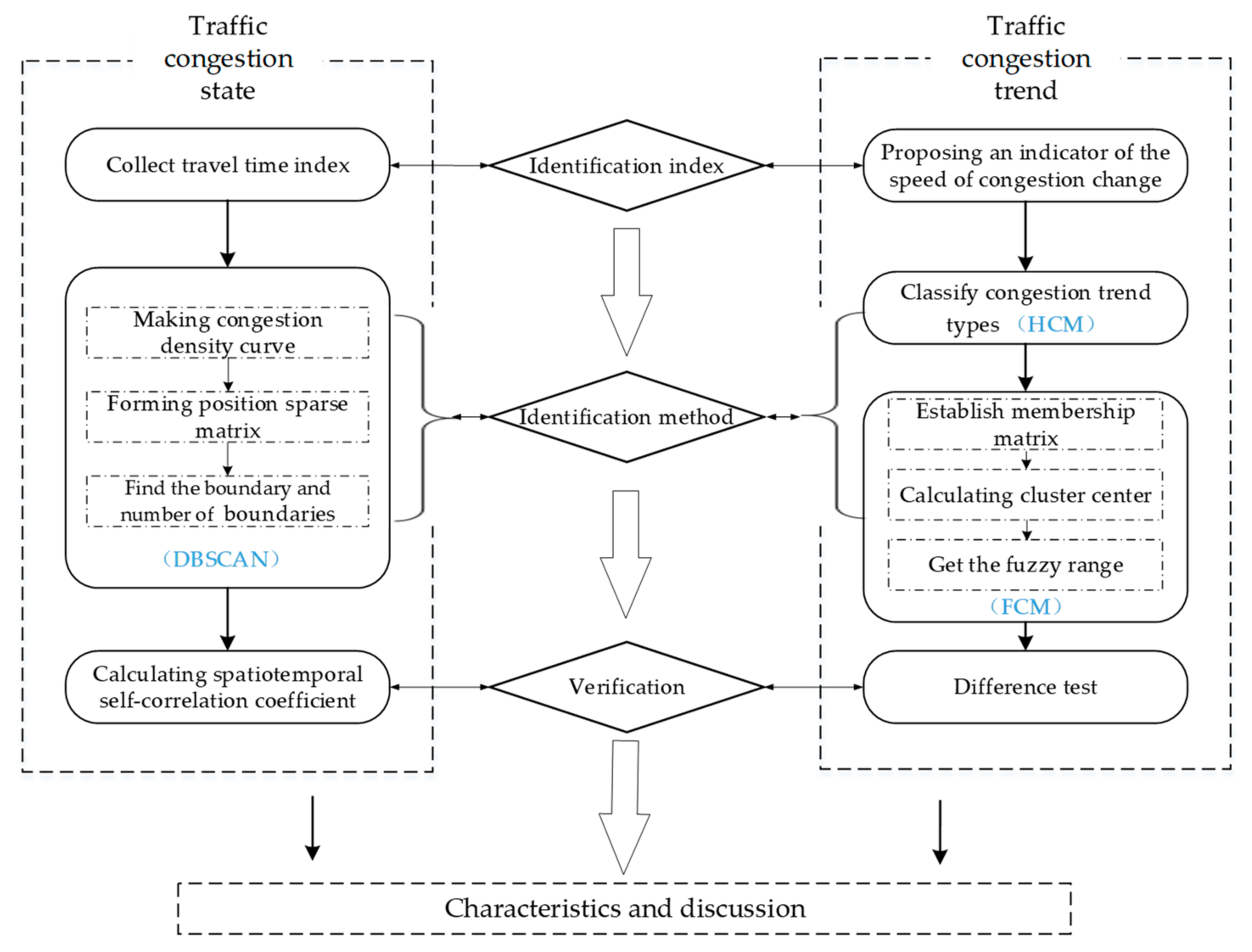
2.3. Methodologies
2.3.1. Identification Method of Traffic Congestion State of the Main Road in Cold-Climate Cities
2.3.2. Identification Method of Traffic Congestion Trend of the Main Road in Cold-Climate Cities
2.3.3. Effectiveness Verification Method
- Effectiveness Verification Method of Traffic Congestion State
- 2.
- Effectiveness Verification Method of Traffic Congestion Trend
3. Results
3.1. Identification Standard
3.1.1. Identification Standard of Traffic Congestion State
3.1.2. Identification Standard of Traffic Congestion Trend
3.2. Verification Results
3.2.1. Verification Results of Traffic Congestion State
3.2.2. Verification Results of Traffic Congestion Trend
3.3. Traffic Congestion Situation Characteristics of the Main Road in Cold-Climate Cities
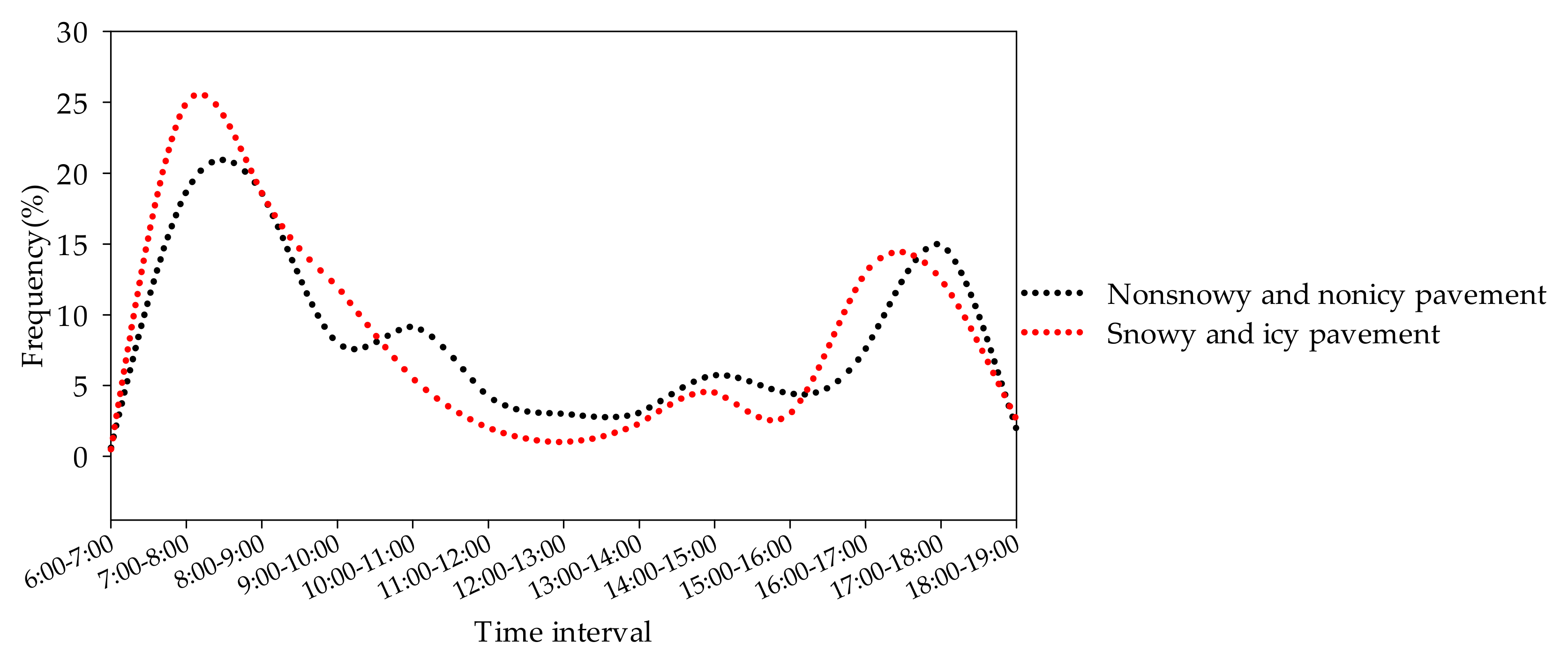
3.3.1. Temporal Characteristics
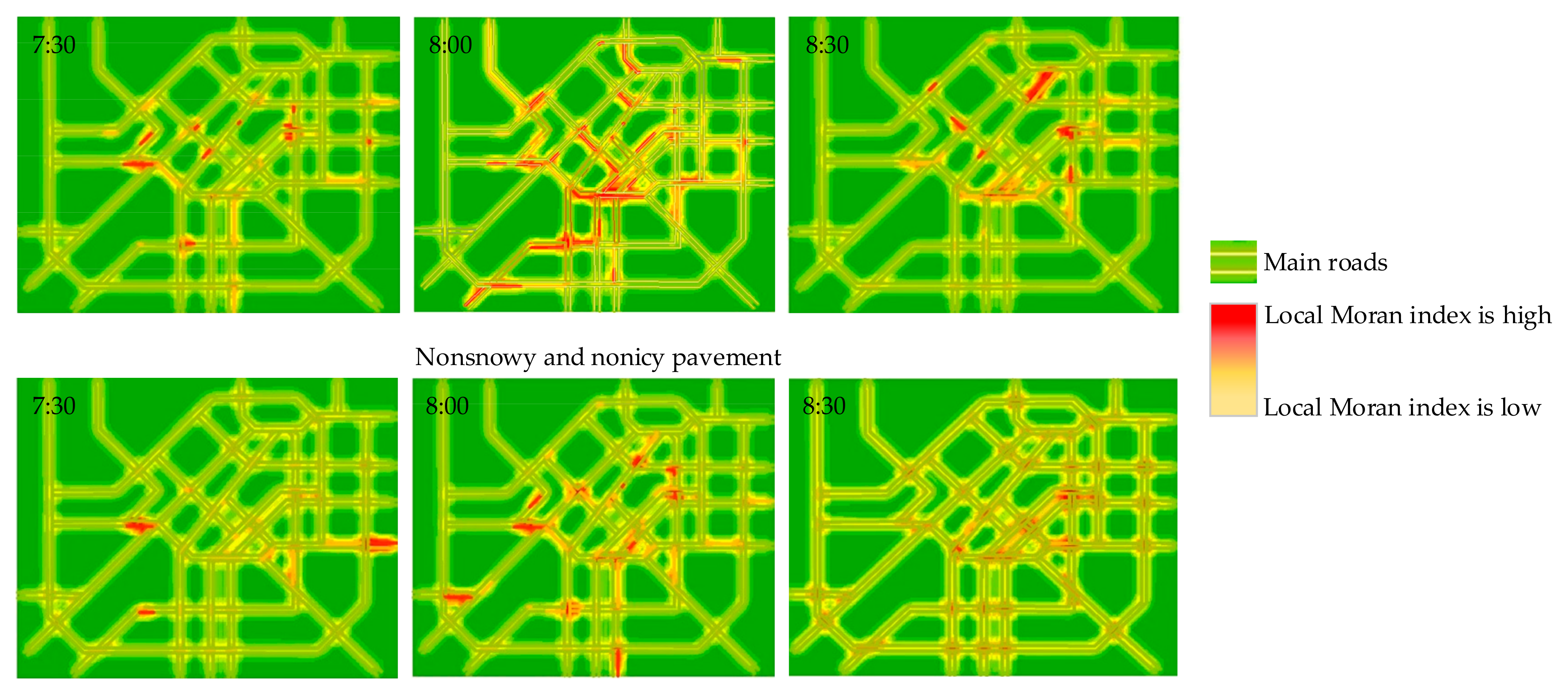
3.3.2. Spatial Characteristics
4. Discussion
5. Conclusions
Author Contributions
Funding
Institutional Review Board Statement
Informed Consent Statement
Data Availability Statement
Conflicts of Interest
References
- Graham, C.; Bob, P. INRIX Global Traffic Scorecard; Technical Report; INRIX: Kirkland, WA, USA, 2020. [Google Scholar]
- Qing, Y. The Market Circle of Beijing should be in the Fifth Ring Road. City House 2013, 10, 28–29. [Google Scholar]
- Aloi, A.; Alonso, B.; Benavente, J.; Cordera, R.; Echániz, E.; González, F.; Ladisa, C.; Lezama-Romanelli, R.; López-Parra, Á.; Mazzei, V.; et al. Effects of the COVID-19 Lockdown on Urban Mobility: Empirical Evidence from the City of Santander (Spain). Sustainability 2020, 12, 3870. [Google Scholar] [CrossRef]
- Kurek, A.; Macioszek, E. Extracting Road Traffic Volume in the City Before and During COVID-19 through Video Remote Sensing. Remote Sens. 2021, 13, 2329. [Google Scholar]
- Ku, D.G.; Um, J.S.; Byon, Y.J.; Kim, J.Y.; Lee, S.J. Changes in Passengers’ Travel Behavior Due to COVID-19. Sustainability 2021, 13, 7974. [Google Scholar] [CrossRef]
- Thermal Design Code for Civil Buildings, GB 50176–2016. Available online: http://www.mohurd.gov.cn/wjfb/201702/t20170213_230579.html (accessed on 30 August 2021).
- Baiyu, Z.; Fei, Z.; Jiang, Z. Analysis of the Interannual Variations and Influencing Factors of Wind Speed Anomalies over the Beijing–Tianjin–Hebei Region. Atmos. Ocean. Sci. Lett. 2017, 10, 312–318. [Google Scholar]
- Hou, T.; Mahmassani, H.; Alfelor, R.; Kim, J.; Saberi, M. Calibration of Traffic Flow Models Under Adverse Weather and Application in Mesoscopic Network Simulation. Trans. Res. Rec. J. Trans. Res. Board 2016, 2391, 92–104. [Google Scholar] [CrossRef] [Green Version]
- Maze, T.H.; Hans, Z.; Agarwal, M.; Burchett, G.D. Weather Impacts on Traffic Safety and Operations. J. Comp. Appl. 2006, 38, 455–459. [Google Scholar]
- Amiri, M.; Sadeghpour, F. Cycling Characteristics in Cities with Cold Weather. Sustain. Cities. Soc. 2015, 14, 397–403. [Google Scholar] [CrossRef]
- Thomas, N.; Luis, F.M.M. The Effect of Weather on the Use of North American Bicycle Facilities: A Multi-city Analysis Using Automatic Count. Transp. Res. A-Pol. 2014, 66, 213–225. [Google Scholar]
- Chi, L.B.; Zhou, L.F. Urban Residents Travel Mode Selection Rule during Period of Ice and Snow in Cold Region. J. Chang. Inst. Technol. 2019, 20, 112–118. [Google Scholar]
- Johannes, A.; Henk, J.Z.; Bernhard, H. Calibrating VISSIM to Adverse Weather Conditions. In Proceedings of the 2nd International Conference on Models and Technologies for Intelligent Transportation Systems, Leuven, Belgium, 22–24 June 2011. [Google Scholar]
- Solove, V.; Kuchinskaya, E.; Antonov, N.; Volotskiy, T. Analyzing Efficiency of Different Snow Removal Strategies in Terms of the System Wide Time Savings Using Dynamic Link Capacity in Large-Scale Microsimulation. Proc. Comp. Sci. 2020, 178, 116–124. [Google Scholar] [CrossRef]
- Macioszek, E.; Iwanowicz, D. A Back-of-Queue Model of A Signal-Controlled Intersection Approach Developed Based on Analysis of Vehicle Driver Behavior. Energies 2021, 14, 1204. [Google Scholar] [CrossRef]
- Pan, B.; Liu, S.; Xie, Z.; Shao, Y.; Li, X.; Ge, R. Evaluating Operational Features of Three Unconventional Intersections Under Heavy Traffic Based on Critic Method. Sustainability 2021, 13, 4098. [Google Scholar] [CrossRef]
- Li, C.; Yue, W.; Mao, G.; Xu, Z. Congestion Propagation Based Bottleneck Identification in Urban Road Networks. IEEE Trans. Veh. Technol. 2020, 69, 4827–4841. [Google Scholar] [CrossRef]
- Chaoyun, W.; Maobin, H.; Rui, J.; Qingyi, H. Effects of Road Network Structure on the Performance of Urban Traffic Systems. Phys. A 2021, 563, 1–10. [Google Scholar]
- Liangliang, C.; Rongrong, L.; Aizeng, L. Simulation of Traffic Microcirculation Optimization in Residential Area. J. Phys. Conf. Ser. 2021, 1972, 012109. [Google Scholar] [CrossRef]
- General, W. Main Roads Projects to Address Traffic Congestion; Office of the Auditor General Western Australia: Perth, Australia, 2015.
- Ruo, J.; Shenghong, D.; Ni, H.; Shuiying, L.; Zhiyuan, L. Literature Review on Traffic Congestion Identification Methods. J. South China Univ. Technol. 2021, 49, 124–139. [Google Scholar]
- Wei, D.; Junli, L. Identification Recurring and Incident Congestion on Freeways. J. Southeast Univ. 1994, 24, 60–65. [Google Scholar]
- Sánchez, G.S.; Bedoya, M.F.; Calatayud, A. Understanding the Effect of Traffic Congestion on Accidents Using Big Data. Sustainability 2021, 13, 7500. [Google Scholar] [CrossRef]
- Shi, Q.; Abdel, A.M. Big Data Applications in Real-Time Traffic Operation and Safety Monitoring and Improvement on Urban Expressways. Transp. Res. Part C Emerg. Technol. 2015, 58, 380–394. [Google Scholar] [CrossRef]
- Watanabe, S. Traffic Engineering; People’s Communications Press: Beijing, China, 1980; pp. 145–147. [Google Scholar]
- Description of Road Traffic Information Service Traffic Condition, GB/T 29107–2012. Available online: http://www.jianbiaoku.com/webarbs/book/71352/1430458.shtml (accessed on 30 August 2021).
- Transportation Research Board, American Road Capacity Manual(HCM2000). Available online: https://www.docin.com/p-1621684466.html (accessed on 30 August 2021).
- Transportation Research Board, American Road Capacity Manual(HCM2016). Available online: https://www.docin.com/p-1855934002.html (accessed on 30 August 2021).
- Tengfei, Z. Transportation Infrastructure and Urban Economic Development: Theoretical Mechanism and Empirical Research. Ph.D. Thesis, Hunan University, Changsha, China, 2019. [Google Scholar]
- Texas A&M Transportation Institute. Texas A&M University System; Urban Mobility Report; Texas A&M Transportation Institute: College Station, TX, USA, 2021. [Google Scholar]
- AutoNavi Map. Traffic Analysis Report of Major Cities in China; AutoNavi Map: Beijing, China, 2017. [Google Scholar]
- Evaluation Index System of Urban Road Traffic State Index, DB31/T 997–2016. Available online: http://www.jianbiaoku.com/webarbs/book/144923/4198840.shtml (accessed on 30 August 2021).
- Buisson, C.; Ladie, R.C. Exploring the Impact of Homogeneity of Traffic Measurements on the Existence of Macroscopic Fundamental Diagrams. Transp. Res. Rec. 2009, 2124, 127–136. [Google Scholar] [CrossRef]
- Xiao, Z.; Yuchuan, D.; Maoqiang, D. Study on Traffic Characteristics and Evaluation Method of Urban Trunk Road Based on Two Stream Theory. J. Transp. Inf. Saf. 2005, 23, 4–7. [Google Scholar]
- Emmanuel, K.; Ren, M.; Thobias, S. Bayesian Regression Approach to Estimate Speed Threshold under Uncertainty for Traffic Breakdown Event Identification. J. Transp. Eng. A-Syst. 2019, 145, 1–11. [Google Scholar]
- Sakib, M.K.; Kakan, C.D.; Mashrur, C. Real-Time Traffic State Estimation with Connected Vehicles. IEEE Trans. Intell. Transp. Syst. 2017, 18, 1687–1699. [Google Scholar]
- Enjat, M.M.D.; Widyantoro, D.; Rinaldi, M. A New Method for Analyzing Congestion Levels Based on Road Density and Vehicle Speed. J. Theo. Appl. Inf. Technol. 2017, 95, 6454–6471. [Google Scholar]
- Yuta, S. Lane Change Model of Vehicles Based on a Hybrid System Approach. In Proceedings of the 56th Annual Conference of the Society of Instrument and Control Engineers of Japan, Kanazawa, Japan, 19–22 September 2017. [Google Scholar]
- Nguyena, T.T.; Panchamy, K.; Simeon, C.; Calverta, H.L.; Vub, H.L. Feature Extraction and Clustering Analysis of Highway Congestion. Trans. Res. Part C 2019, 100, 238–258. [Google Scholar] [CrossRef]
- Mohanty, A.; Mahapatra, S.; Bhanja, U. Traffic Congestion Detection in A City Using Clustering Techniques in Vanets. Indonesian J. Elec. Eng. Comp. Sci. 2019, 13, 884–891. [Google Scholar] [CrossRef]
- Mondal, M.A.; Rehena, Z. Identifying Traffic Congestion Pattern using K-means Clustering Technique. In Proceedings of the 4th International Conference on Internet of Things: Smart Innovation and Usages, Bhimtal, India, 23–24 February 2018. [Google Scholar]
- Rong, G.; Yu, C. A Study on Polycentric Spatial Structure of Harbin. Planners 2020, 36, 5–11. [Google Scholar]
- Vachan, B.R.; Mishra, S. A User Monitoring Road Traffic Information Collection Using SUMO and Scheme for Road Surveillance with Deep Mind Analytics and Human Behavior Tracking. In Proceedings of the IEEE 4th International Conference on Cloud Computing and Big Data Analysis, Chengdu, China, 12–15 April 2019. [Google Scholar]
- Zhou, J.; Philip Chen, C.L.; Chen, L.; Wei, Z. A User-Customizable Urban Traffic Information Collection Method Based on Wireless Sensor Networks. IEEE T. Intell. Transp. 2013, 14, 1119–1128. [Google Scholar] [CrossRef]
- Levinson, H.S.; Lomax, T.J. A Travel Time Based Index for Evaluating Congestion. In Proceedings of the 66th ITE Annual Meeting, Minneapolis, MN, USA, 15–18 September 1996. [Google Scholar]
- Turner, S.; Margiotta, R.; Lomax, T. Monitoring Urban Freeways in 2003: Current Conditions and Trends from Archived Operations Data; Federal Highway Administration: Washington, DC, USA, 2004. [Google Scholar]
- Xiangfu, K.; Jiawen, Y.; Zhongyu, Y. Measuring Traffic Congestion with Taxi GPS Data and Travel Time Index. In Proceedings of the 15th COTA International Conference of Transportation Professionals, Beijing, China, 24–27 July 2015. [Google Scholar]
- Yun, Z.; Jianyu, W.; Jingting, J. Research on Urban Road Congestion Evaluation Based on TTI Method. In Proceedings of the 2017 World Transportation Conference, Beijing, China, 3–6 June 2017. [Google Scholar]
- Peng, Z.; Yingying, Z.; Fangshu, L.; Guangyu, Z.; Jifu, G.; Yongshen, Q. Dynamic Traffic Flow–Dispersion Model Based on TTI of Floating Cars. J. Transp. Eng. A-Syst. 2017, 143, 1–7. [Google Scholar]
- Ellis, D.; Lomax, T. The Cost of Congestion: TTI Leads Effort for the Governor’s Business Council. Texas Transp. Res. 2003, 39, 1–5. [Google Scholar]
- Saberi, M.; Bertini, R.L.; Bigazzi, A. Examining Segment Level Analysis of Travel Time Reliability Using Archived ITS Data. ResearchGate. Available online: https://www.researchgate.net/publication/266220861_Examining_Segment_Level_Analysis_of_Travel_Time_Reliability_Using_Archived_ITS_Data (accessed on 30 August 2021).
- Peng, Z.; Xiaosong, Z.; Fangshu, L.; Guangyu, Z.; Jifu, G. Road Congestion Probability Estimation Method and Its Application in Urban Traffic Operation Evaluation. Transp. Sys. Eng. Inf. 2015, 15, 161–169. [Google Scholar]
- Takemoto, A.; Munehiro, K.; Kasai, S. Experiment of Driving Behavior at Roundabout on Snow and Ice Pavement. Infrast. Plann. Rev. 2011, 67, 689–696. [Google Scholar]
- Yi, C. Study on Traffic State Probability Model of Urban Trunk Road under Ice and Snow Conditions. Ph.D. Thesis, Harbin Institute of Technology, Harbin, China, 2019. [Google Scholar]
- Gaur, M.K.; Goyal, R.K.; Raghuvanshi, M.S.; Bhatt, R.K.; Pandian, M.; Mishra, A. Geospatially Extracting Snow and Ice Cover Distribution in the Cold Arid Zone of India. Intern. J. Sys. Assur. Eng. Manag. 2020, 11, 84–99. [Google Scholar] [CrossRef]
- Yao, Y.; Xiaonan, G. Weather Cause Analysis and Forecast Index of Urban Ice and Snow Pavement. Meteor. Disa. Prev. 2016, 23, 29–32. [Google Scholar]
- Tang, W. Foreign Distinctive Methods of Fighting Snowstorm. Life Disa. 2011, 19, 10–14. [Google Scholar]
- Pilli, S.E.; Aapaoja, A.; Levikangas, P.; Kinnunen, T.; Hautala, R.; Takahashi, N. Evolving Winter Road Maintenance Ecosystems in Finland and Hokkaido, Japan. Intell. Transp. Sys. IET 2015, 9, 633–638. [Google Scholar] [CrossRef]
- Zha, K. Research on Trip Characteristics of Urban Residents during Winter in Cold Region. Master’s Thesis, Dalian Technology University, Dalian, China, 2017. [Google Scholar]
- Shearston, J.A.; Martinez, M.E.; Nunez, Y.; Hilpert, M. Social-Distancing Fatigue: Evidence from Real-Time Crowd-Sourced Traffic Data. Sci. Total Environ. 2021, 792, 148336. [Google Scholar] [CrossRef]
- Erhardt, G.D.; Roy, S.; Cooper, D.; Sana, B.; Castiglione, J. Do Transportation Network Companies Decrease or Increase Congestion? Sci. Adv. 2019, 5, 1–11. [Google Scholar] [CrossRef] [Green Version]
- Zhao, P.; Hu, H. Geographical Patterns of Traffic Congestion in Growing Megacities: Big Data Analytics from Beijing. Cities 2019, 92, 164–174. [Google Scholar] [CrossRef]
- Busari, A.A.; Loto, R.T.; Ajayi, S.O.; Odunlami, O.; Folake, A.; Kehinde, O. Ameliorating Urban Traffic Congestion for Sustainable Transportation. IOP Conf. Ser. Mater. Sci. Eng. 2021, 1107, 1–10. [Google Scholar] [CrossRef]
- Devi, S.V.; Wahab, H.A.; Gowtham, S.; Gowtham, G. Analyzing the Parking Demand Characteristics in Cultural Activity-Oriented City. IOP Conf. Ser. Mater. Sci. Eng. 2021, 1145, 1–10. [Google Scholar]
- Kohan, M.; Ale, J.M. Discovering Traffic Congestion through Traffic Flow Patterns Generated by Moving Object Trajectories. Comp. Environ. Urban Sys. 2019, 80, 101426. [Google Scholar] [CrossRef]
- Tsuboi, T.; Yoshikawa, N. Traffic Flow Analysis in Ahmedabad (India). Case Stud. Transp. Policy 2019, 8, 215–228. [Google Scholar] [CrossRef]
- Mena, Y.R.; Casas, J.; Gavalda, R. Probabilistic Model for Robust Traffic State Identification in Urban Networks. In Proceedings of the 2019 IEEE Intelligent Transportation Systems Conference, Auckland, New Zealand, 27–30 October 2019. [Google Scholar]
- Wei, Z. Stock Market Theories and Stock Price Behavior. J. Anhui Univ. 2002, 26, 40–45. [Google Scholar]
- Oğuz, R.F.; Uygun, Y.; Aktaş, M.S.; Aykurt, I. On the Use of Technical Analysis Indicators for Stock Market Price Movement Direction Prediction. In Proceedings of the 27th Signal Processing and Communications Applications Conference, Malatya, Turkey, 2–5 May 2018. [Google Scholar]
- Diep, H.T.; Desgranges, G. Dynamics of the Price Behavior in Stock Market: A Statistical Physics Approach. Phys. A Stat. Mech. Appl. 2019, 570, 125813. [Google Scholar] [CrossRef]
- Zhao, J.; Zeng, D.; Liang, S.; Kang, H.; Liu, Q. Prediction Model for Stock Price Trend Based on Recurrent Neural Network. J. Amb. Inetl. Hum. Comp. 2020, 1, 745–753. [Google Scholar] [CrossRef]
- Tse, C.K.; Liu, J.; Lau, C.M.; He, K. Observing Stock Market Fluctuation in Networks of Stocks. In Proceedings of the 1st International Conference on Complex Sciences, Shanghai, China, 23–25 February 2009. [Google Scholar]
- Saisai, J.; Dongyi, L.; Yaqi, Y. Research on Taxi Operation Characteristics by Improved DBSCAN Density Clustering Algorithm and K-means Clustering Algorithm. J. Phys. Conf. Ser. 2021, 1952, 042103. [Google Scholar]
- Malzer, C.; Baum, M. Constraint-Based Hierarchical Cluster Selection in Automotive Radar Data. Sensors 2021, 21, 3410. [Google Scholar] [CrossRef]
- Kellner, D.; Klappstein, J.; Dietmayer, K. Grid-Based DBSCAN for Clustering Extended Objects in Radar Data. In Proceedings of the 2012 IEEE Intelligent Vehicles Symposium, Madrid, Spain, 3–7 June 2012. [Google Scholar]
- Kaixin, Z.; Yaping, D.; Zhiyang, J.; Ji, Y. General Fuzzy C-means Clustering Algorithm Using Minkowski metric. Signal Process. 2021, 188, 108161. [Google Scholar]
- Ashokan, L.A.; Aju, C.D.; Vipin, S. Spatio-Temporal Analysis of Road Accident Incidents and Delineation of Hotspots Using Geospatial Tools in Thrissur District, Kerala, India. KN-J. Cartog. Geogr. Inf. 2019, 69, 255–265. [Google Scholar]
- Dapeng, G. Impacts of Rainfalls and Snowfalls on Urban Roads Traffic Performance. Master’s Thesis, Beijing Jiaotong University, Beijing, China, 2016. [Google Scholar]
- Yuxin, X. Jam Evaluation and Short-term Forecasting of Urban Expressway based on Weather—A Case Study in Xi’an City. Master’s Thesis, Chang’an University, Xi’an, China, 2017. [Google Scholar]
- Feifei, H. Study on the Influence Rules of Severe Weather on Traffic State of Urban Expressway Networks. Master’s Thesis, Beijing Jiaotong University, Beijing, China, 2016. [Google Scholar]
- Cambridge Systematics, Inc. Traffic Congestion and Reliability: Linking Solutions to Problems; Cambridge Systematics, Inc.: Medford, MA, USA, 2004. [Google Scholar]


| Annual Coldest Monthly Average Temperature (°C) | OR | Days with Daily Average Temperature Below 5 °C (D) | |
| Severe cold areas | (−∞, −10] | [145, +∞) | |
| Cold areas | (−10, 0) | (90, 145) |
| Indicator | Calculation Formula | Source | Identification Standard |
|---|---|---|---|
| Speed | — | Japan Highway Public Corporation [25] | When the speed is lower than 40 km/h, it is identified as congestion |
| China Standardization Administration «Road traffic information service traffic condition description» (GB/T 29107-2012) [26] | For main roads, when the speed range is (+∞, 30 km/h), it is unblocked, (15 km/h, 30 km/h] is slow, and (−∞, 15 km/h] is congestion | ||
| Road service level | — | American Road Capacity Manual (HCM2000) [27] | When the road service level reaches F level (the actual speed is 1/3~1/4 of the free-flow speed, and the traffic volume may exceed the road capacity), it is identified as congestion |
| American Road Capacity Manual (HCM2016) [28] | When the road service level reaches F level (when the free-flow speed is 55 km/h, the actual speed is ≤17 km/h, or the free-flow speed is 50 km/h, the actual speed is ≤15 km/h, and the volume capacity ratio is ≤1), it is identified as congestion | ||
| Occupancy | Chicago Transit Authority [29] | When the occupancy rate >30%, and the duration exceeds 5 min, it is identified as congested | |
| Travel Time Index (TTI) | American «Urban Mobility Report» [30] | No congestion level set | |
| AutoNavi Map [31] | (0, 1.5] is unblocked, (1.5, 1.8] is slow, (1.8, 2] is congestion, (2, 10] is very congestion | ||
| Traffic State Index (TSI) | China Standardization Administration «Evaluation index system for urban road traffic state» (DB31/T 997-2016) [32] | [0, 30] is unblocked, (30, 50] is relatively unblocked, (50, 70] is congestion, (70, 100] is severe congestion | |
| Degree of Congestion (DC) | Japan Highway Public Corporation [25] | Taking 12 h as an example, [0, 1) is congestion, [1, 1.75) is gradual congestion, and [1.75, +∞) is chronic congestion | |
| Inrix Congestion Index (ICI) | INRIX [1] | No congestion level set |
| January | February | March | April | May | June | |
|---|---|---|---|---|---|---|
| Average temperature (°C) | −16.9 | −11.9 | −1.3 | 8.6 | 15.8 | 20.6 |
| Precipitation (mL) | 3.1 | 6.1 | 8.1 | 12.7 | 67.3 | 129.7 |
| Precipitation days (D) | 5.8 | 5.7 | 5.7 | 6.7 | 10.3 | 13.5 |
| July | August | September | October | November | December | |
| Average temperature (°C) | 24.2 | 22.0 | 16.1 | 6.8 | −5.5 | −14.6 |
| Precipitation (mL) | 96.2 | 127.3 | 55.7 | 15.0 | 13.5 | 8.9 |
| Precipitation days (D) | 14.2 | 12.3 | 9.9 | 7.1 | 6.0 | 7.2 |
| Rain or Sleet | Snow | |
|---|---|---|
| Daytime temperature | ≤−3 °C | ≤−3 °C |
| Night temperature | ≤−3 °C | ≤0 °C |
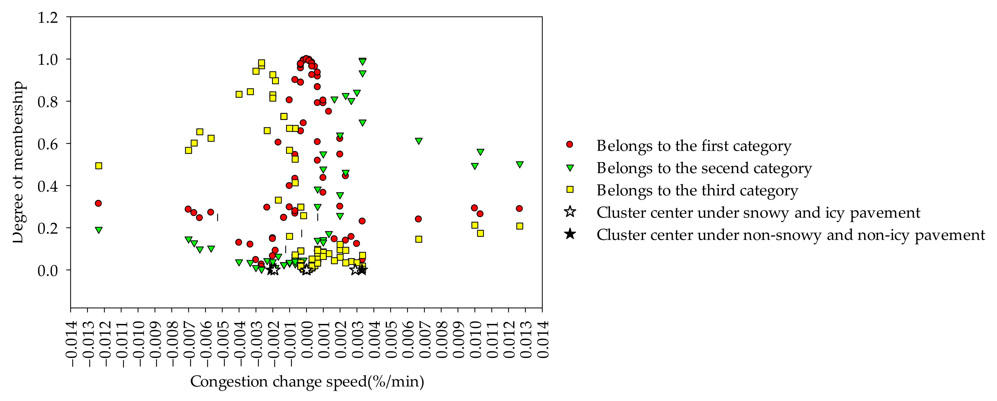
| Aggravating Type | Alleviating Type | Stable Type | |
|---|---|---|---|
| Non-snowy and non-icy pavement | (0.001, +∞) | (−∞, −0.001) | [−0.001, 0.001] |
| Snowy and icy pavement | (0.002, +∞) | (−∞, −0.002) | [−0.002, 0.002] |
| Variable | Sum of Deviationsquares | df | Mean Square | F | Significance | |
|---|---|---|---|---|---|---|
| Under the condition of non-snowy and non-icy pavement Speed of congestion change | Interblock | 0.000 | 2 | 0.000 | 65.048 | 0.000 |
| Intraclass | 0.000 | 85 | 0.000 | |||
| Total | 0.001 | 88 | ||||
| Under the condition of snowy and icy pavement Speed of congestion change | Interblock | 0.001 | 2 | 0.000 | 126.314 | 0.000 |
| Intraclass | 0.000 | 89 | 0.000 | |||
| Total | 0.001 | 92 | ||||
Publisher’s Note: MDPI stays neutral with regard to jurisdictional claims in published maps and institutional affiliations. |
© 2021 by the authors. Licensee MDPI, Basel, Switzerland. This article is an open access article distributed under the terms and conditions of the Creative Commons Attribution (CC BY) license (https://creativecommons.org/licenses/by/4.0/).
Share and Cite
Pei, Y.; Cai, X.; Li, J.; Song, K.; Liu, R. Method for Identifying the Traffic Congestion Situation of the Main Road in Cold-Climate Cities Based on the Clustering Analysis Algorithm. Sustainability 2021, 13, 9741. https://doi.org/10.3390/su13179741
Pei Y, Cai X, Li J, Song K, Liu R. Method for Identifying the Traffic Congestion Situation of the Main Road in Cold-Climate Cities Based on the Clustering Analysis Algorithm. Sustainability. 2021; 13(17):9741. https://doi.org/10.3390/su13179741
Chicago/Turabian StylePei, Yulong, Xiaoxi Cai, Jie Li, Keke Song, and Rui Liu. 2021. "Method for Identifying the Traffic Congestion Situation of the Main Road in Cold-Climate Cities Based on the Clustering Analysis Algorithm" Sustainability 13, no. 17: 9741. https://doi.org/10.3390/su13179741
APA StylePei, Y., Cai, X., Li, J., Song, K., & Liu, R. (2021). Method for Identifying the Traffic Congestion Situation of the Main Road in Cold-Climate Cities Based on the Clustering Analysis Algorithm. Sustainability, 13(17), 9741. https://doi.org/10.3390/su13179741