Abstract
Tourism has direct and indirect implications for CO emissions. Therefore, it is necessary to develop tourism management based on sustainable tourism, mainly in the transport process. Tourist itinerary planning is a complex process that plays a crucial role in tourist management. This type of problem, called the tourist trip design problem, aims to build personalised itineraries. However, planning tends to be biased towards group travel with heterogeneous preferences. Additionally, much of the information needed for planning is vague and imprecise. In this paper, a new model for tourist route planning is developed to minimise CO emissions from transportation and generate an equitable profit for tourists. In addition, the model also plans group routes with heterogeneous preferences, selects transport modes, and addresses uncertainty from fuzzy optimisation. A set of numerical tests was carried out with theoretical and real-world instances. The experimentation develops different scenarios to compare the results obtained by the model and analyse the relationship between the objectives. The results demonstrate the influence of the objectives on the solutions, the direct and inverse relationships between objectives, and the fuzzy nature of the problem.
1. Introduction
The service sector plays a major role in the world economy [1], and it represented 65% of worldwide gross domestic product (GDP) in 2019, surpassing agriculture, industry, and manufacturing [2]. Tourism is included in the services sector, and is a heterogeneous sub-sector of the economy. This sub-sector is made up of different organisations that offer services associated with transportation, accommodation, attractions, and food, among others, to satisfy tourists [3]. Tourism has grown and is now established as a solid alternative for economic development [4]. However, the pandemic generated by the SARS-CoV-2 coronavirus stopped tourism activities around the world, producing a negative impact on the world economy [5]. Nevertheless, there have also been some positive impacts that emerged on the environment which favours tourism [6,7]. The cumulative positive and negative effects of the pandemic have given rise to opportunities to rethink and strengthen tourism [8,9]. These opportunities can be framed in the direct and indirect contribution that tourism has played while meeting Sustainable Development Goals (SDGs) through sustainable tourism [10,11]. In addition, sustainable tourism can benefit partner organisations in terms of increased consumption, tourist arrivals, brand equity, opportunities to reach other market segments, among other direct and indirect benefits [12,13].
One of the global and latent problems for tourism is climate change [14]. Tourism is very sensitive to climate change, and it is also one of the sectors with the highest contribution of CO emissions to the environment [15]. The growing interest in the relationship between tourism and climate change is not evident in the literature [14,16]. Tourism management must face climate change, and research focused on carbon emissions must be developed [17]. The transport activity that is associated with tourism is relevant in terms of CO emissions [18]. Emissions from transport have been widely studied in the literature, although without any link to tourism [19]. Transport is an intrinsic part of the realisation of tourist itineraries and, therefore, of tourist planning. These activities ensure the mobility of tourists to the tourist destination and between their points of interest (POIs), even determining their attraction [20,21].
Tourism management includes travel itinerary planning processes, which are complex problems [22]. In the literature, this problem is called the tourist trip design problem (TTDP) and is generally modelled as an orienteering problem (OP) or a team orienteering problem (TOP) [23,24]. The TTDP aims to design a travel itinerary for tourists maximising their benefits without exceeding a budget [25]. Itinerary planning can include transportation, visiting hours, budget, and maximum duration of the trip [26,27,28]. Planning for groups can consider the preferences of each of the tourists (i.e., within a group of tourists, each one may have different preferences on each specific POIs). This type of variant is called heterogeneous preferences [29]. The results of group planning should not favour one tourist above the others. Therefore, benefits must be equitable [30]. Equity is approached from the social dimension as one of the three dimensions of sustainability based on the triple bottom line (TBL) [31,32,33]. There are limited works on the social dimension in routing problems in operations research due to the complexity of its measurement [34]. It is necessary to include all three dimensions (economic, social, and environmental) when defining sustainability in tourism management and itinerary planning. In this work, the equity of the group benefit is included to minimise the differences between the benefits obtained by each tourist in the itinerary. The tourism planning process is complex and sensitive to the data available from the real world. This process requires up-to-date and available information [35]. Therefore, public and private sector organisations that make up the tourism supply chain [36], must adopt clear policies for the articulation and provision of information.
Additionally, in practice, there is a certain degree of uncertainty in these data; this is incomplete and imprecise data. Nevertheless, information is not the only element which is vague and ambiguous; the criteria and restrictions defined by the decision-makers are also vague and ambiguous, and in many cases the natural way to express them is with the use of a linguistic term [24,37,38]. Linguistic variables describe imprecise and subjective information from human judgment such as preference ratings [39,40]. This type of component of planning problems can be approached as fuzzy components [41,42] because it does not allow the construction of distributions under stochastic approaches [43].
This work proposes a new multi-objective model of mixed integer programming for the design of tourist itineraries. The model addresses the multi-route planning problem for a group of tourists with heterogeneous preferences and transport mode selection. It also accounts for CO emissions, equity, POI time windows, maximum and minimum tourist capacity on the route, and available budgets. Uncertainty is also considered in some components and approached in fuzzy terms. A set of tests with theoretical and real instances were conducted to verify the efficiency of the model. The main contributions are as follows:
- A model for group planning of sustainable tourism itineraries is presented and formulated, which articulates three objectives. These objectives are maximising the individual benefits of tourists (individual profit), maximisation of equity (equity in group profit), and minimising CO emissions derived from multi-modal transport. The problem modelled as TOP considers travel costs and budgets. Thus, all three dimensions of TBL are included;
- The social dimension is incorporated into the process of constructing itineraries under the concept of equity in the group profit. This dimension is measured based on the difference in personal benefits. The objective is to minimise the difference between the highest and lowest profit obtained by a tourist;
- The costs of CO emissions emitted by multi-modal transport in the itinerary are calculated. The only evidence of in the literature where this concept is applied is in [44];
- Uncertainty is considered in some of its components, and a fuzzy approximation is used to address it. Thus, fuzzy numbers are considered to quantify the heterogeneous preferences of tourists associated with the first and second objectives. Flexible (fuzzy) time window constraints, budget, and maximum travel time are also considered;
- The model also provides support for decision-making in tourism planning under COVID-19 scenarios. The maximum capacity of tourists on the route maintains the permissible occupancy at the sites of interest. This limitation helps to ensure the care and health of tourists.
Finally, such tools have a significant impact on the management process. It also supports the development of tourism self-management platforms and applications [45]. In this way, different actors in the chain can benefit by generating greater interest and perceived value of visitors to the area due to the facility of planning itineraries in the territory; the perceived value of a tourist destination suggests a relationship between the benefit obtained and the sacrifice associated with the complexity of planning [46,47].
The remainder of this document is structured as follows. Section 2 presents a review of the literature. Section 3 addresses and formulates the model with the different novel aspects. Section 4 describes the evaluation of the results of the experimentation using the designed model and certain instances. Finally, Section 5 summarises the conclusions.
2. Background
TTDP has been widely studied since its introduction in 2007 by Vansteenwegen and Van Oudheusden [23]. The most commonly used model to address this problem is TOP and its variants, such as TOP with time windows (TOPTW) [24]. Several variants of this model are used to incorporate realistic aspects of the problem, such as the use of temporal dependence, selection of transport modes, multiple periods, heterogeneous preferences, and uncertainty. Nevertheless, present day strategies for sustainable development and the need to offset climate change require sustainability aspects to be included in planning tourist routes. This review of the state of the art focuses on the TTDP models that consider CO emissions, heterogeneous preferences in tourist groups, and uncertainty addressed with a fuzzy approach.
2.1. Transport and CO Emissions
Infrastructure and transport within the tourist area are criteria for competitiveness in the sector [48]. Transport is a critical and dynamic process of tourism, which facilitates physical movement to points of interest [20]. Transportation is key to the interrelation between actors in the tourist chain and affects the accessibility to the tourist destination, the distance travelled, and the comfort of the trip [49,50]. Several variables affect the physical movement of goods and people (e.g., times, travel costs, delays, modes of transport, among others) [51]. Contextualised variables generate variants of transport models, among which are the so-called “green” variants. This type of variant seeks to minimise CO emissions considering fuel consumption and electrical energy by the vehicle [52,53,54].
In the TTDP, transportation facilitates the organisation of the movement and flow of people or goods [55]. The modelling includes the movement of a tourist from the origin to a POI, from a POI i to one j, or from a POI to the end node, travel time, mode of transport and emissions, among others aspects [56]. Transportation emits large amounts of CO, and CO emissions contribute to climate change [57]. To our knowledge, only Susanty et al. [44] addresses CO emissions from transport in the TTDP in the literature.
The literature is more numerous on models of TTDP that include transport, such as multimodal and time-dependent variants. Abbaspour and Samadzadeg [58] develop a genetic algorithm (GA) to solve the TTDP that includes multimodal transport and real traffic parameters and time constraints. Garcia et al. [59] integrate public transport in the construction of tourist routes. The problem is modelled as an OP with time and time-dependent windows (TDOPTW) and solved with a hybrid approach of two heuristics, the travel times are previously calculated, and then the route is constructed. Subsequently, Abbaspour and Samadzadegan [60] applied an evolutionary algorithm (EA) based on two AGs to solve the tour planning problem in time-dependent urban areas (the route depends on the start time). Garcia et al. [61] develop a personalised electronic tourist guide (PET) based on a time-dependent TOP with time windows (TDTOPTW) that includes public transport. The methodology to solve it uses a hybrid approach based on iterated local search (ILS). Gavalas et al. [55] develop the metaheuristics called time dependent CSCRoutes (TD_CSCR), time-dependent slack CSCRoutes (TD_SℓCSCR), and average travel times CSCRoutes (AvgCSCR). These algorithms are applied to solve the TDTOPTW considering the periodicity of the travel times. Gavalas et al. [62] develop a tool for the construction of tourist itineraries called eCOMPASS that considers the departure time and the mode of transport on the tourist route.
Wu et al. [63] develop a mathematical model that considers the selection of transport modes in each arc, the travel budget, and the maximum travel times. Yu et al. [64] addresses the multimodal variant to TOPTW (MM-TOPTW) to model the TTDP with transport mode selection. It uses the metaheuristic two-level particle swarm optimization with multiple social learning terms (2L-GLNPSO). Liao and Zheng [65] designs a model that considers the construction of itineraries in stochastic and time-dependent environments. The model is solved with a hybrid heuristic based on random simulation (RS-HA) that starts constructing random initial solutions and following applies an evolutionary hybrid that combines GA with a differential evolution algorithm (DEA). Zheng et al. [38] consider the complexity of urban tourism transport systems, congestion, and the transport needs of tourists for the design of a multi-objective model of one-day urban tourist routes with the selection of the transport mode (TTDP-TMC). The model is solved through a hybrid algorithm of a non-dominant ordering heuristic (NSHA), particle swarm enhanced optimisation (PSO), and DEA. Zhang et al. [66] develop a model for the construction of itineraries in scenic routes considering the modes of transport. Kargar and Lin [67] consider the possible environmental implications of tourist itineraries by creating groups of tourists that use a single mode of transportation (i.e., taxis). Ntakolia and Iakovidis [68] develop a mixed binary quadratic programming model (MIQPL) to solve the multiobjective TTDP considering modern transport modes. The model is solved through a swarm intelligence graph-based pathfinding algorithm (SIGPA). Finally, works have been developed that incorporate the use of electric vehicles (EV) for the generation of more environmentally friendly tourist itineraries, such as Wang et al. [69], Karbowska-Chilinska and Chociej [70], and Karbowska-Chilinska and Chociej [71].
2.2. Heterogeneous Preferences and Equity
The planning of tourist routes is generally oriented to the design of routes for a single tourist. However, tourist trips are in practice carried out in groups, and many tourists prefer it that way [29,67,72]. The planning of group tourist routes must consider the individual preferences of each tourist (i.e., if a tourist prefers to visit different POIs to another tourist from the same group). This type of TTDP variant is called TTDP with heterogeneous preferences [29], and some works are available in the literature. Malucelli et al. [73] develop an extension of the OP called multi-commodity orienteering problem with network design (MOP-ND) to model the route design problem for various cycle-tourists. The model considers the preferences of each tourist who incorporates different benefits on the same route. Sylejmani et al. [72] develop an extension of the TTDP called tourist group trips problem modelled as a multiple multi-constraint TOPTW (MCMTOPTW). The authors approach the problem in three different versions and develop three algorithms to solve them. The first is the single trip planner that designs the route for a single tourist according to his preferences. The second is the tourist group builder that groups tourists into clusters according to their preferences and social relationship. The third is a group trip planner that groups tourists based on multiple preferences. Zheng and Liao [29] develop an algorithm called non-dominated classification algorithm (NSACDE) that hybridises ant colony optimization (ACO) and DEA to solve a bi-objective TTDP model with heterogeneous preferences. Finally, Kargar and Lin [67] developed a route planning model that considers multiple days, urban tourism, POI categories, and heterogeneous preferences for a group of tourists that maximises profit and minimises travel time, distance, and cost.
The social dimension that is part of the TBL can be approached from different aspects. Sylejmani et al. [72] apply a social relationship index for the construction of routes that considers the proximity of tourists (degree of kinship or friendship) valued on a Likert scale to group them on the routes. Zheng and Liao [29] maximise the minimum profit obtained by a tourist to maintain a notion of equity in the group. Finally, Kargar and Lin [67] are committed to increasing the social welfare of tourists by jointly participating in urban tourism.
Equity, as a multidimensional concept of distribution of costs, benefits, participation, and recognition, is part of the social dimension and is defined in three dimensions: distribution equity, procedure equity, and recognition equity [30,74]. Distribution equity concerns the distribution of costs, responsibilities, rights, and benefits. Therefore, based on this concept, the route planning of a group of tourists must generate an equitable benefit (equity in group benefit). That is, a single tourist cannot be extremely rewarded or be taken advantage of with regards to other tourists in the final route planning.
2.3. Fuzzy Approach to TTDP
Tourism planning in real contexts is complex and full of uncertainty. The information available in many cases is imprecise and incomplete. For example, travel times are not available or are very difficult to specify due to traffic problems and congestion, or the exact expressions for which to describe the benefits, interests, and preferences offered by a POI are complex tasks for a tourist [37]. Stochastic and fuzzy approaches are usually used to describe the imprecise or uncertain parameters in real-world decision making and optimisation problems. Fuzzy sets and systems are used as methodologies when it is difficult for experts to provide a probability distribution due to the uncertainty or lack of knowledge of the data. On the contrary, if a distribution can be generated that represents the behaviour of the data, then the stochastic approach could be used [75]. Nevertheless, tourists in general almost always incompletely express the information necessary for planning with the available knowledge, and, as such, their preferences and their decision criteria are also expressed in an imprecise and vague way, instead using natural language which take on the role of linguistic variables [39]. Given these circumstances, it is necessary to address these optimisation problems with ambiguous and imprecise parameters and components expressed with linguistic variables, with fuzzy approaches, and generate solutions of the same nature without using exact calculations [76].
Few studies in the TTDP literature have applied the fuzzy approach and the stochastic approach. Stochastic and probabilistic methodologies include the works in [37,38,65,77,78]. Research using fuzzy optimisation to solve tourist route problems has been undertaken. Matsuda et al. [79] develop a fuzzy optimal routing problem for sightseeing (FORPS) that considers ambiguity and variation in travel times. Hasuike et al. [80] consider travel times and satisfaction generated by fuzzy activities. Hasuike et al. [81] apply time-expanded network (TEN) with fuzzy times and satisfaction value. Subsequently, Hasuike et al. [82] proposed, in addition to the uncertainty in travel times, the fatigue-dependence of tourist satisfaction. Brito et al. [24] consider the benefit of each POI as a fuzzy parameter, modelling the problem as a TOPTW and solve it with a fuzzy greedy randomised adaptive search procedures (FuzzyGRASP). Expósito et al. [83] and Expósito et al. [25] develop a TTDP with clustered POIs (TTDP-Clu) with the objective function and fuzzy constraints, which is then solved with a FuzzyGRASP.
3. Mathematical Modelling
3.1. Model Formulation
This section will formulate the fuzzy TOPTW model for a group of tourists with heterogeneous preferences and sustainability criteria. There are different modelling approaches for the TTDP, such as the optimal tourist problem (OTP), generalised maximum covering problem (GMCP), among others. However, TOPTW is an extension of TOP generally used to model the TTDP for several reasons. (i). There is a score or benefit associated with each POI, (ii). it is not mandatory to visit all POIs, (iii). each POI generally has an opening and closing time, (iv). there is a budget that limits the travel, and, finally, (v). the aim is to maximise the score collected [23,24].
Sustainability is approached from the environmental and social scopes. The environmental scopes considers the CO emissions produced by the chosen transport used on the routes. The social scope calculates the equity of the group profit. The model presents three objectives associated with the individual profit of the group members, the equity of the group profit, and the cost of CO emissions. The weighted sum method is used in the multi-objective function to convert it into a scalar function [84]. The method is efficient and easy to use. Additionally, it has been used in different optimisation problems for tourism planning and routing [68,85,86,87]. Therefore, to obtain an overall value for each solution of the model, it is calculated by summing the results of each objective multiplied by their respective weights [88]. In our model, we assigned the weights , , and .
The expected result builds different routes represented by a directed graph , where V is the set of vertices and A is the set of arcs . Routes are determined for groups of tourists, and in our model a group tourists can move in different modes of transport . Each POI i presents a time window that limits the visit, a visit time , and a score that represents a valuation of it. Additionally, each route has a maximum capacity and a minimum of tourists. Each tourist has a preference associated with the POIs, a maximum budget to invest in the route and a maximum time available for it. The time, cost, and emissions matrices are calculated through Equations (1)–(3), respectively.
The index, parameters, and variables of the model are described in the following Table 1 and Table 2.

Table 1.
Index and parameters.
Table 2.
Binaries and positives variables.
The formulation of the model is as follows:
Multi-objective function
Subject to
The objective function (4) maximises the individual profit of tourists, maximises the equity of the group profit, while minimising the distance between the maximum and minimum profit received by tourists. Additionally, it minimises CO emissions considering the number of tourists using public transportation and private transportation. Constraints (5) ensures that routes start and end at node . Constraints (6) ensures that each tourist belongs to only one route. Constraints (7) are flow constraints and ensure the continuity of the path. Constraints (8)–(10), ensure the maximum and minimum capacities in the routes, and activate the auxiliary variables. Constraints (11) ensure that a node belongs to only one path. Constraints (12) and (13) establish that in each arc, only one mode of transport must be used per tourist. Constraints (14) calculate the arrival time at each node. Constraints (15) and (16) calculate the travel time of each tourist and ensure that the maximum travel time is satisfied. Constraints (17) ensure that time windows limits are maintained. Constraints (18) ensure that tourists’ budget is not exceeded. Constraints (19) guarantees that all tourists are on the routes. Constraints (20) ensures the opening of the routes. Constraints (21) calculates the number of tourists who make an arc in a public transport mode. Constraints (22) determines the particular transport usage in the arc . Constraints (23) calculate the maximum and minimum profit for tourists. Finally, Constraints (24) and (25) define the nature of the variables. Note that the ∼ symbol denotes that the objective function is fuzzy. Similarly, the symbol f denotes that the constraints are fuzzy.
3.2. Fuzzy Optimization
This section describes the use of fuzzy optimisation approach in the model and how these techniques are applied to solve an optimisation problem with fuzzy components. In this methodology, fuzzy sets and systems solve decision and optimisation problems with uncertainty in some of the components and expressed in fuzzy terms. We are faced with a fuzzy optimisation problem, where the discussion about the solutions does not focus on the feasibility and optimality of the solutions but only on their degree of feasibility and optimality, that is, their linguistically expressed feasibility and optimality. Bellman and Zadeh [89] introduced the fundamentals of fuzzy optimisation problems, where goals and constraints can be defined and characterised as fuzzy sets using membership functions. This approach requires that the formulation and solutions of the problem be approached using fuzzy number representations and their operations.
In the previous section, we formulated the TOP as a LP problem with fuzzy coefficients in the objective function and fuzzy inequalities in some constraints. Fuzzy linear programming (FLP) constitutes the basis for solving fuzzy optimisation problems and their solution methods have been the subject of many studies in the fuzzy context. Different FLP models can be considered according to the elements that contain imprecise information that are used as a basis for the classification proposed in [90]. These models are: models with fuzzy constraints, models with fuzzy goals, models with fuzzy costs and models with fuzzy coefficients in the technological matrix and resources. In addition, a fifth model, the general fuzzy problem, in which all of the parameters are subject to fuzzy considerations, can be studied. The corresponding methodological approaches that provide solutions to FLP [91], provide methods for solving TOP with fuzzy terms. Therefore, this problem can be solved in a direct and simple way, obtaining solutions that are coherent with their fuzzy nature.
The methodology consists first in finding feasible solutions; i.e., solving the optimisation problem with fuzzy constraints, and secondly, solving the problem with fuzzy coefficients in the objective function.
Namely, Verdegay [90], using the representation theorem for fuzzy sets, proves that the solutions for the case of linear functions can be obtained from the auxiliary model:
where is the tolerance level vector. Thus, we use that approach to obtain an equivalent model to deal with fuzzy constraints. Applying the resulting model we obtain a range of solutions varying with . Therefore, the Constraints (15), (17), (18), and (23) are replaced by the new Constraints (27)–(30) for obtaining a new auxiliary model.
The next step is to deal with the fuzzy coefficients in the objective function. The fuzzy model is transformed into a simpler auxiliary model. The method proposed the use of an ordering function g that allows the comparison between fuzzy numbers, which facilitates maximisation of the objective function. Therefore, the objective function (4) is replaced by:
In our case, similarly to Kargar and Lin [67] and Ruiz-Meza and Montoya-Torres [92], tourists’preferences are obtained by multiplying a preference factor associated with each POI and the valuation of each POI. is a vector that takes values from 0 to 1. The smaller the values of this vector, the lower the tourist’s preference for a POI. However, when a tourist establishes his interest or preference in a real context, it is usually done in natural language in a vague and imprecise way, expressing it in terms of linguistic variables (for example at least 0.7, about 0.6). In these cases, we can consider the fuzzy preferences and express them as fuzzy numbers. We can represent these quantities as fuzzy triangular numbers whose membership function is one of the best known to represent fuzzy components in fuzzy optimisation problems [93]. Thus, the fuzzy number where , is a triangular number. This number is defined as a triplet of real numbers where . The membership function of these numbers is the following [79,94].
To obtain fuzzy triangular numbers that express tourist preferences, we use the information of the upper limits and lower (for example, between 0.6 and 0.9). The mean value is then calculated. As we described previously, according to the fuzzy components, different fuzzy models can be obtained and transformed to be solved [90]. In our model, the imprecision is in the objective and in the constraints. To evaluate the fuzzy objective function, a fuzzy number ordering function is used. To solve this problem we use the Adamo index or relation and a new auxiliary model is obtained . Subject to . Where y d is the right side margin that is obtained [95,96].
An application of the Adamo index to the first objective function which corresponds to the calculation of the profit results in Equation (33). and correspond to the tourist preference factors u for each POI i.
3.3. Consideration of CO Emissions
The CO emissions depend on the type of vehicle and its use (public or private transportation). According to Department for Business, Energy, and Industrial Strategy [97], CO emissions for public transport vehicles are calculated based on the number transported. Therefore, for buses, the average emissions are 0.10391 kgCO/passenger-km. In our model, the mode of transport and the use made of it by tourists are distinguished. The CO emissions in public transport are calculated according to the number of tourists who make the route of each arc on the route k (e.g., if the arc does it the tourists . The emission calculation is obtained by multiplying the emission rate by the number of tourists that make the trip).
For private vehicles, the calculation is based on the average emission of different private vehicles belonging to various market segments [97]. Emissions correspond to 0.18014 kg CO/km. However, for this work, the construction of a group itinerary is considered. One of the consumption factors in vehicles corresponds to the different occupancy rate [98,99]. Therefore, if the average occupancy established in five occupants is not exceeded, the CO emission rate in the arc remains the same for a number of tourists . The emission costs are calculated based on the costs per kg reported by European CO trading system [100] which corresponds to .
4. Experimentation
The model was coded in the general algebraic modeling systems (GAMS) optimisation software and solved through the CPLEX solver on a computer with the following references: 20 GB of RAM, an Intel Core CPU GHz, TB hard drive, and a 64-bit operating system. For the experimentation, two types of instances were used, some elaborated ad-hoc for the investigation and another real-world one, of medium and small size, respectively. In total, 300 tests were carried out for the instances used (288 for the hptoptw-j21 elaborated instance and 12 for the real-world Toptw-jMun-d instances). Both instances are available at https://jrmontoya.wordpress.com/research/instances/, accessed on 4 May 2021.
The instance hptoptw-j21a is made up of 21 nodes including the starting node (0). For the tests with this instance, variations of the weights associated with the objectives were made, as shown in Table 3. The weights , , and were set by the decision-maker. However, we do not use methods such as Diakoulaki [101], entropy [102], or simple ranking to establish fixed weighted values. The decision to establish the importance of each objective may vary according to the criteria of each tourist in a real situation. A wide margin of combinations is considered to increase the set of solutions obtained. The combinations of weights cover the increase and decrease in each objective by one decimal point at a time. In this way, the aim is to include as much variation in the weights as possible. In addition, the vector of weights includes the Utopia points to generate solutions considering only one objective (e.g., , , ).
Table 3.
Variations of the weights of the objectives. Each combination of weights adds up to a total of 1 (100 %).
Solutions were also obtained with the fuzzy model, . The values of , , and are . Finally, the value of was . All these values were established by the decision-maker. The time budgets for tourists correspond to , respectively. The cost budget for travel is 1000 for all tourists. The cost per km travelled according to the mode of transport used is . Finally, the maximum and minimum capacity of tourists per route is and , respectively. The time programmed for the execution of the model was 5400 s ( h or 90 min).
Full test results for all variations of , , , and are available at https://jrmontoya.wordpress.com/investigation/instances/, accessed on 10 July 2021.
In Figure 1, the objective comparison graph is shown. There is a directly proportional relationship between the objectives and that corresponds to the maximisation of the benefit of each tourist and the minimisation of the costs associated with the emissions of CO, respectively. Observe that when profit obtained increases so do emissions (see Figure 1a). This relation can be explained by the increased number of POIs visited on the route. However, it is necessary to consider the tourist’s preferences because a higher score does not necessarily mean more points of interest. The relationship between objectives and , preferences and participation in group profits also shows a direct relationship (see Figure 1d). The model tries to minimise objective and with a lower value, the smaller the difference of the benefits of the tourists in the group. In this scenario conflicts are generated between both objectives.
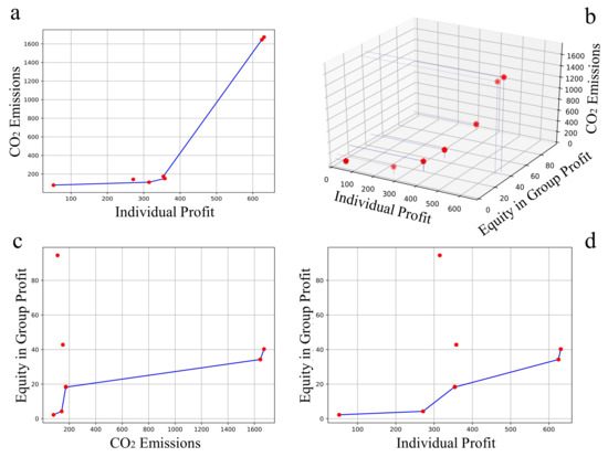
Figure 1.
Pareto frontier. Relationship between the objectives (hptoptw-j21a instance) comparing two by two (a,c,d), and a general one (b).
An example of the behaviour of the solutions according to the variation of , , , and is shown in Table 4 with , , and = .
Table 4.
Test hptoptw-j21a instance.
When observing the results of the experimentation, despite high computation times, no solutions with a gap of 0% were found. In real practical cases, route planning needs answers in shorter times. This high gap is consistent with the NP-hard nature of the problem. As the value of the -cuts decreases, an increase in the gap of the solutions is observed. This suggests that by relaxing the constraints the model is more complex to solve. On the other hand, varying diversifies the solutions for , and to a lesser extent in . Therefore, the variation of -cuts does not considerably affect the CO emissions. However, the variety in solutions is consistent with the fuzzy nature of the problem.
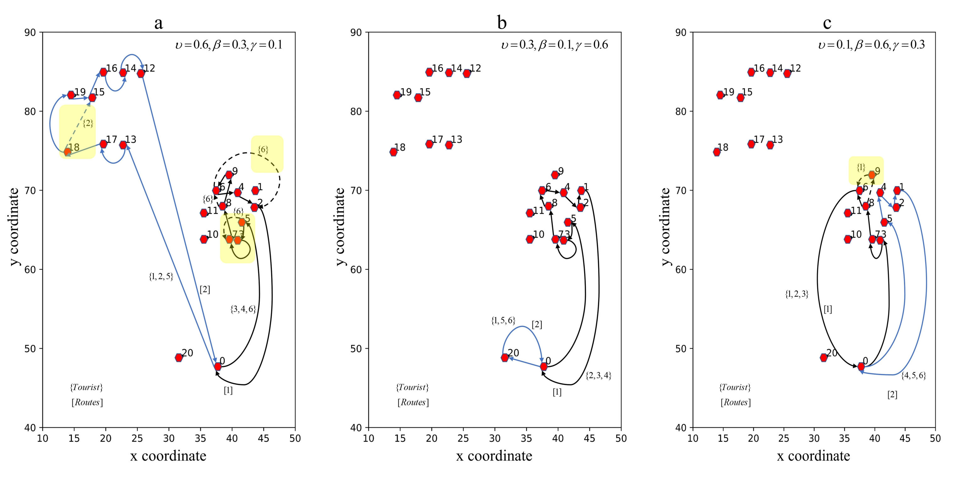
Solutions number 40, 76, and 124 are chosen to analyze the behaviour of the variations in the objectives and are represented in Table 4. In Figure 2, the routes generated with , , , and are shown.
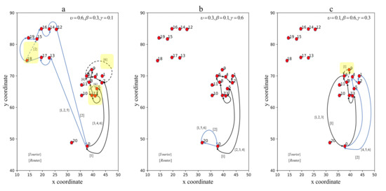
Figure 2.
Illustrative example of solutions. Comparison in the Cartesian plane of the routes obtained with weight variations ((a) = 0.6, = 0.3, = 0.1; (b) = 0.3, = 0.1, = 0.6; (c) = 0.1, = 0.6, = 0.3).
In Figure 2a, two routes are generated and three tourists are grouped in each . In tourists and visit additional POIs according to their preference. For example, after arrival at POI = 5 tourists and move to POI = 3 and then to POI = 7. However, tourist does not visit POI = 3, but goes from POI = 5 to POI = 7 directly. Different modes of transportation are used on this route. In arcs (3–7) and (5–3) tourists and use (bus). In the rest of the route, all tourists use (car). On the route the main mode of transport is . However, on arc (3–17) tourists , , and use , as does tourist on arc (17–18).
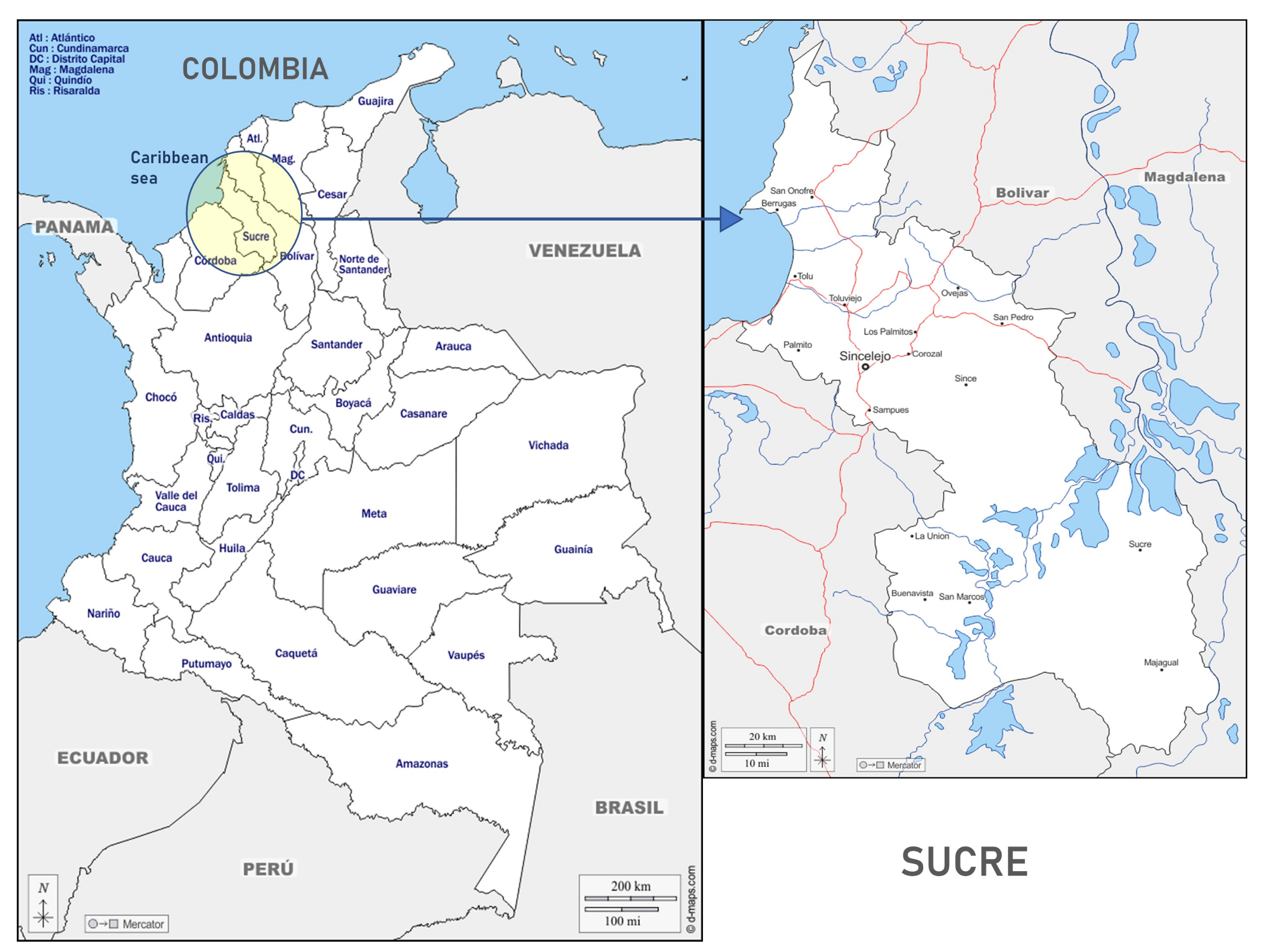
4.1. Case Study Area
This section applies the proposed model to a real case study to planning routes. In this case, we use the data of POIs of Sucre. The department of Sucre is located in the northern region of Colombia and borders the Caribbean Sea (see Figure 3). The territory is divided into five subregions (Golfo de Morrosquillo, Montes de María, La Mojana, Sabanas, and San Jorge), and each subregion attracts different categories of tourists. Different cultural, economic, social, and geographical aspects make Sucre a potentially rich tourist site. Tourist activities include sun and beach, nature, agrotourism, adventure, aqua tourism, religious, cultural, ecotourism, and gastronomy [103].
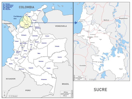
Figure 3.
Location of Sucre, Colombia.
The real instance Toptw-jMund-d was selected for the application of the model in our case study. This instance has 13 POIs including the starting node (0). We selected a small instance because the complexity of the model does not allow exact solutions with larger instances to be found in a reasonable amount of time, as shown in Table 4. This instance considers a total of four tourists with maximum travel time min. The budgets for each tourist are 10,000, 8000, 10,000, 10,000, respectively. The costs per km according to the mode of transport ( = car and bus) are and , respectively. This instance belongs to the set of 16 instances with the available tourist information of Sucre. The POIs belong to the tourist corridor of the Golfo de Morrosquillo and Sabanas subregions, which includes eight municipalities. In total, 201 POIs are catalogued (including the starting node 0) associated with sun and beach tourism , culture , religious , aquatourism , and adventure, nature, and ecotourism [104]. The instances correspond to each municipality (Toptw-jMun (a, b, c, d, e, f, g, h)), type of tourism (Toptw-jClass (a, b, c, d, e)), subregion (Toptw-jSubR (a, b)), and tourist corridor (Toptw-jGen).
Next, three scenarios are developed to observe the behaviour of the model. (i). Sustainability; (ii). Sustainability and uncertainty; (iii). Variation of preferences. The first scenario compares obtained solutions where the benefit of the tourists is prioritised, with another that aims to reduce the emissions of CO . The second scenario compares obtained solutions in with another itinerary under uncertainty . Finally, the last scenario generates a variation of the preference matrix of to obtain new itinerary .
4.1.1. Sustainability
In this scenario, we compare the routes resulting from the sets of weights and for , , and , respectively. The values of , , , and are set to 1.
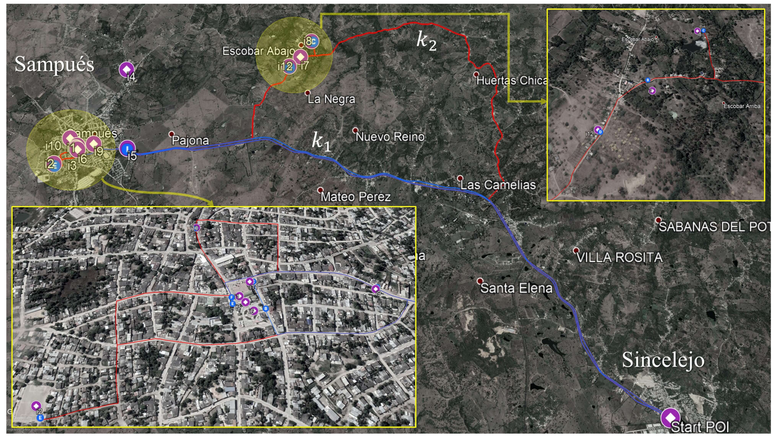
The behaviour of the routes shows a significant change when CO emissions are prioritised with respect to individual profit. The itinerary prioritises the inclusion of the highest number of POIs in the route to increase . However, emissions reach a total of and the difference between the profits of tourists corresponds to . The solution is shown in Figure 4. Route assigned to tourists and performs the sequence . Route assigned to tourists and evidence of extra POIs visited by some tourists. Tourist performs the sequence , while tourist performs . The use of the transport mode predominates. Transport mode is only used in arcs , , , and .
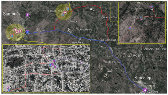
Figure 4.
First itinerary. This figure shows the itinerary for .
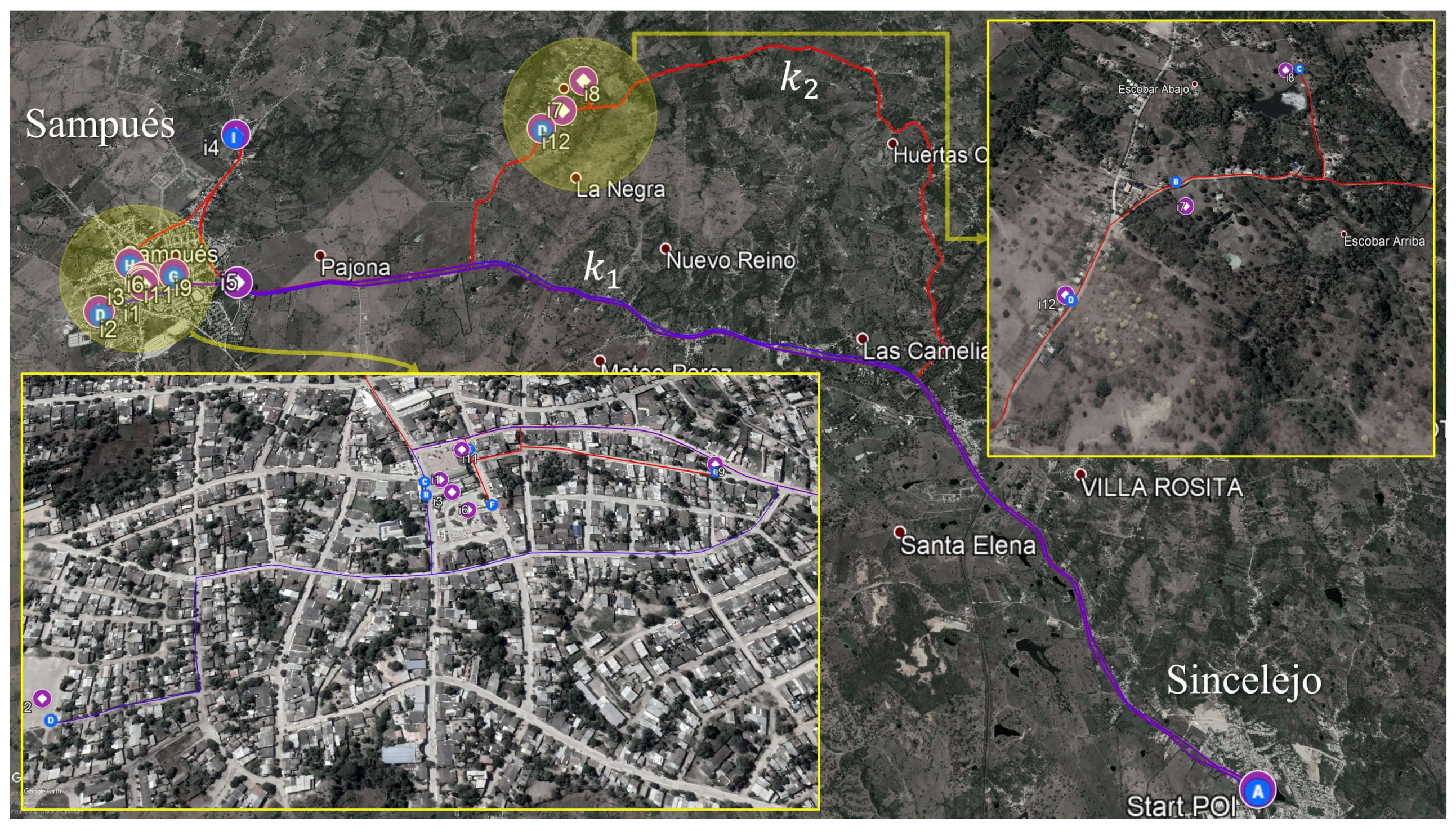
Compared to , the solutions in itinerary minimises the consumption and costs of CO emissions. The objective values are , , and . The cost of emissions decreases by while the individual profits only decrease by . Similarly, group equity improves, decreasing the difference in earnings by . The solution is shown in Figure 5. In this itinerary, all the POIs are also visited. The groups of tourists assigned to each route visit the same points. The mode of transport used is .
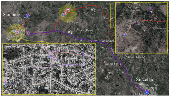
Figure 5.
Second itinerary. This figure shows the itinerary for .
4.1.2. Sustainability and Uncertainty
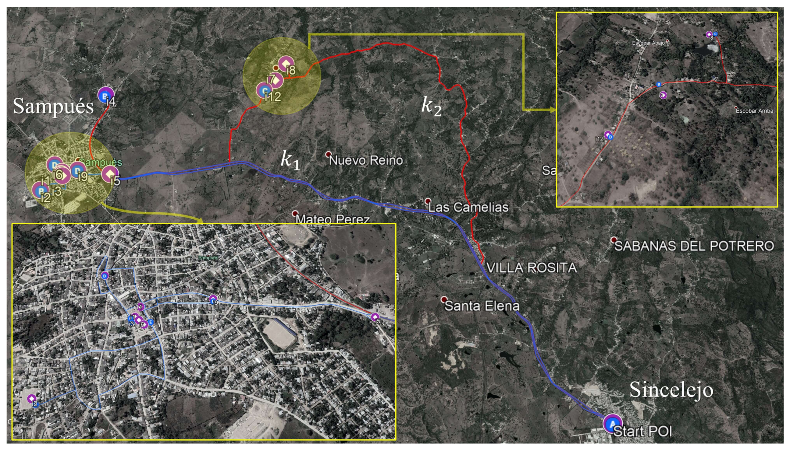
In this scenario, a variation of the values of the -cuts is performed to obtain the itinerary . The highest degree of variation is assigned and . The solution is shown in Figure 6. Compared to the itinerary a higher individual profit is achieved with . However, the equity of the group decreases and increases the emissions only by . Diversification of POIs visited is generated for tourists and where in route POIs and , were assigned, respectively. The mode of transport used throughout the route is .
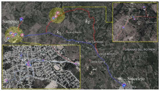
Figure 6.
variation. This figure shows the itinerary for .
4.1.3. Variation of Preferences
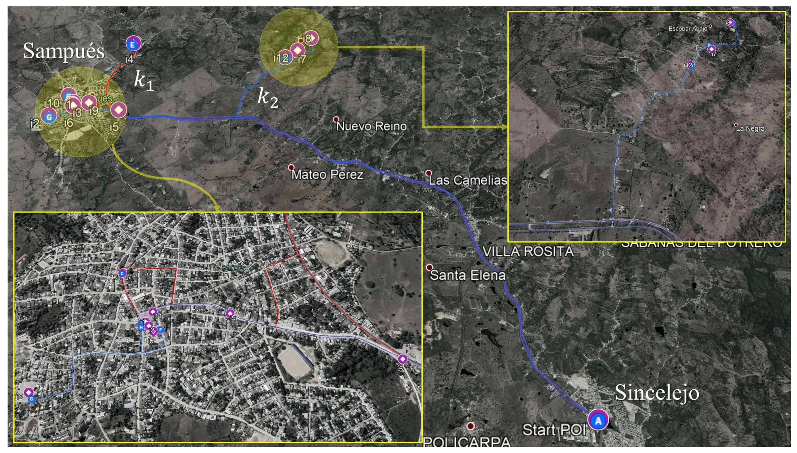
In this last scenario, the itinerary is compared with those obtained in a new . The initial matrix of preferences based on the triangular numbers is changed to the matrix, containing a new set of preference (triangular numbers). The route obtained is shown in Figure 7. Changing preferences directly affects the result. However, no tourist visits any extra POIs in the new itinerary. The goal values are , , and . The and preference arrays are shown in Table 5.

Figure 7.
Preferences shifts. This figure shows the itinerary for para .
Table 5.
Preferences. Variation in the preference limits in the comparison of the two scenarios.
5. Conclusions
Tourism management should be oriented towards the development of sustainability to influence the scope of the Sustainable Development Goals and strengthen economic reactivation. Transport plays a fundamental role in tourist destinations and route planning is directly linked to this activity. Transport also has a significant influence on CO emissions and negative environmental externalities. The developed model aims to minimise CO emissions generated by multi-modal transport used by tourists on their routes. Another critical aspect of sustainability is the social dimension. Our model takes into account this dimension from the equity of distribution. It generates routes that equally benefit all the tourists in the group. These contributions are novel in the TTDP literature and allow including social and environmental dimensions from an operational research approach. In this sense, the model’s objectives are summarised as follows: (i). maximise the individual benefit of tourists; (ii). maximise group equity by minimising the difference in individual benefits; (iii). minimise CO emissions. Our model provides the management of sustainable planning that can translate into advantages for the tourism supply chain; considering sustainability in the framework of tourism processes can significantly benefit organisations. The main effects reflect an increase in consumption, investment, number of arrivals, growth opportunities, among other benefits generated by stakeholders.
The proposed model also considers some components with uncertainty and approaches the problem from the perspective of fuzzy optimisation. In particular, this model considers the individual preferences of tourists, the budget and time available for the trip, and imprecise, vague, and flexible travel times. Auxiliary models were used to find feasible solutions with fuzzy time window constraints and travel times. The objective function (objectives Z and Z) with fuzzy costs is addressed using the Adamo index as the ordering function.
Additionally, under the conditions of the COVID-19 pandemic, the model presents an alternative for the construction of itineraries that organise routes respecting a maximum capacity. Therefore, it avoids the agglomeration of tourists at sites of interest. Likewise, the transport selection represents an important option since tourists can select a private means of transport to prevent contagion on public transport.
The set of tests demonstrate the complexity of the model. Instances of up to 21 nodes, two modes of transport, six tourists, and two routes were used for the experimentation. A total of 300 tests were performed with variations in target weights and -cuts. The variation of the weights of the objectives shows that increasing Z increases Z and Z. That is, as individual profit increases, emissions and the equity gap of the group increase. However, in the real-world applied case, the solution reflects a more environmentally friendly route without significantly reducing individual benefits and increasing the group equity gap. Finally, in the fuzzy components, with a certain degree of tolerance, the variation of the -cuts diversifies the results mainly for Z and Z, which is consistent with the fuzzy nature of the model.
Future research lines need to develop algorithms using meta-heuristic techniques to find solutions at reasonable execution times and thus apply our approach with medium and large size instances. In real-world cases, we can see situations with a more significant number of POIs to plan routes and the demand of users to have applications to obtain quick solutions. The methodology must have the capacity to generate solutions in low and efficient computational times. Furthermore, waiting times between visits at POIs to apply disinfection and bio-security schemes may be considered due to the current pandemic conditions. These times can also be considered uncertain. Finally, the information obtained by the model can be used as input data for simulation models to review prospective policies for economic recovery.
Author Contributions
Conceptualization, J.R.-M. and J.B.; methodology, J.R.-M., J.B. and J.R.M.-T.; experiments, J.R.-M.; validation, J.R.-M., J.B. and J.R.M.-T.; formal analysis, J.R.-M., J.B. and J.R.M.-T.; investigation, J.R.-M.; data curation, J.R.-M.; writing—original draft preparation, J.R.-M. and J.B.; writing—review and editing, J.R.-M., J.B. and J.R.M.-T.; supervision, J.R.M.-T. and J.B. All authors have read and agreed to the published version of the manuscript.
Funding
The work presented in this paper is partially funded under Doctoral Scholarship “Carlos Jordana” from the School of Engineering at Universidad de La Sabana (project INGPhD-37-2020), by a scholarship from the Colombian Ministry of Science, Technology, and Innovation, and by the Spanish Ministry of Science and Innovation (PID2019-104410RB-I00).
Institutional Review Board Statement
Not applicable.
Informed Consent Statement
Not applicable.
Data Availability Statement
Data employed to run the experiments are available from the corresponding author upon request.
Conflicts of Interest
The authors declare no conflict of interest. The funders had no role in the design of the study; in the collection, analyses, or interpretation of data; in the writing of the manuscript, or in the decision to publish the results.
References
- Delgado, M.; Mills, K.G. The supply chain economy: A new industry categorization for understanding innovation in services. Res. Policy 2020, 49, 104039. [Google Scholar] [CrossRef]
- The World Bank. World Development Indicators: Structure of Output; Technical Report; The World Bank: Washington, DC, USA, 2021. [Google Scholar]
- Lee, H.K.; Fernando, Y. The antecedents and outcomes of the medical tourism supply chain. Tour. Manag. 2015, 46, 148–157. [Google Scholar] [CrossRef]
- Daniel, A.D.; Costa, R.A.; Pita, M.; Costa, C. Tourism Education: What about entrepreneurial skills? J. Hosp. Tour. Manag. 2017, 30, 65–72. [Google Scholar] [CrossRef]
- Kanda, W.; Kivimaa, P. What opportunities could the COVID-19 outbreak offer for sustainability transitions research on electricity and mobility? Energy Res. Soc. Sci. 2020, 68, 101666. [Google Scholar] [CrossRef]
- Lokhandwala, S.; Gautam, P. Indirect impact of COVID-19 on environment: A brief study in Indian context. Environ. Res. 2020, 188, 109807. [Google Scholar] [CrossRef] [PubMed]
- Shakil, M.H.; Munim, Z.H.; Tasnia, M.; Sarowar, S. COVID-19 and the environment: A critical review and research agenda. Sci. Total Environ. 2020, 745, 141022. [Google Scholar] [CrossRef]
- Bertella, G. Re-thinking sustainability and food in tourism. Ann. Tour. Res. 2020, 84, 103005. [Google Scholar] [CrossRef] [PubMed]
- Higgins-Desbiolles, F. Socialising tourism for social and ecological justice after COVID-19. Tour. Geogr. 2020, 22, 610–623. [Google Scholar] [CrossRef] [Green Version]
- Hall, C.M. Constructing sustainable tourism development: The 2030 agenda and the managerial ecology of sustainable tourism. J. Sustain. Tour. 2019, 27, 1044–1060. [Google Scholar] [CrossRef]
- Nguyen, T.Q.T.; Young, T.; Johnson, P.; Wearing, S. Conceptualising networks in sustainable tourism development. Tour. Manag. Perspect. 2019, 32, 100575. [Google Scholar] [CrossRef]
- Gong, M.; Gao, Y.; Koh, L.; Sutcliffe, C.; Cullen, J. The role of customer awareness in promoting firm sustainability and sustainable supply chain management. Int. J. Prod. Econ. 2019, 217, 88–96. [Google Scholar] [CrossRef]
- Park, B.I.; Ghauri, P.N. Determinants influencing CSR practices in small and medium sized MNE subsidiaries: A stakeholder perspective. J. World Bus. 2015, 50, 192–204. [Google Scholar] [CrossRef]
- Scott, D.; Hall, C.M.; Gössling, S. Global tourism vulnerability to climate change. Ann. Tour. Res. 2019, 77, 49–61. [Google Scholar] [CrossRef]
- Wolf, F.; Filho, W.L.; Singh, P.; Scherle, N.; Reiser, D.; Telesford, J.; Miljković, I.B.; Havea, P.H.; Li, C.; Surroop, D.; et al. Influences of Climate Change on Tourism Development in Small Pacific Island States. Sustainability 2021, 13, 4223. [Google Scholar] [CrossRef]
- Scott, D.; Gössling, S.; Hall, C.M. International tourism and climate change. WIREs Clim. Chang. 2012, 3, 213–232. [Google Scholar] [CrossRef]
- Loehr, J.; Becken, S. The Tourism Climate Change Knowledge System. Ann. Tour. Res. 2021, 86, 103073. [Google Scholar] [CrossRef]
- Qian, J.; Eglese, R. Fuel emissions optimization in vehicle routing problems with time-varying speeds. Eur. J. Oper. Res. 2016, 248, 840–848. [Google Scholar] [CrossRef]
- Peeters, P.; Dubois, G. Tourism travel under climate change mitigation constraints. J. Transp. Geogr. 2010, 18, 447–457. [Google Scholar] [CrossRef]
- Le-Klähn, D.T.; Hall, C.M. Tourist use of public transport at destinations—A review. Curr. Issues Tour. 2014, 18, 785–803. [Google Scholar] [CrossRef]
- Sedarati, P.; Santos, S.; Pintassilgo, P. System Dynamics in Tourism Planning and Development. Tour. Plan. Dev. 2018, 16, 256–280. [Google Scholar] [CrossRef]
- Kotiloglu, S.; Lappas, T.; Pelechrinis, K.; Repoussis, P. Personalized multi-period tour recommendations. Tour. Manag. 2017, 62, 76–88. [Google Scholar] [CrossRef] [Green Version]
- Vansteenwegen, P.; Oudheusden, D.V. The Mobile Tourist Guide: An OR Opportunity. OR Insight 2007, 20, 21–27. [Google Scholar] [CrossRef]
- Brito, J.; Expósito, A.; Moreno, J.A. A fuzzy GRASP algorithm for solving a Tourist Trip Design Problem. In Proceedings of the 2017 IEEE International Conference on Fuzzy Systems (FUZZ-IEEE), Naples, Italy, 9–12 July 2017. [Google Scholar] [CrossRef]
- Expósito, A.; Mancini, S.; Brito, J.; Moreno, J.A. A fuzzy GRASP for the tourist trip design with clustered POIs. Expert Syst. Appl. 2019, 127, 210–227. [Google Scholar] [CrossRef]
- Garcia, A.; Arbelaitz, O.; Linaza, M.T.; Vansteenwegen, P.; Souffriau, W. Personalized Tourist Route Generation. In Current Trends in Web Engineering; Springer: Berlin/Heidelberg, Germany, 2010; pp. 486–497. [Google Scholar] [CrossRef] [Green Version]
- Ruiz-Meza, J.; Montoya-Torres, J.R. A systematic literature review for the tourist trip design problem: Extensions, solution techniques and future research lines. Compt. Oper. Res. 2021. submitted for publication. [Google Scholar]
- Souffiau, W.; Maervoet, J.; Vansteenwegen, P.; Berghe, G.V.; Oudheusden, D.V. A Mobile Tourist Decision Support System for Small Footprint Devices. In Lecture Notes in Computer Science; Springer: Berlin/Heidelberg, Germany, 2009; pp. 1248–1255. [Google Scholar] [CrossRef]
- Zheng, W.; Liao, Z. Using a heuristic approach to design personalized tour routes for heterogeneous tourist groups. Tour. Manag. 2019, 72, 313–325. [Google Scholar] [CrossRef]
- Wang, W.; Liu, J.; Innes, J.L. Conservation equity for local communities in the process of tourism development in protected areas: A study of Jiuzhaigou Biosphere Reserve, China. World Dev. 2019, 124, 104637. [Google Scholar] [CrossRef]
- Arowoshegbe, A.O.; Uniamikogbo, E. Sustainability and Triple Bottom Line: An Overview of Two Interrelated Concepts. Igbinedion Univ. J. Account. 2016, 2, 88–126. [Google Scholar]
- D’Eusanio, M.; Serreli, M.; Zamagni, A.; Petti, L. Assessment of social dimension of a jar of honey: A methodological outline. J. Clean. Prod. 2018, 199, 503–517. [Google Scholar] [CrossRef]
- Kloepffer, W. Life cycle sustainability assessment of products. Int. J. Life Cycle Assess. 2008, 13, 89–95. [Google Scholar] [CrossRef]
- Vega-Mejía, C.A.; Montoya-Torres, J.R.; Islam, S.M.N. Consideration of triple bottom line objectives for sustainability in the optimization of vehicle routing and loading operations: A systematic literature review. Ann. Oper. Res. 2017, 273, 311–375. [Google Scholar] [CrossRef]
- Yeh, D.Y.; Cheng, C.H. Recommendation system for popular tourist attractions in Taiwan using Delphi panel and repertory grid techniques. Tour. Manag. 2015, 46, 164–176. [Google Scholar] [CrossRef]
- Zhang, X.; Song, H.; Huang, G.Q. Tourism supply chain management: A new research agenda. Tour. Manag. 2009, 30, 345–358. [Google Scholar] [CrossRef] [Green Version]
- Karunakaran, D.; Mei, Y.; Zhang, M. Multitasking Genetic Programming for Stochastic Team Orienteering Problem with Time Windows. In Proceedings of the 2019 IEEE Symposium Series on Computational Intelligence (SSCI), Xiamen, China, 6–9 December 2019. [Google Scholar] [CrossRef]
- Zheng, W.; Liao, Z.; Lin, Z. Navigating through the complex transport system: A heuristic approach for city tourism recommendation. Tour. Manag. 2020, 81, 104162. [Google Scholar] [CrossRef]
- Jaber, H.; Marle, F.; Vidal, L.A.; Sarigol, I.; Didiez, L. A Framework to Evaluate Project Complexity Using the Fuzzy TOPSIS Method. Sustainability 2021, 13, 3020. [Google Scholar] [CrossRef]
- Javanmardi, E.; Liu, S.; Xie, N. Exploring Grey Systems Theory-Based Methods and Applications in Sustainability Studies: A Systematic Review Approach. Sustainability 2020, 12, 4437. [Google Scholar] [CrossRef]
- Jiang, P.; Yang, H.; Li, R.; Li, C. Inbound tourism demand forecasting framework based on fuzzy time series and advanced optimization algorithm. Appl. Soft Comput. 2020, 92, 106320. [Google Scholar] [CrossRef]
- Lok, W.J.; Ng, L.Y.; Andiappan, V. Optimal decision-making for combined heat and power operations: A fuzzy optimisation approach considering system flexibility, environmental emissions, start-up and shutdown costs. Process Saf. Environ. Prot. 2020, 137, 312–327. [Google Scholar] [CrossRef]
- Zhang, S.; Chen, M.; Zhang, W.; Zhuang, X. Fuzzy optimization model for electric vehicle routing problem with time windows and recharging stations. Expert Syst. Appl. 2020, 145, 113123. [Google Scholar] [CrossRef]
- Susanty, A.; Puspitasari, N.B.; Saptadi, S.; Prasetyo, S. Implementation of green tourism concept through a dynamic programming algorithm to select the best route of tourist travel. IOP Conf. Ser. Earth Environ. Sci. 2018, 195, 012035. [Google Scholar] [CrossRef]
- Gunawan, A.; Lau, H.C.; Vansteenwegen, P. Orienteering Problem: A survey of recent variants, solution approaches and applications. Eur. J. Oper. Res. 2016, 255, 315–332. [Google Scholar] [CrossRef]
- Kaushal, V.; Sharma, S.; Reddy, G.M. A structural analysis of destination brand equity in mountainous tourism destination in northern India. Tour. Hosp. Res. 2018, 19, 452–464. [Google Scholar] [CrossRef]
- Ravald, A.; Grönroos, C. The value concept and relationship marketing. Eur. J. Mark. 1996, 30, 19–30. [Google Scholar] [CrossRef]
- Michael, N.; Reisinger, Y.; Hayes, J.P. The UAE’s tourism competitiveness: A business perspective. Tour. Manag. Perspect. 2019, 30, 53–64. [Google Scholar] [CrossRef]
- Arbolino, R.; Yigitcanlar, T.; L’Abbate, P.; Ioppolo, G. Effective growth policymaking: Estimating provincial territorial development potentials. Land Use Policy 2019, 86, 313–321. [Google Scholar] [CrossRef]
- Truong, N.V.; Shimizu, T. The effect of transportation on tourism promotion: Literature review on application of the Computable General Equilibrium (CGE) Model. Transp. Res. Procedia 2017, 25, 3096–3115. [Google Scholar] [CrossRef]
- Belgin, O.; Karaoglan, I.; Altiparmak, F. Two-echelon vehicle routing problem with simultaneous pickup and delivery: Mathematical model and heuristic approach. Comput. Ind. Eng. 2018, 115, 1–16. [Google Scholar] [CrossRef]
- Bektaş, T.; Laporte, G. The Pollution-Routing Problem. Transp. Res. Part B Methodol. 2011, 45, 1232–1250. [Google Scholar] [CrossRef]
- Palmer, A. The Developement of an Integrated Routing and Carbon Dioxide Emissions Model for Goods Vehicle. Ph.D. Thesis, Cranfield University, Cranfield, UK, November 2007. [Google Scholar]
- Kara, İ.; Kara, B.Y.; Yetis, M.K. Energy Minimizing Vehicle Routing Problem. In Combinatorial Optimization and Applications; Springer: Berlin/Heidelberg, Germany, 2007; pp. 62–71. [Google Scholar] [CrossRef]
- Gavalas, D.; Konstantopoulos, C.; Mastakas, K.; Pantziou, G.; Vathis, N. Heuristics for the time dependent team orienteering problem: Application to tourist route planning. Comput. Oper. Res. 2015, 62, 36–50. [Google Scholar] [CrossRef]
- Gangoiti, A.G.; Arbelaitz, O.; Otaegui, O.; Vansteenwegen, P.; Linaza, M.T. Public Transportation Algorithm for an Intelligent Routing System. In Proceedings of the 16th ITS World Congress and Exhibition on Intelligent Transport Systems and Services, Stockholm, Sweden, 21–25 September 2009. [Google Scholar]
- Churchill, S.A.; Inekwe, J.; Ivanovski, K.; Smyth, R. Transport infrastructure and CO2 emissions in the OECD over the long run. Transp. Res. Part D Transp. Environ. 2021, 95, 102857. [Google Scholar] [CrossRef]
- Abbaspour, R.; Samadzadeg, F. Itinerary Planning in Multimodal Urban Transportation Network. J. Appl. Sci. 2009, 9, 1898–1906. [Google Scholar] [CrossRef]
- Garcia, A.; Arbelaitz, O.; Vansteenwegen, P.; Souffriau, W.; Linaza, M.T. Hybrid Approach for the Public Transportation Time Dependent Orienteering Problem with Time Windows. In Lecture Notes in Computer Science; Springer: Berlin/Heidelberg, Germany, 2010; pp. 151–158. [Google Scholar] [CrossRef]
- Abbaspour, R.A.; Samadzadegan, F. Time-dependent personal tour planning and scheduling in metropolises. Expert Syst. Appl. 2011, 38, 12439–12452. [Google Scholar] [CrossRef]
- Garcia, A.; Vansteenwegen, P.; Arbelaitz, O.; Souffriau, W.; Linaza, M.T. Integrating public transportation in personalised electronic tourist guides. Comput. Oper. Res. 2013, 40, 758–774. [Google Scholar] [CrossRef]
- Gavalas, D.; Kasapakis, V.; Konstantopoulos, C.; Pantziou, G.; Vathis, N.; Zaroliagis, C. The eCOMPASS multimodal tourist tour planner. Expert Syst. Appl. 2015, 42, 7303–7316. [Google Scholar] [CrossRef]
- Wu, X.; Guan, H.; Han, Y.; Ma, J. A tour route planning model for tourism experience utility maximization. Adv. Mech. Eng. 2017, 9, 168781401773230. [Google Scholar] [CrossRef] [Green Version]
- Yu, V.F.; Jewpanya, P.; Ting, C.J.; Redi, A.P. Two-level particle swarm optimization for the multi-modal team orienteering problem with time windows. Appl. Soft Comput. 2017, 61, 1022–1040. [Google Scholar] [CrossRef]
- Liao, Z.; Zheng, W. Using a heuristic algorithm to design a personalized day tour route in a time-dependent stochastic environment. Tour. Manag. 2018, 68, 284–300. [Google Scholar] [CrossRef]
- Zhang, R.; Liu, Z.; Feng, X. A novel flexible shuttle vehicle scheduling problem in scenic areas: Task-divided graph-based formulation and ALGORITHM. Comput. Ind. Eng. 2021, 156, 107295. [Google Scholar] [CrossRef]
- Kargar, M.; Lin, Z. A socially motivating and environmentally friendly tour recommendation framework for tourist groups. Expert Syst. Appl. 2021, 180, 115083. [Google Scholar] [CrossRef]
- Ntakolia, C.; Iakovidis, D.K. A swarm intelligence graph-based pathfinding algorithm (SIGPA) for multi-objective route planning. Comput. Oper. Res. 2021, 133, 105358. [Google Scholar] [CrossRef]
- Wang, Y.W.; Lin, C.C.; Lee, T.J. Electric vehicle tour planning. Transp. Res. Part D Transp. Environ. 2018, 63, 121–136. [Google Scholar] [CrossRef]
- Karbowska-Chilinska, J.; Chociej, K. Optimization of Multistage Tourist Route for Electric Vehicle. In Advances in Intelligent Systems and Computing; Springer International Publishing: Cham, Switzerland, 2019; pp. 186–196. [Google Scholar] [CrossRef]
- Karbowska-Chilinska, J.; Chociej, K. Genetic Algorithm for Generation Multistage Tourist Route of Electrical Vehicle. In Computer Information Systems and Industrial Management; Saeed, K., Dvorský, J., Eds.; Springer International Publishing: Cham, Switzerland, 2020; pp. 366–376. [Google Scholar]
- Sylejmani, K.; Dorn, J.; Musliu, N. Planning the trip itinerary for tourist groups. Inf. Technol. Tour. 2017, 17, 275–314. [Google Scholar] [CrossRef]
- Malucelli, F.; Giovannini, A.; Nonato, M. Designing Single Origin-destination Itineraries for Several Classes of Cycle-tourists. Transp. Res. Procedia 2015, 10, 413–422. [Google Scholar] [CrossRef] [Green Version]
- Friedman, R.S.; Law, E.A.; Bennett, N.J.; Ives, C.D.; Thorn, J.P.R.; Wilson, K.A. How just and just how? A systematic review of social equity in conservation research. Environ. Res. Lett. 2018, 13, 053001. [Google Scholar] [CrossRef]
- İlhan, T.; Iravani, S.M.R.; Daskin, M.S. The orienteering problem with stochastic profits. IIE Trans. 2008, 40, 406–421. [Google Scholar] [CrossRef]
- Amghar, M.; Zoullouti, B.; Sbiti, N. Risk Analysis of Operating Room Using the Fuzzy Bayesian Network Model. Int. J. Eng. 2017, 30, 66–74. [Google Scholar]
- Zheng, W.; Huang, X.; Li, Y. Understanding the tourist mobility using GPS: Where is the next place? Tour. Manag. 2017, 59, 267–280. [Google Scholar] [CrossRef] [Green Version]
- Jackson, J.; Mei, Y. Genetic Programming Hyper-heuristic with Cluster Awareness for Stochastic Team Orienteering Problem with Time Windows. In Proceedings of the 2020 IEEE Congress on Evolutionary Computation (CEC), Glasgow, UK, 19–24 July 2020. [Google Scholar] [CrossRef]
- Matsuda, Y.; Nakamura, M.; Kang, D.; Miyagi, H. An optimal routing problem for sightseeing with fuzzy tilme-varying weights. In Proceedings of the 2004 IEEE International Conference on Systems, Man and Cybernetics (IEEE Cat. No.04CH37583), The Hague, The Netherlands, 10–13 October 2004. [Google Scholar] [CrossRef]
- Hasuike, T.; Katagiri, H.; Tsubaki, H. Tour route planning problem for sightseeing with the multiroute under several uncertain conditions. In Proceedings of the 2012 IEEE International Conference on Systems, Man, and Cybernetics (SMC), Seoul, Korea, 14–17 October 2012. [Google Scholar] [CrossRef]
- Hasuike, T.; Katagiri, H.; Tsubaki, H.; Tsuda, H. Route planning problem under fuzzy sightseeing times and satisfaction values of sightseeing places. In Proceedings of the 2013 Joint IFSA World Congress and NAFIPS Annual Meeting (IFSA/NAFIPS), Edmonton, AB, Canada, 24–28 June 2013. [Google Scholar] [CrossRef]
- Hasuike, T.; Katagiri, H.; Tsubaki, H.; Tsuda, H. Flexible route planning for sightseeing with fuzzy random and fatigue-dependent satisfactions. J. Adv. Comput. Intell. Intell. Inform. 2014, 18, 190–196. [Google Scholar] [CrossRef]
- Expósito, A.; Mancini, S.; Brito, J.; Moreno, J.A. Uncertainty Management with Fuzzy and Rough Sets. In Chapter Solving a Fuzzy Tourist Trip Design Problem with Clustered Points of Interest; Springer International Publishing: Cham, Switzerland, 2019. [Google Scholar] [CrossRef]
- Ariyarit, A.; Kanazaki, M.; Bureerat, S. An Approach Combining an Efficient and Global Evolutionary Algorithm with a Gradient-Based Method for Airfoil Design Problems. Smart Sci. 2020, 8, 14–23. [Google Scholar] [CrossRef]
- Trachanatzi, D.; Rigakis, M.; Marinaki, M.; Marinakis, Y. An interactive preference-guided firefly algorithm for personalized tourist itineraries. Expert Syst. Appl. 2020, 159, 113563. [Google Scholar] [CrossRef]
- Arbolino, R.; Boffardi, R.; Simone, L.D.; Ioppolo, G. Multi-objective optimization technique: A novel approach in tourism sustainability planning. J. Environ. Manag. 2021, 285, 112016. [Google Scholar] [CrossRef]
- Yan, L.; Gao, B.W.; Zhang, M. A mathematical model for tourism potential assessment. Tour. Manag. 2017, 63, 355–365. [Google Scholar] [CrossRef]
- Ishizaka, A.; Nemery, P.; Lidouh, K. Location selection for the construction of a casino in the Greater London region: A triple multi-criteria approach. Tour. Manag. 2013, 34, 211–220. [Google Scholar] [CrossRef] [Green Version]
- Bellman, R.E.; Zadeh, L.A. Decision-Making in a Fuzzy Environment. Manag. Sci. 1970, 17, B-141–B-164. [Google Scholar] [CrossRef]
- Verdegay, J.L. Fuzzy optimization: Models, methods and perspectives. In Proceedings of the 6th IFSA-95 World Congress, Sao Paulo, Brazil, 22–28 July 1995; pp. 39–71. [Google Scholar]
- Delgado, M.; Verdegay, J.; Vila, M. A general model for fuzzy linear programming. Fuzzy Sets Syst. 1989, 29, 21–29. [Google Scholar] [CrossRef]
- Ruiz-Meza, J.; Montoya-Torres, J.R. Tourist trip design with heterogeneous preferences, transport mode selection and environmental considerations. Ann. Oper. Res. 2021. [Google Scholar] [CrossRef] [PubMed]
- Jafari, R.; Yu, W.; Razvarz, S.; Gegov, A. Numerical methods for solving fuzzy equations: A survey. Fuzzy Sets Syst. 2021, 404, 1–22. [Google Scholar] [CrossRef]
- Kaufmann, A.; Gupta, M.M. Fuzzy Mathematical Models in Engineering and Management Science; Elsevier Science Inc.: Amsterdam, The Netherlands, 1988. [Google Scholar]
- Adamo, J. Fuzzy decision trees. Fuzzy Sets Syst. 1980, 4, 207–219. [Google Scholar] [CrossRef]
- Herrera, F.; Verdegay, J. Fuzzy boolean programming problems with fuzzy costs: A general study. Fuzzy Sets Syst. 1996, 81, 57–76. [Google Scholar] [CrossRef]
- Hill, N.; Karagianni, E.; Jones, L.; MacCarthy, J.; Bonifazi, E.; Hinton, S.; Walker, C.; Harris, B. 2019 Government Greenhouse Gas Conversion Factors for Company Reporting. Methodologhy Paper for Emission Factors; Deparment for Business, Energy and Industrial Strategy: Kew, London, UK, 2019; Available online: https://www.gov.uk/government/publications/greenhouse-gas-reporting-conversion-factors-2019 (accessed on 16 February 2021)Technical Report.
- Fontaras, G.; Zacharof, N.G.; Ciuffo, B. Fuel consumption and CO2 emissions from passenger cars in Europe—Laboratory versus real-world emissions. Prog. Energy Combust. Sci. 2017, 60, 97–131. [Google Scholar] [CrossRef]
- Zacharof, N.; Fontaras, G.; Ciuffo, B.; Tsiakmakis, S.; Anagnostopoulos, K.; Marotta, A.; Pavlovic, J. Review of in Use Factors Affecting the Fuel Consumption and CO2 Emissions of Passenger Cars.; European Commission Joint Research Centre: Luxembourg, 2016. [Google Scholar] [CrossRef]
- SENDECO2. Precios de CO2. 2020. Available online: https://www.sendeco2.com/es/precios-co2 (accessed on 8 February 2021).
- Diakoulaki, D.; Mavrotas, G.; Papayannakis, L. Determining objective weights in multiple criteria problems: The critic method. Comput. Oper. Res. 1995, 22, 763–770. [Google Scholar] [CrossRef]
- Zeleny, M. The Attribute-Dynamic Attitude Model (Adam). Manag. Sci. 1976, 23, 12–26. [Google Scholar] [CrossRef]
- Gobernación de Sucre. Fondo de Promoción Turística-Colombia. Plan Estratégico de Desarrollo Turístico de Sucre 2011–2020. Technical Report, Gobernación de Sucre. 2011. Available online: https://www.citur.gov.co/upload/publications/documentos/184.Plan~_Estrategico_de_Turismo_de_Sucre.pdf (accessed on 3 February 2021).
- Viceministerio de Turismo. Listado de Atractivos Turísticos de Sucre. 2020. Available online: http://www.sucre.gov.co~/turismo/ruta-competitiva-turismo-vacacional (accessed on 15 February 2020).

Publisher’s Note: MDPI stays neutral with regard to jurisdictional claims in published maps and institutional affiliations. |
© 2021 by the authors. Licensee MDPI, Basel, Switzerland. This article is an open access article distributed under the terms and conditions of the Creative Commons Attribution (CC BY) license (https://creativecommons.org/licenses/by/4.0/).