3.1. Crash Frequency Model
Table 1 provides a summary of the crash frequency models concerning road segment data. These were divided according to the physical characteristics of roads. The study found that the mean value of crash occurrence is 6.39 times, the segment length is 3.08 km, the lane width is 3.47 m, and the road with median is 33%. In terms of traffic volume, findings show that an average of 14,465 vehicles per day are on the streets, of which 16.33% are trucks. The maximum annual average daily traffic (AADT) is 339,248 vehicles per day. This value refers to the district of Thanya Buri and Klongluang of Prathum Tani province. This route is road no. 1 (Phahonyothin Road), which has 10–14 lanes with a barrier in the middle. This area is an economic and complex area. This means that there are many trip production and trip attractions including industry zones, complex residences, universities, and shopping malls. In addition, the road connects the biggest regions of Thailand including the “North” and the “Northeast.” The official report of the AADT on this road could be assessed by the Thailand Department of Highways [
46].
In
Table 2, the overdispersion parameter is significant (0.143, SD = 0.002,
t-statistic > 1.96). Therefore, it can be concluded that the NB fits that Poisson model. The result of Vuong statistic is 18.916 (
t-statistic > 1.96). It could be stated that the ZINB is proved to be more appropriate. In summary, the study found that the Akaike information criterion (AIC) values continuously decrease until the SZINB reaches the smallest value. Here, a small AIC value indicated a model with better fit [
12,
47]. However, this study was analyzed based on the spatial analysis model, which used correlation spatial data. Vaida and Blanchard [
48] suggested that the conditional Akaike information criterion (cAIC) was a more appropriate model than the ordinary AIC. The penalty term in cAIC is related to the effective degrees of freedom
[
49]. The cAIC allows for the comparison of models with different random effect structures. It likewise allows for the comparison of mixed-effect models with cluster-specific models where the parameters are fixed. The result of the cAIC shows that the SZINB is the smallest. This finding can be interpreted in such a way that the SZINB is the most-fitted model [
50].
The pseudo-R
2 of SZINB is relatively low because there are many variables (e.g., human factors, weather, lighting, traffic signs, and land use factors) that are not measured [
51]. However, the pseudo-R
2 of SZINB was still within the acceptable criteria of Mohammadi et al. [
52], Abdul Manan et al. [
53]. These authors all accepted the goodness of fit at 0.06.
The model results of SZINB (
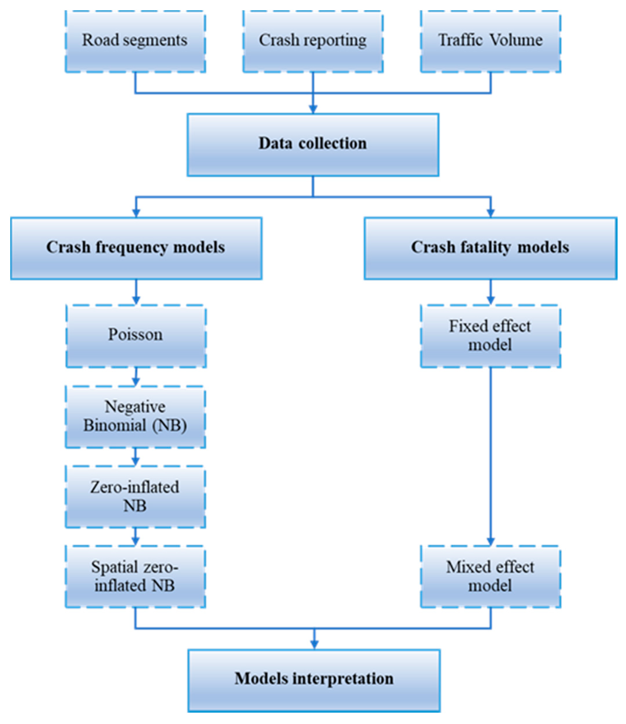
Table 3) were presented in three parts:
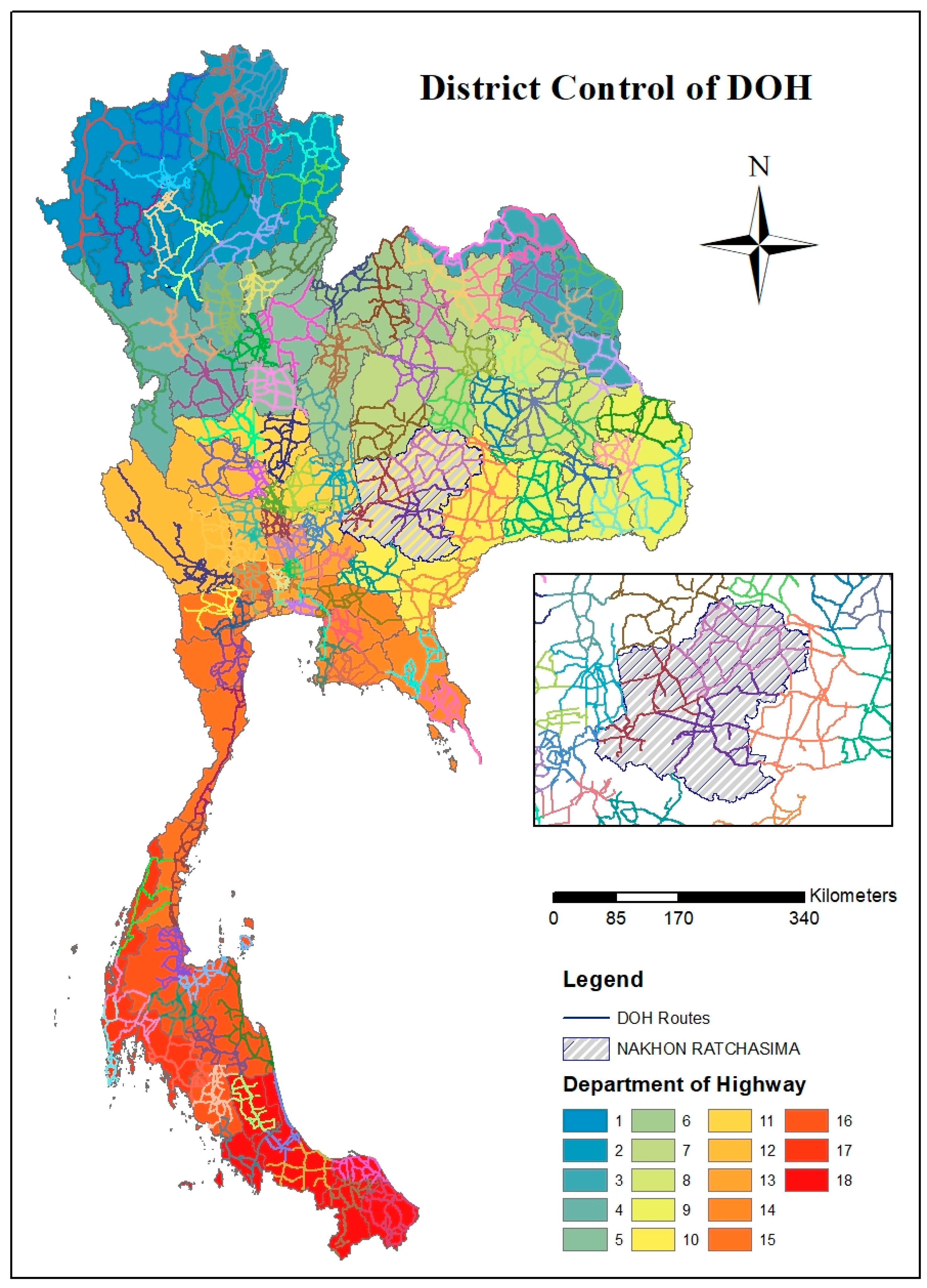
The random effect conditional model refers to the prediction of the relationship between the independent and dependent variables. These variables were grouped according to the sub-areas of the Department of Highway (DOH).
The normal state denotes the factors influencing collision number as non-zero state.
Lastly, zero state pertains to the factors that do not lead to crashes. The zero sate is modeled to find the significant variables that could be specifically led to be the zero-crash segment. These significant variables can be developed to be effective road safety policy.
The inverted signs between states mean that the factors positively or negatively affected the crash frequency. These factors include road length and LN_AADT. It is positive in a normal state and negative in a zero state. Thus, these variables were clearly interpreted to have increased crash frequency. This was expounded in the study of Dong et al. [
54].
According to the intercept of random effect, it is statistically significant and different from zero [
55]. This could mean that the crash frequencies vary across office highway districts. The variances of random effects for variables of road segment levels were found to be insignificant. In other words, the parameter estimation values were lower than those of the standard errors. Thus, the results indicate that such variables do not differently affect crash frequency in the sub-areas of the DOH. This finding is consistent with the study done by Aguero-Valverde [
28]. He found that the random effects of spatial error were not significant. The fact that the variance of random effect was not significant could be explained by the highway district office having no different control power on distance. As such, the traffic volume and the proportion of trucks were not significantly different in each area under each highway district office’s responsibility. Therefore, a management policy that aims to reduce the number of crashes can be uniformly applied throughout the country.
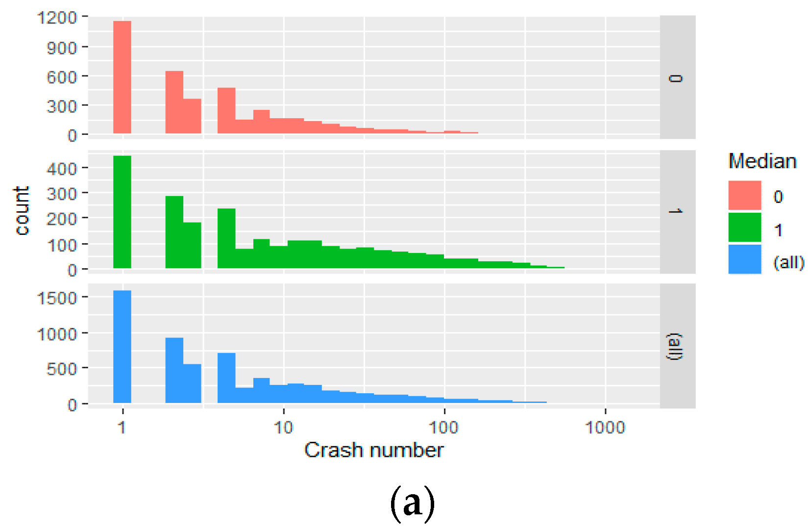
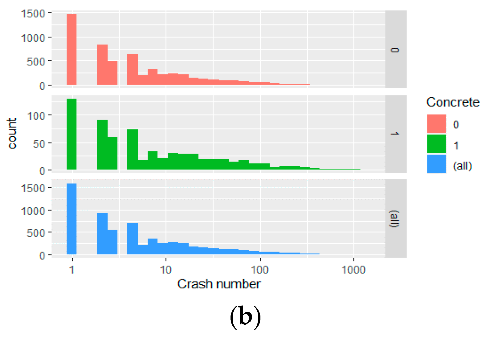
Traffic volume and the presence of road medians were the top factors that lead to crash occurrences. The reason behind this notion is that these two variables are clearly related. Roads with high volumes of traffic and that are built with medians subsequently lead to increased chances of crashes. Aguero-Valverde [
56], Liu et al. [
57] provided relevant study results. The reason why the existence of traffic islands caused more crashes could be explained by the fact that the Department of Thai Highways designed roads according to their traffic volume [
58]. Roads with traffic islands are usually roads with high traffic volume [
57]. Road shoulder and the traffic island width are other factors that contribute to car crashes. These results were inconsistent with those of Joon-Ki et al. [
8], which suggested that roads with narrow shoulders led to more frequency of trailing. However, for developing countries, Mahmud et al. [
31] found that shoulders did not contribute to more frequent crashes. As for the relationship of these two factors with traffic volume, it was found that the two factors positively correlated with traffic volume (
Figure 4). Nevertheless, these two factors should be further investigated to discover why increasing road width of traffic islands and shoulders increased the crash frequency in Thailand.
For zero states, the majority of negative values indicated that significant factors typically lead to an increase in crash frequency. For example, the increasing distance between road segments can lead to the non-zero state, followed by the existence of medians and increase in traffic volume [
56]. In view of the intercept of zero states, it was clearly found that it had a significant positive effect on a non-crashes. This implied that the mean frequency of crashes on each road segment was zero. Meanwhile, most of these factors led to a negative effect in zero states, which means an increase in crash frequency.
3.2. Crash Severity Model
Table 4 displays the data on crash severity, which indicates the number of road crash victims. After screening, data on 37,685 victims (2014–2018) were collected. Results showed that in terms of driver characteristics, age was mostly a factor for middle-aged people. Moreover, it was shown that most drivers do not use seat belts and helmets. Drunk driving is found to be very rare, which accounts for only 2% of the total number of crashes. For road factors, the study found that the overall picture points to roads with medians of 33%. Median types consist of raised median (26%), depressed median (23%), and colored median (5%). Environmental factors imply that most crashes occur during daytime (60%). On the other hand, nighttime crashes and crashes in poorly illuminated areas reached 10%. In terms of crash-type factor, the study further found that single crashes obtained the highest proportion at 49%. This was followed by rear-end crashes at 25%, side rear-end crashes at 13%, crashes against people traveling, and head-on collisions.
Table 5 provides the parameter estimation results given that frequency data are considered with empirical data. The study found that the mixed-effect model produced more accurate prediction results than the fixed-effect model. This is evidenced by the AIC and pseudo-R
2 values. This result is in line with many past studies [
19,
24,
59]. An ICC value of 0.24 can be interpreted as the variability of severity in highway districts at approximately 24%. Thus, the dataset of the current study is suitable for spatial model analysis [
19,
20].
Table 6 illustrates the comparison of the parameter estimation between traditional logistic regression and the mixed-effect model. The overall numbers of the factors influencing fatal crashes are found along the same direction. In terms of fixed parameters, the mixed-effect model has a smaller number of significant variables. This finding is relevant to that of Yu et al. [
47], Wali et al. [
60]. Few studies found that the mixed effect model has significant variables greater than or equal to a fixed-effect model [
19]. However, there is no study necessarily comparing the number of significant variables between mixed and fixed-effect models. Contradictorily, it was found that the estimation is insignificant. This result is relevant to the study by Ahmed et al. [
26], which found that the parameter estimation of the road grade between the Poisson and spatial model (−0.530 and 0.273, respectively) was insignificant.
In terms of vehicle size, the findings show that small cars, such as motor vehicles, incurred the largest fatality risk. This point is understandable due to the physical characteristics of small cars (i.e., mostly motorbikes), which are relatively less secure than medium- and large-sized cars. Thus, high fatality risks are the result [
21,
22,
61]. Similar to many results, females were more likely to die than males. This notion is possibly caused by the females’ decision-making phase, which takes more time than that of males [
5]. The outstanding result, which indicates that seat belt use can lead to decreased instances of death, is similar to that of Delen et al. [
62]. In their study, they found that using seat belts was the first factor in assessing crash severity. Moreover, drunk drivers were more likely to die than those who did not drink [
7]. With regard to the driver’s age, the present study found that the elderly were more likely to die. This tendency is consistent with the work of Abdel-Aty [
5], who posited that death may be common among the elderly due to their physical condition. They are more prone to injuries than younger drivers [
63]. In terms of environmental factors, nighttime collisions were most likely to cause fatality, whereas collisions at night and in poorly illuminated areas increased the likelihood of death [
18,
64,
65].
Road factors pointed to the main traffic lane as a source of low fatality risk [
66]. A subsequent variable is the areas where vehicles decelerated before entering. The model results revealed that crashes at median openings and intersections also led to less cases of death. However, rear-end crashes frequently occurred in such areas. An explanation for this finding is that auxiliary lanes are located in areas with median openings. In addition, clear warning signs are likely posted before junctions. Therefore, every car may possibly recognize these areas and slows down. This result is consistent with that of Chen et al. [
21].
Lastly, in terms of crash types, the parameter estimation still goes on the same side in both the traditional and random effect model. According to the random effect model, there were two types of collisions in general. These are the pedestrian and head-on crashes. These two types of crashes had non-significant effects on the fixed coefficient. In the random effect, the pedestrian crash had not been found to be significant, while a head-on crash was significant, which implied that when a crash pattern was determined to vary along the road segment, there would be a significant effect on crash fatality. This is relevant to the study by Zeng et al. [
63] who found that head-on crashes are significant on the variance of a random term. In Thailand, head-on crashes are slightly more dangerous. This is because in some districts (e.g., industrial zones, university zones), small vehicles are often reversing. For sideswipe crashes, it was found that they tended to have a significant effect on non-fatal collisions. Such finding was inconsistent with that of Chen et al. [
21]. Nevertheless, when considering the constant values from the model of Xiao et al. [
40], it was found that sideswipe collisions (same direction) negatively affected fatality crashes. Meanwhile, rear-end crashes were often the collisions that resulted in no fatalities. These results were consistent with the findings of Kim et al. [
19]. They found that when the intercept was compared with crash fatality among crash types, it yielded the most negative values of rear-end crashes. In other words, the average rear-end crashes would cause the least fatality rates. The reason for this is that rear-end crashes often occurred frequently, especially in an urban area where vehicle speed was not different. This resulted in only few instances of death. The studies concluded that rear-end collisions in urban areas were less violent than those in rural areas [
42]. That is, a single crash led to fewer instances of death. Moreover, if there were no fixed objects, the likelihood of death was also lower [
65].
The variance of random effect was found to be insignificant at the 0.05 level (i.e., intercept, meaning that the mean chance of fatal crashes was not different between road segments under the control of the highway district office and the other variables such as the divided median, flush median, raised median, depressed median, and median opening). This implied that the relationship between these factors and crash fatality did not vary with road segments [
12]. However, many variables did (i.e., intersection and sideswipe crashes). This meant that each crash at an intersection in each road segment was different [
55]. The causes of the difference may come from the control power of the highway district office over most of the urban roads. This directly affected the speed of vehicles and may lead to different levels of severity of intersection crashes. The variance of head-on collisions was also significant, indicating that the roads under the control of the highway district office caused different severity levels of head-on crashes. The results depended on different types of traffic islands. These results suggested that barriers should be built by highway district offices who have the control over several rural roadways.


 ,
, 


