High-Resolution Hydrological-Hydraulic Modeling of Urban Floods Using InfoWorks ICM

Abstract

Malaysia, being a tropical country located near the equatorial doldrums, experiences the annual occurrence of flood hazards due to monsoon rainfalls and urban development. In recent years, environmental policies in the country have shifted towards sustainable flood risk management. As part of the development of flood forecasting and warning systems, this study presented the urban flood simulation using InfoWorks ICM hydrological−hydraulic modeling of the Damansara catchment as a case study. The response of catchments to the rainfall was modeled using the Probability Distributed Moisture (PDM) model due to its capability for large catchments with long-term runoff prediction. The interferometric synthetic aperture radar (IFSAR) technique was used to obtain high-resolution digital terrain model (DTM) data. The calibrated and validated model was first applied to investigate the effectiveness of the existing regional ponds on flood mitigation. For a 100-year flood, the extent of flooded areas decreased from 12.41 km² to 3.61 km² as a result of 64-ha ponds in the catchment, which is equivalent to a 71% reduction. The flood hazard maps were then generated based on several average recurrence intervals (ARIs) and uniform rainfall depths, and the results showed that both parameters had significant influences on the magnitude of flooding in terms of flood depth and extent. These findings are important for understanding urban flood vulnerability and resilience, which could help in sustainable management planning to deal with urban flooding issues.

1. Introduction

Floods have been among the natural disasters globally responsible for an average of 0.1% of total deaths over the past decade [1]. As reported in the Fifth Assessment Report (AR5) of IPCC [2], there has been an increase in the frequency and intensity of extreme precipitation, resulting in frequent flooding occurrences in urban areas. Urban flooding most commonly happens in developing countries in response to land use and land cover change due to rapid urbanization. These can have great impacts on the people, the economy, and the environment, which lead to disruptions in cities [3,4,5]. Therefore, significance has recently been given to flood risk management in the face of climate change and rapid urban development. Flood forecasting is a non-structural flood risk mitigation measure, which involves the predetermination of flood events [6] and the provision of early warnings on flood hazards. As Serban and Askew [7] stated that the center of any flow forecasting system is a hydrological model, the precision and reliability of a flood forecasting system rely primarily on hydrological modeling.

The general hydrological models and the hydrological processes have been described conceptually by Islam [8]. The rainfall−runoff models, in particular, can be classified into three categories: deterministic (physical), stochastic (conceptual), and parametric (analytic or empirical), which are dependent on the physical processes involved in hydrological modeling. Deterministic models are the most complex, often including a set of equations (conservation of mass, momentum, and energy) to describe the system inputs and outputs. Conceptual models use perceived systems to simplify the physical processes, whereas parametric models are the mathematical models (i.e., regression or artificial neural network models), which consist of approximate equations to relate meteorological variables to runoff [9,10,11]. Based on spatial representation, rainfall−runoff models can be further classified as (1) lumped (homogeneous) models, where the individual sub-catchment is treated as a single unit, and (2) distributed (heterogeneous) models, where each sub-catchment is sub-divided into smaller cells, taking into account the spatial variability of soils, vegetation, and land use [12].

With the advent of geospatial technologies, the role of remote sensing (RS) and Geographic Information System (GIS) has been a significant aspect in extracting the geomorphic features and assessing the land use changes [13]. Implementing geospatial techniques within those of flood modeling and forecasting applications have thus gained increasing interest from researchers [14,15,16,17]. InfoWorks Integrated Catchment Modeling (ICM) is among the flood models that integrate GIS interface to provide a comprehensive range of applications. Due to its pre- and post-processing capacities, InfoWorks ICM is widely used for integrated catchment modeling [18,19,20,21,22,23] and flood hazard and risk mapping studies [24,25,26,27,28]. In recent decades, there has been a growing demand for flood models that have a high reliability to produce as much of a near-real-time flood scenario as possible. With the aim of providing the basis for high-resolution flood modeling, this study adopts InfoWorks ICM to develop a hydrological−hydraulic model for urban flood simulation in a tropical catchment (a case study of the Damansara catchment, Malaysia).

In this framework, the model is generated based on an interferometric synthetic aperture radar (IFSAR) derivate Digital Terrain Model (DTM) and is processed within GIS, to improve the flood maps’ accuracy. The existing regional ponds in the study area are first modeled to investigate the effects on the flood extent reduction. In the last part of this study, the flood hazard maps are generated for various scenarios, considering the magnitude of rainfall events and the rainfall depths. The correlation between both parameters and the resulting flood extent is also presented, which could serve as references for application in flood mitigation planning in other similar tropical regions. This paper is organized as follows: The characteristics of the study area are first presented in Section 2. Section 3 presents the data collection and model setup methodologies, followed by the results and discussion for the model calibration and validation, flood inundation, and hazard mapping in Section 4. In Section 5, conclusions are drawn from the study, with some considerations for future work.

2. Study Area

Malaysia is one of the rapidly developing countries in Southeast Asia, experiencing a relatively hot and humid tropical climate throughout the year. According to Yushmah et al. [29], floods have transformed into a common natural disaster in Malaysia, especially in urbanized areas. Over the last decades, the urban development of the Klang Valley Region has led to increased pressure on the flow capacities, leaving the area susceptible to flooding, especially during monsoon seasons. Based on the Registry of River Basin study by DID [30], the flood-prone areas in the Klang river basin were about 157 km², which affected nearly 441,076 populations and incurred average annual damage of approximately USD 30 million (RM 124 million).

As part of the Klang river basin, the Damansara catchment is renowned for its recurrent flooding. As shown in Figure 1a, the Damansara catchment is situated in the state of Selangor, Malaysia. The main channel is known as the Damansara River, originating from the northern hilly areas, and entering the Klang River at the southern end of the catchment. The whole catchment has a total area of about 157 km², and a river length of about 20 km, which comprises six main tributaries: Pelumut River, Pelampas River, Payong River, Rumput River, Kayu Ara River, and Air Kuning River. Figure 1b shows the details on the river length for the Damansara river and its tributaries.

Urbanization in the Damansara catchment has increased during the last few decades. The rapid growth and development in the Damansara catchment, including intensive construction of industrial, residential, and commercial buildings (Bukit Jelutong Business and Technology Centre, Shah Alam Stadium and others), has led to the catchment becoming vulnerable to flooding (Figure 2). As reported in the Flood Report [31,32,33], the Damansara catchment experienced several severe flood events, as shown in

Table 1. Recorded severe flood events within the Damansara catchment from 2013−2016 [31,32,33].

Year	Date	Flood Location	Average Total Rainfall (mm)	Flood Duration (h)	Flood Depth (m)	Inundated Area (km2)	Flood Type
2016	7 September 2016	Kg. Melayu Subang	-	5.5	0.1–0.9	0.3	FF and PF
	1 September 2016	Roads near Clock Tower in Subang Jaya (Federal Highway)	-	-	0.3	0.001	PF
	16 July 2016	Kg. Melayu Subang	-	2.0	0.1–0.6	0.3	FF and PF
	15 June 2016	Kg. Melayu Subang	-	1.5	0.1–0.6	0.3	FF and PF
2015	13 December 2015	Batu 3 Shah Alam and Kg. Melayu Subang	46.0–83.0	2.0	0.1–0.5	0.12–0.3	FF and PF
	9 December 2015	Batu 3 Shah Alam	77.0	-	0.6	0.019	PF
	31 March 2015	Kg. Melayu Subang, Kg. Sri Aman Bestari, and Batu 3 Shah Alam	41.0–92.0	2.0	0.3–1.0	0.01–5.0	PF
	29 January 2015	Batu 3 Shah Alam	41.0–75.0	0.5–2.0	0.1–1.0	0.25–5.0	PF
2014	27 October2014	Roads near Clock Tower in Subang Jaya (Federal Highway)	72.0	1.0	0.3	5.0	PF
	19 August 2014	Taman Sri Muda	-	-	0.3–0.5	-	-
2013	1 September 2013	Jalan Jubli Perak	-	-	0.2–1.0	-	-

Note: FF = fluvial flooding; PF = pluvial flooding.

. In general, the issue of flooding is triggered by urbanization, coupled with a (1) relatively short duration with a high rainfall intensity event, (2) low-lying and relatively flat terrain, and (3) riverbanks’ failure and collapse due to erosion and scouring. Consequently, the flood-prone areas along the river became submerged, particularly Kg. Melayu Subang, Taman Sri Muda, TTDI Jaya, and Batu 3 Shah Alam (Table 1). Three major regional ponds, namely the Rubber Research Institute Pond, Taman Eko Ara Damansara Pond, and Saujana Pond have been constructed within the Damansara catchment to minimize the flood impact in the downstream areas. Due to their vast size, a substantial amount of floodwater could be detained by the ponds, thus providing a certain level of protection for the Damansara catchment.

3. Materials and Methods

3.1. InfoWorks ICM Modeling

This study used the Innovyze’s InfoWorks ICM software package for the integrated 1D and 2D hydrological−hydraulic modeling. The mathematical representation of the 2D surface flow is based on the nonlinear shallow water equations, cast in conservative form as follows:

Continuity equation:

$$\frac{\partial h}{\partial t}+\frac{\partial \left(hu\right)}{\partial x}+\frac{\partial \left(hv\right)}{\partial x}=q_{1D}$$

(1)

Momentum equation:

$$\frac{\partial \left(hu\right)}{\partial t}+\frac{\partial }{\partial x}\left(h{u}^2+\frac{g{h}^2}{2}\right)+\frac{\partial \left(huv\right)}{\partial y}=-gh\left(S_{0,x}-S_{f,x}\right)+q_{1D}{u}_{1D}$$

(2)

$$\frac{\partial \left(hv\right)}{\partial t}+\frac{\partial }{\partial y}\left(h{v}^2+\frac{g{h}^2}{2}\right)+\frac{\partial \left(huv\right)}{\partial x}=-gh\left(S_{0,y}-S_{f,y}\right)+q_{1D}{v}_{1D}$$

(3)

where h is the water level; u and v are the velocities in x and y directions, respectively; g is the gravitational acceleration; $S_{0,x}$ and $S_{0,y}$ are the ground slope in x and y directions, respectively; $S_{f,x}$ and $S_{f,y}$ are the friction slopes in x and y directions, respectively; $q_{1D}$ is the source discharge per unit area; and $u_{1D}$ and $v_{1D}$ are the velocity components of the source discharge in x and y directions, respectively. Equations (1)–(3) are solved by the finite volume scheme [34] with a Riemann solver [35]. Note that the turbulence effect is included in the energy loss due to the bed resistance and is modeled via the Manning roughness coefficient [36].

Hydrological and hydraulic modeling was carried out to develop the flood hazard maps for the Damansara catchment as the main objective of this study. The overall process is simplified in Figure 3, which consists of several steps. The first step is data collection, in which the hydrological, hydraulic (i.e., river), floodplain, and catchment data were collected and processed. Those datasets derived from the GIS and the DTM were used for the data analysis in the next step. Both hydrological and hydraulic models were then developed for the simulation. Prior to flood hazard mapping, appropriate flood events were selected for the model calibration and validation, which is crucial for reliable prediction modeling. In general, the main components for the development of flood hazard maps include the hydrological, hydraulic (in-bank), and floodplain (out-bank) components. These three components are interrelated and discussed in the following sections.

3.1.1. Hydrological Component

The main element of developing a hydrological model is the generation of runoff from the sub-catchment, which requires rainfall data and catchment characteristics. In this study, the response of the Damansara catchment to the rainfall was modeled using the Probability Distributed Moisture (PDM) model, incorporated within InfoWorks ICM, which is based on a lumped conceptual rainfall−runoff model developed by the UK Centre for Ecology and Hydrology (CEH) [37]. The PDM model was first set for land use that has a surface runoff. A “PDM Descriptor” was set up to define several parameters within the seven main components of the PDM, including the rainfall and evaporation, soil moisture distribution, runoff and recharge, surface store, interflow, baseflow store, and time.

This well-established PDM model has been shown to work with high flow and rainfall records for continuous rainfall−runoff simulations [38,39,40,41]. The concept of PDM is based on three main conceptual storage components, namely: probability distributed soil moisture storage, surface storage, and groundwater storage. The process starts with the probability distributed soil moisture storage, using the net precipitation input based on the rainfall and potential evapotranspiration. The effective rainfall is then generated according to a distribution of soil moisture storage capacities and is distributed as direct runoff and recharge, parallelly routed via the surface and groundwater storages, respectively. The resulting surface runoff and baseflow contribute to the total runoff at the catchment outflow.

The meteorological data at Kg. Melayu Subang Station (no. 3010001), TTDI Jaya Station (no. 3115081), and Taman Mayang Station (no. 3115082) were collected from the Department of Irrigation and Drainage (DID), Malaysia. The daily recorded rainfall data from the year 2008 to 2016 are shown in Figure A1 (Appendix A). The consistency and continuity of rainfall data were tested using double-mass analysis (results not discussed herein). Prior to the rainfall−runoff modeling, the study area was first divided into sub-catchments. Figure 4 shows the delineation of sub-catchments for the Damansara catchment, with a total catchment area of 149 km². Here, 64 sub-catchments were created, where all significant tributaries to the mainstream were represented as one or more sub-catchments. The catchment characteristics such as the slope, land use, and soil type were extracted from a GIS database and were assigned to each sub-catchment. The current land use, as in Figure 2, was used in the analysis.

3.1.2. Hydraulic Component

The total runoff generated from each sub-catchment was subsequently routed to the catchment outflow through the river system using the hydraulic model. The in-bank model consisted of all related features that influenced the water flowing within the riverbank without spill-out to the floodplain. Data such as river cross-section, channel slope, and alignment were determined from the river engineering survey based on the standard datum. The channel roughness was taken from the Manning n value according to the guideline for Urban Stormwater Management Manual for Malaysia (MSMA 2nd Edition) [42]. In this study, the roughness coefficient for the rivers ranged from 0.035 to 0.045, corresponding to the channel types.

Figure 5 shows an example of the cross-section of rivers within the Damansara catchment. The river cross-section was added at suitable intervals throughout the model. Samuels [43] pointed out that the interval between the river cross-section is dependent on the river gradient, where a shorter interval is required for a steeper river. To ensure the model stability, the interval should not be more than (1) 20B, (2) 1/(2S), and (3) 0.2D/S [44]. Note that D denotes the standard flow depth or the maximum bank depth for a flood model, whereas B and S represent the top width and the mean slope of the channel, respectively. In areas where the mean flow rate exceeds 1 m/s, the wetted cross-sectional area between parts should not change by more than 35%.

3.1.3. Floodplain Component

The floodplain topography is another essential factor that affects the actions of floods. DTM is the primary baseline of floodplain topography, where its resolution affects the reliability and accuracy of flood maps [45]. This study generated the DTM for the Damansara catchment (Figure 6) using the IFSAR technique due to its cost effectiveness for large-area applications [46]. The IFSAR data have real ground-level information with a ±1 m vertical precision. The initial dataset is in a grid format with a horizontal spacing of 5 m, covering the whole catchment with a total area of 150 km².

In the simulation, the 2D flow area was defined by a polygon, representing the boundary of the floodplain. Considering the computational cost, the boundary of the flow area was limited to the regions in close proximity to the rivers, as shown in Figure 7a. The polygon consists of irregular triangular meshes generated using Shewchuk Triangle meshing technology [47] in InfoWorks ICM. The elevation for each mesh was obtained from the Ground Model (Figure 7b), and the surface roughness was determined as 0.1 (forest/cultivation with few trees growth) and 0.025 (township/urbanized area covered with road/concrete) [42]. The mesh sizes for the 2D zone varied from 4000 m² to 20,000 m², allowing for a high resolution across main features and a lower resolution for less significant areas. For the integrated 1D and 2D modeling, the 2D flow area was linked to the 1D channel through the bank line, in which the bank elevation decided when and where the transfer of flow between the floodplain and rivers will occur.

3.2. Model Calibration and Validation

Model calibration is needed for developing a reliable model that can simulate the hydrological behavior of the catchment. In this study, the selection of parameters for calibration was based on the sensitivity of the parameters on the peak runoff, where the probability-distributed store c_min (minimum store capacity) and c_max (maximum store capacity) were the most sensitive parameters. The parameter values were tested via a trial-and-error method and were adjusted until achieving the optimum values. The calibration process started with testing initial storage parameter values from 300 mm to 400 mm for the rural sub-catchments, while a value of 250 mm was set for urban sub-catchments. It was found that the increase in the storage parameter values decreased the peak runoff. The time constants for surface routing k₁ and k₂ were set as follows:

$$k_2=1.5T_c, k_2=4.5T_c$$

(4)

where T_c is the time of concentration, which can be evaluated from Kirpich’s formula [48], as shown in Equation (5). Note that K is the constant of 0.0195, L is the channel flow length, and S is the dimensionless main-channel slope.

$$T_c=K{L}^{0.77}{S}^{-0.385}$$

(5)

Rainfall data for the period between 2015 and 2016 were used in the calibration and validation process. A total of four selected historic floods (as in Table 1)—January 2015 and March 2015 flood events were chosen for the model calibration, whereas the December 2015 and October 2016 flood events were chosen for the model validation. As shown in Figure 8, the Water Level Station at TTDI Jaya (no. 3015490) was selected as the calibration point due to its frequent river floods. The model performance during the calibration and validation was evaluated using the measure of peak discharge error (E_PD), which can be computed as follows:

$$E_{PD}(\%)=\frac{Q_{sim}-Q_{obs}}{Q_{obs}}$$

(6)

where Q_obs and Q_sim are the observed and simulated peak flow, respectively.

3.3. Flood Inundation and Hazard Mapping

In recent years, stormwater planning has significantly shifted from traditional concrete-lined channels to detention basins to mitigate rising floods due to urbanization [49]. Three major regional ponds have been constructed (as noted in Section 2), which could increase the flood protection level to about the 20-year average recurrence interval (ARI) along with the river system of the Damansara River, except at a few narrow stretches of the main river at low lying areas. Therefore, these three flood mitigation ponds were modeled as in Figure 9 to minimize the flood risks. The effectiveness of those flood mitigation ponds was quantified based on the flood extent compared with the flooding scenario without the ponds as in [50].

Flood maps are essential resources for presenting information on hazards, vulnerabilities, and risks in a given environment. Flood hazard maps display the inundation areas, complemented by flood frequency, water volume, or water level. In this study, the calibrated and validated InfoWorks ICM model was used to develop flood hazard maps for the Damansara catchment. The effect of flood event ARIs and rainfall depths were assessed on the flood hazard maps. Thus, the hydrological input was generated based on two conditions: ARIs (5, 20, 50, and 100 years) and uniform rainfall depths (250, 350, 450, and 500 mm).

For the simulation purpose, several different rainfall scenarios mentioned above were designed through rainfall frequency analysis. The Gumbel distribution (Extreme Value Type I) [51] was used to estimate the rainfall in the Damansara catchment associated with given exceedance probabilities. In this study, the input parameters of the rainfall intensities and the annual maximum rainfall depths corresponding to any return period were obtained from the intensity−duration−frequency (IDF) and frequency curves, which were generated from the local rain gauge records (2008–2016). The plotted rainfall IDF and frequency curves for Kg. Melayu Subang Station (no. 3010001), TTDI Jaya Station (no. 3115081), and Taman Mayang Station (no. 3115082) are given in Figure A2 (Appendix A).

4. Results

4.1. Comparison of Simulation and Observation Data

Figure 10 quantitatively presents a comparison of the simulated and observed water levels for the TTDI Jaya gauging station (no. 3015490) during the calibration and validation. Based on the visual observations, the simulated water profiles were observed to be in good agreement with the observation data, although there were slight discrepancies between 30 March and 2 April 2015 (Figure 10a) and between 9 and 13 December 2015 (Figure 10b). In terms of the quantitative assessment, the comparative measurements of the E_PD and coefficient of determination (R²) were adopted and are tabulated in

Table 2. Model performance for the different event periods.

Period	Flood Event	Peak Discharge Error, EPD (%)	Coefficient of Determination, R2
Calibration	January 2015	0.08	0.67
	March 2015	0.04	0.59
Validation	December 2015	−0.10	0.54
	October 2016	0.07	0.80

. E_PD values of −0.10%–0.08% indicate a small variation between the simulated and observed peak flows, concerning timing, velocity, and volume. Note that a negative value indicates the underestimation of peak flow. Furthermore, the model’s goodness of fit is demonstrated through R² values obtained from both calibration and validation results (Table 2). Compared with calibration, an R² value of up to 0.80 was observed for the validation results, showing an improved and reliable model for use in this study.

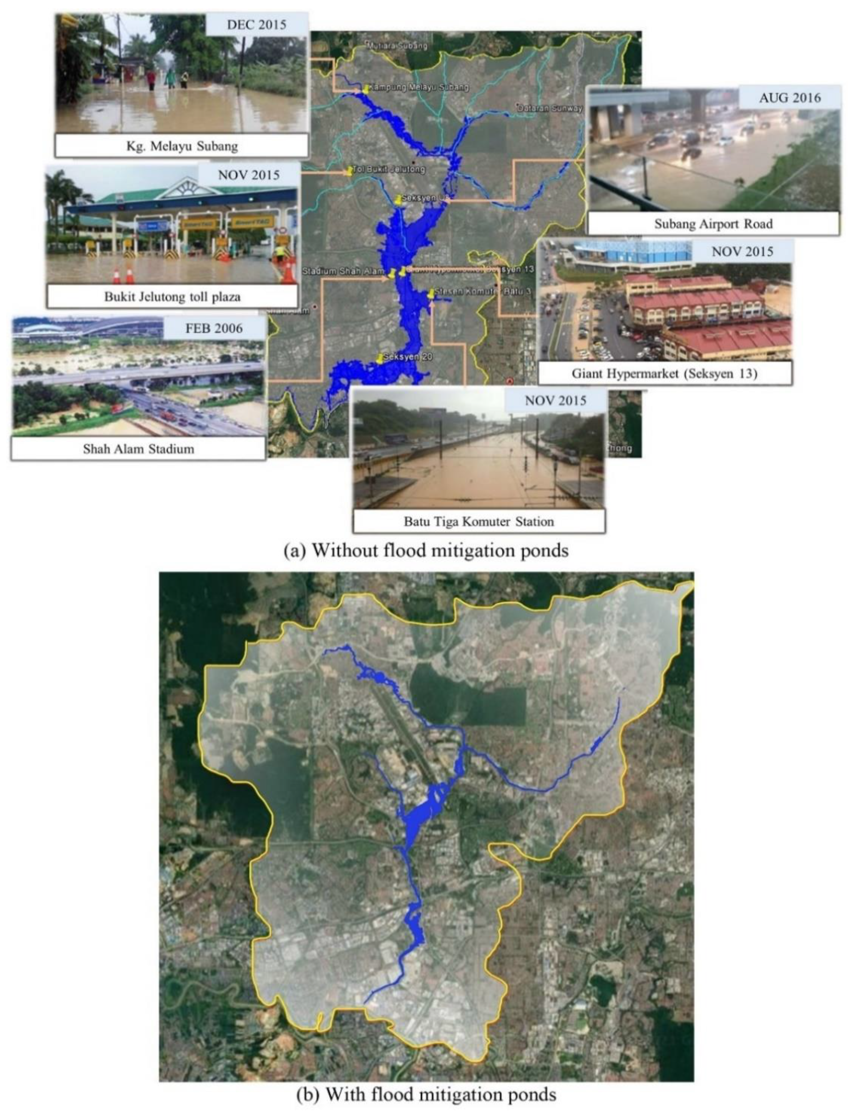
4.2. Flooding Scenarios with and without the Regional Ponds as Flood Mitigation Measure

Figure 11 shows the simulated flood inundation for the flood event with a 100-year rainfall return period. As shown in Figure 11a, low-level regions in close proximity to the main river are subjected to flooding. These areas are in accordance with the historical flood areas as in Table 1, including Kg. Melayu Subang, Seksyen 13 Shah Alam, and Batu 3 Shah Alam. In the Damansara catchment, the issue of flooding is commonly triggered by excessive rains, coupled with increased impermeable surfaces, and insufficient drainage and river capacities. As such, three major regional ponds, the Rubber Research Institute Pond, Taman Eko Ara Damansara Pond, and Saujana Pond, have been used as flood mitigation measures. For a given flood event with a 100-year return period, the extent of simulated flooded areas in the Damansara catchment were 3.61 and 12.41 km², for scenarios with and without the regional ponds, respectively (Figure 11). Therefore, these mitigation ponds (with a total area of 64 ha) worked efficiently to reduce the flood extent by 8.8 km², approximately 71% relative to the scenario without the flood mitigation measure.

4.3. Flood Hazard Map

Figure 12 and Figure 13 depict the flood hazard maps generated for the Damansara catchment in different ARIs (5, 20, 50, and 100 years) and different uniform rainfall depths (250, 350, 450, and 500 mm), respectively. From the figures, the flooded areas are displayed in four hazard categories based mainly on flood depths. The qualitative results show that an increase of ARI (from 5 years to 100 years) caused a significant rise in flood depth (Figure 12). On the other hand, an increase in uniform rainfall depths (from 250 mm to 500 mm) led to a larger extent of the flooded areas, with a higher flood depth (Figure 13).

The simulated inundation areas are then correlated with the parameters of ARIs and uniform rainfall depths, as illustrated in Figure 14. One can observe in Figure 14 that the flood inundation area linearly increased with the increasing magnitude of the rainfall events. The flood with the highest ARI (100 years) showed the largest flooded area, which covered about 3.61 km², equivalent to 1.42 times the total area inundated by the case of 2-year ARI floods (Figure 14a). On the other hand, the flood inundation area increased up to 2.62 times as the uniform rainfall depth increased from 250 mm to 500 mm (Figure 14b). This observation indicates that the effect of uniform rainfall depths was more pronounced on the extent of flooded areas.

As expected, the magnitude of flooding within a catchment is significantly affected by the amount of water discharged during a rainfall event. Furthermore, it is also attributed to the topography characteristics of the river cross-section and floodplain. As we can see from Figure 12a and Figure 13a, flooding occurs in the middle of the Damansara catchment adjoined with a low-lying floodplain, even subjected to a minor storm (flood at 5-year ARI and 250 mm rainfall depth). Flood hazard mapping plays an important role in floodplain management and acts as a basis for designing structural and non-structural measures [52]. Therefore, the flood hazard maps need to be revised periodically due to hydraulics changes and the availability of better topographic data.

5. Conclusions

In this study, hydrological−hydraulic modeling of urban floods in the Damansara catchment was performed using InfoWorks ICM, with high-resolution DTM data generated using the IFSAR technique. The methodologies and findings provided a reliable basis for the subsequent application of the proposed model, while indicating the need for a detailed analysis of land use and the role of water storage tanks. Several important conclusions are presented herein.

• The calibration and validation results confirm the reliability of the developed model, where the peak discharge is found to be accurately predicted with a maximum of 0.10% relative error.
• The work demonstrates the importance of detention ponds, where the existence of 64-ha regional ponds contributes to flood mitigation in the Damansara catchment, which has a 71% reduction in the flood extent.
• The magnitude of flooding is dependent on the flood event ARIs and uniform rainfall depths. Flood events at a high ARI cause a higher floodwater depth, whereas the effect of uniform rainfall depths is pronounced on both the flood depth and extent.
• The correlation between the parameters of ARI and uniform rainfall depth on the resulting flood inundation area is drawn, serving as references for mitigating floods in other similar tropical regions.

Floods are commonly associated with power outages [53], caused by submergence and damage to electrical generation facilities. Tenaga Nasional Berhad (TNB), as the largest electrical company in Malaysia, is concerned about the possible mitigation and protection of their assets against flooding. This study is part of a research project to develop a flood forecasting system for TNB’s asset protection in the Damansara catchment. A detailed flood hazard assessment will be included in the next study scope by overlaying TNB’s assets with the flood hazard maps developed in this study.

References

1. Ritchie, H.; Roser, M. Natural Disasters-Empirical View. Available online: https://ourworldindata.org/natural-disasters#citation (accessed on 1 July 2020).
2. IPCC. Climate Change 2014: Synthesis Report. Contribution of Working Groups I, II and III to the Fifth Assessment Report of the Intergovernmental Panel on Climate Change; Intergovernmental Panel on Climate Change: Geneva, Switzerland, 2014. [Google Scholar]
3. Asiedu, J.B. Reviewing the argument on floods in urban areas: A look at the causes. Theor. Empir. Res. Urban Manag. 2020, 15, 24–41. [Google Scholar]
4. Nath, B.; Ni-Meister, W.; Choudhury, R. Impact of urbanization on land use and land cover change in Guwahati city, India and its implication on declining groundwater level. Groundw. Sustain. Dev. 2021, 12, 100500. [Google Scholar] [CrossRef]
5. Mahmood, M.I.; Elagib, N.A.; Horn, F.; Saad, S.A. Lessons learned from Khartoum flash flood impacts: An integrated assessment. Sci. Total. Environ. 2017, 601, 1031–1045. [Google Scholar] [CrossRef] [PubMed]
6. Tshimanga, R.M.; Tshitenge, J.M.; Kabuya, P.; Alsdorf, D.; Mahe, G.; Kibukusa, G.; Lukanda, V. A regional perceptive of flood forecasting and disaster management systems for the Congo River basin. In Flood Forecasting: A Global Perspective; Academic Press: Cambridge, MA, USA, 2016; pp. 87–124. [Google Scholar]
7. Serban, P.; Askew, A. Hydrological forecasting and updating procedures. Hydrol. Water Manag. Large River Basins 1991, 201, 357–369. [Google Scholar]
8. Islam, Z. A Review on Physically Based Hydrologic Modeling; University of Alberta: Edmonton, AB, Canada, 2011. [Google Scholar]
9. Sušanj, I.; Ožanić, N.; Marović, I. Methodology for developing hydrological models based on an artificial neural network to establish an early warning system in small catchments. Adv. Meteorol. 2016, 2016, 9125219. [Google Scholar] [CrossRef] [Green Version]
10. Dawson, C.; Wilby, R. Hydrological modelling using artificial neural networks. Prog. Phys. Geogr. 2001, 25, 80–108. [Google Scholar] [CrossRef]
11. Wong, T.; Koh, X.C. Which model type is best for deterministic rainfall-runoff modelling. In Water Resources Research Progress; Nova Science Publishers: New York, NY, USA, 2008; pp. 241–260. [Google Scholar]
12. Brirhet, H.; Benaabidate, L. Comparison of two hydrological models (lumped and distributed) over a pilot area of the issen watershed in the Souss Basin, Morocco. Eur. Sci. J. 2016, 12, 347–358. [Google Scholar] [CrossRef] [Green Version]
13. Diaconu, D.C.; Costache, R.; Popa, M.C. An Overview of Flood Risk Analysis Methods. Water 2021, 13, 474. [Google Scholar] [CrossRef]
14. Craninx, M.; Hilgersom, K.; Dams, J.; Vaes, G.; Danckaert, T.; Bronders, J. Flood4castRTF: A Real-Time Urban Flood Forecasting Model. Sustainability 2021, 13, 5651. [Google Scholar] [CrossRef]
15. Costache, R.; Bao Pham, Q.; Corodescu-Roșca, E.; Cîmpianu, C.; Hong, H.; Thi Thuy Linh, N.; Ming Fai, C.; Najah Ahmed, A.; Vojtek, M.; Muhammed Pandhiani, S. Using GIS, remote sensing, and machine learning to highlight the correlation between the land-use/land-cover changes and flash-flood potential. Remote Sens. 2020, 12, 1422. [Google Scholar] [CrossRef]
16. Abdelkarim, A.; Al-Alola, S.S.; Alogayell, H.M.; Mohamed, S.A.; Alkadi, I.I.; Youssef, I.Y. Mapping of GIS-Flood Hazard Using the Geomorphometric-Hazard Model: Case Study of the Al-Shamal Train Pathway in the City of Qurayyat, Kingdom of Saudi Arabia. Geosciences 2020, 10, 333. [Google Scholar] [CrossRef]
17. Anees, M.T.; Abdullah, K.; Nawawi, M.N.; ARahman, N.N.; Ismail, A.Z.; Syakir, M.I.; Abdul Kadir, M.O. Prioritization of Flood Vulnerability Zones Using Remote Sensing and GIS for Hydrological Modelling. Irrig. Drain. 2019, 68, 176–190. [Google Scholar] [CrossRef]
18. Peng, H.-Q.; Liu, Y.; Wang, H.-W.; Ma, L.-M. Assessment of the service performance of drainage system and transformation of pipeline network based on urban combined sewer system model. Environ. Sci. Pollut. Res. 2015, 22, 15712–15721. [Google Scholar] [CrossRef]
19. Kuok, K.K.; Chen, E.; Chiu, P.C. Integration of IR4. 0 with Geospacial SuperMap GIS and InfoWorks ICM. Solid State Technol. 2020, 63, 21651–21662. [Google Scholar]
20. Biswas, R.R. Modelling seismic effects on a sewer network using Infoworks ICM. Indian J. Sci. Technol. 2017, 10, 1–9. [Google Scholar] [CrossRef] [Green Version]
21. Sheng, J.G.; Dan, Y.D.; Liu, C.S.; Ma, L.M. Study of Simulation in Storm Sewer System of Zhenjiang Urban by Infoworks ICM Model. Appl. Mech. Mater. 2012, 193, 683–686. [Google Scholar] [CrossRef]
22. Yang, H.; Tong, X.; Gou, D. Study on the waterlogging operation effects of InfoWorks ICM dispatching strategies. E3S Web Conf. 2021, 228, 01009. [Google Scholar] [CrossRef]
23. Sameer, M.; Rustum, R. Studying the impact of construction dewatering discharges to the urban storm drainage network (s) of Doha city using infoworks integrated catchment modeling (ICM). MATEC Web Conf. 2017, 120, 08010. [Google Scholar] [CrossRef] [Green Version]
24. Musa, S.; Adnan, M.; Ahmad, N.; Ayob, S. Flood Water Level Mapping and Prediction Due to Dam Failures. IOP Conference Series: Materials Science and Engineering 2016, 136, 012084. [Google Scholar] [CrossRef] [Green Version]
25. Muhadi, N.A.; Abdullah, A.F.; Vojinovic, Z. Estimating agricultural losses using flood modeling for rural area. MATEC Web Conf. 2017, 103, 04009. [Google Scholar] [CrossRef] [Green Version]
26. Leitao, J.; Simoes, N.; Pina, R.D.; Ochoa-Rodriguez, S.; Onof, C.; Sa Marques, A. Stochastic evaluation of the impact of sewer inlets’ hydraulic capacity on urban pluvial flooding. Stoch. Environ. Res. Risk Assess. 2017, 31, 1907–1922. [Google Scholar] [CrossRef]
27. Cheng, T.; Xu, Z.; Hong, S.; Song, S. Flood risk zoning by using 2D hydrodynamic modeling: A case study in Jinan City. Math. Probl. Eng. 2017, 2017. [Google Scholar] [CrossRef] [Green Version]
28. Besseling, L. Validity Assessment of D-Hydro Urban: Comparing D-Hydro with Infoworks ICM in a Beverwijk Sewer Modelling Study. Bachelor’s thesis, University of Twente, Enschede, The Netherlands, 2020. [Google Scholar]
29. Yushmah, M.; Bracken, L.; Zuriatunfadzliah, S.; Norhaslina, H.; Melasutra, M.; Amirhosein, G.; Sumiliana, S.; Shereen Farisha, A. Understanding urban flood vulnerability and resilience: A case study of Kuantan, Pahang, Malaysia. Nat. Hazards 2020, 101, 551–571. [Google Scholar] [CrossRef] [Green Version]
30. DID. National Register of River Basins: Registry of River Basin; Department of Irrigation and Drainage Malaysia: Kuala Lumpur, Malaysia, 2003.
31. DID. Ringkasan Laporan Banjir Tahunan Bagi Tahun 2014/2015; Department of Irrigation and Drainage Malaysia: Kuala Lumpur, Malaysia, 2015.
32. DID. Ringkasan Laporan Banjir Tahunan Bagi Tahun 2015/2016; Department of Irrigation and Drainage Malaysia: Kuala Lumpur, Malaysia, 2016.
33. DID. Ringkasan Laporan Banjir Tahunan Bagi Tahun 2016/2017; Department of Irrigation and Drainage Malaysia: Kuala Lumpur, Malaysia, 2017.
34. Godunov, S.K. A difference scheme for numerical solution of discontinuous solution of hydrodynamic equations. Mat. Sb. 1959, 47, 271–306. [Google Scholar]
35. Alcrudo, F.; Mulet-Marti, J. Urban inundation models based upon the Shallow Water equations. Numerical and practical issues. In Proceedings of the Finite Volumes for Complex Applications IV. Problems and Perspectives, Marrakech, Morocco, 4–8 July 2005; pp. 1–12. [Google Scholar]
36. Innovyze. 2D Hydraulic Theory. Available online: https://www.innovyze.com/en-us/blog/2d-hydraulic-theory (accessed on 3 July 2021).
37. Moore, R. The PDM rainfall-runoff model. Hydrol. Earth Syst. Sci. 2007, 11, 483–499. [Google Scholar] [CrossRef]
38. Akter, T.; Quevauviller, P.; Eisenreich, S.J.; Vaes, G. Impacts of climate and land use changes on flood risk management for the Schijn River, Belgium. Environ. Sci. Policy 2018, 89, 163–175. [Google Scholar] [CrossRef]
39. Yaduvanshi, A.; Srivastava, P.; Worqlul, A.W.; Sinha, A.K. Uncertainty in a Lumped and a Semi-Distributed Model for Discharge Prediction in Ghatshila Catchment. Water 2018, 10, 381. [Google Scholar] [CrossRef] [Green Version]
40. Jian, J.; Ryu, D.; Costelloe, J.F.; Su, C.-H. Towards hydrological model calibration using river level measurements. J. Hydrol. Reg. Stud. 2017, 10, 95–109. [Google Scholar] [CrossRef]
41. Azad, W.H.; Sidek, L.M.; Basri, H.; Fai, C.M.; Saidin, S.; Hassan, A.J. 2 dimensional hydrodynamic flood routing analysis on flood forecasting modelling for Kelantan River Basin. MATEC Web Conf. 2017, 87, 01016. [Google Scholar] [CrossRef] [Green Version]
42. DID. Urban Stormwater Management Manual for Malaysia; Department of Irrigation and Drainage Malaysia: Kuala Lumpur, Malaysia, 2012.
43. Samuels, P. Cross section location in one-dimensional models. In Proceedings of the International Conference on River Flood Hydraulics, Wallingford, UK, 17–20 September 1990; pp. 339–350. [Google Scholar]
44. Ackers, J. Hydraulic analysis and design. In Fluvial Design Guide; Environment Agency: Bristol, UK, 2010. [Google Scholar]
45. Ogania, J.; Puno, G.; Alivio, M.; Taylaran, J. Effect of digital elevation model’s resolution in producing flood hazard maps. Glob. J. Environ. Sci. Manag. 2019, 5, 95–106. [Google Scholar]
46. Mercer, B. Comparing LIDAR and IFSAR: What can you expect. In Proceedings of the Photogrammetric Week, Stuttgart, Germany, 5–9 September 2001; pp. 2–10. [Google Scholar]
47. Shewchuk, J.R. Triangle: Engineering a 2D quality mesh generator and Delaunay triangulator. Lect. Notes Comput. Sci. 1996, 1148, 203–222. [Google Scholar]
48. Kirpich, Z. Time of concentration of small agricultural watersheds. Civ. Eng. 1940, 10, 362. [Google Scholar]
49. Zhou, Q. A review of sustainable urban drainage systems considering the climate change and urbanization impacts. Water 2014, 6, 976–992. [Google Scholar] [CrossRef]
50. Sidek, L.M.; Basri, H.; Thiruchelvam, S.; Chow, M.F.; Zawawi, M.H.; Hossain, M.S. Research on Impacts of Floods on TNBD’s PMU/PPU/SSU/PE and the Proposed Mitigation Measures; Universiti Tenaga Nasional: Selangor, Malaysia, 2016. [Google Scholar]
51. Gumbel, E.J. Statistics of Extremes; Columbia University Press: New York, NY, USA, 1958. [Google Scholar]
52. Alaghmand, S.; Abdullah, R.; Abustan, I.; Vosoogh, B. GIS-based river flood hazard mapping in urban area (a case study in Kayu Ara River Basin, Malaysia). Int. J. Eng. Technol. 2010, 2, 488–500. [Google Scholar]
53. Karagiannis, G.M.; Chondrogiannis, S.; Krausmann, E.; Turksezer, Z.I. Power Grid Recovery after Natural Hazard Impact; European Commission: Luxembourg, 2017. [Google Scholar]
Figure 1. (a) Damansara catchment with the distribution of meteorological stations; (b) Damansara River and its attributes within the catchment.
Sustainability 13 10259 g001
Figure 2. Major land uses in the Damansara catchment (obtained from Department of Town and Country Planning, Malaysia).
Sustainability 13 10259 g002
Figure 3. Simplified process for flood hazard map development.
Sustainability 13 10259 g003
Figure 4. Delineation of sub-catchments for the Damansara catchment (number of sub-catchments = 64).
Sustainability 13 10259 g004
Figure 5. Example of a cross-sectional profile of a river channel within the Damansara catchment.
Sustainability 13 10259 g005
Figure 6. Digital terrain model for the Damansara catchment.
Sustainability 13 10259 g006
Figure 7. (a) 1D river and 2D floodplain representations for the Damansara catchment (number of 2D elements = 5826; area covered = 68.70 km2); (b) 3D view of the Damansara catchment.
Sustainability 13 10259 g007
Figure 8. Calibration point at the Water Level Station at TTDI Jaya (no. 3015490).
Sustainability 13 10259 g008
Figure 9. Location of ponds modeled in Infoworks ICM.
Sustainability 13 10259 g009
Figure 10. Comparison of observed and modeled water level time series during (a) calibration and (b) validation.
Sustainability 13 10259 g010
Figure 11. Flood inundation for a flood event with a 100-year rainfall return period.
Sustainability 13 10259 g011
Figure 12. Flood hazard maps for several ARIs for the Damansara catchment.
Sustainability 13 10259 g012
Figure 13. Flood hazard maps for several uniform rainfall depths for the Damansara catchment.
Sustainability 13 10259 g013
Figure 14. Correlation between (a) ARI and flood inundation area, and (b) uniform rainfall depth and flood inundation area.
Sustainability 13 10259 g014