Article

Beef Cattle Price and Production Patterns in Relation to Drought in New Mexico

by
Ashraf J. Zaied
1,
Hatim M. E. Geli
1,2,*,
Andres F. Cibils
1,
Mohammed N. Sawalhah
3,
Jerry L. Holechek
1,
Charlotte C. Gard
4,
Saleh A. Idhirij
5,
Melakeneh G. Gedefaw
6 and
Greg L. Torell
5
1
Department of Animal and Range Sciences, New Mexico State University, Las Cruces, NM 88003, USA
2
New Mexico Water Resources Research Institute, New Mexico State University, Las Cruces, NM 88003, USA
3
Department of Lands Management and Environment, Prince Al-Hasan Bin Talal Faculty for Natural Resources and Environment, The Hashemite University, Zarqa 13133, Jordan
4
Department of Economics, Applied Statistics & International Business, New Mexico State University, Las Cruces, NM 88003, USA
5
Department of Agricultural Economics and Agricultural Business, New Mexico State University, Las Cruces, NM 88003, USA
6
Water Science and Management Program, New Mexico State University, Las Cruces, NM 88003, USA
*
Author to whom correspondence should be addressed.
Sustainability 2021, 13(18), 10420; https://doi.org/10.3390/su131810420
Submission received: 13 August 2021 / Revised: 11 September 2021 / Accepted: 13 September 2021 / Published: 18 September 2021
(This article belongs to the Special Issue Sustaining Rangeland Ecosystems for the Benefit of Society)

Abstract

:
Understanding the fluctuations in monthly and annual cattle prices plays a key role in supporting the sustainability of New Mexico’s (NM’s), United States (US), beef cattle industry under variable environmental conditions. The goal of this study was to provide an improved understanding of NM’s beef cattle production systems in terms of prices and production patterns and related drought impacts. The main objectives were to evaluate monthly and annual prices patterns for heifers and steers (cattle) and calves, the relationships between annual cattle prices and inventory and drought, and the effects of drought on ranch net return. Drought events were assessed using the Self-Calibrated Palmer Drought Severity Index (SC-PDSI). The generalized autoregressive conditional heteroscedasticity models and their exponential version were used to investigate the effects of drought and cattle supply on cattle prices, and the effects of drought on ranch net return. Spectral analysis and timeseries decomposition were used to identify the cycles of the annual price and numbers of cattle and calf. Coherence analysis was used to examine the relationships between inventory of cattle classes and drought. The results indicated that prices of cattle and calf usually drop in October through January and peak in April. The inventory of replacement heifers and steers were negatively related to cattle prices, while the inventory of calves was positively related to calf prices. Cattle and calf prices showed negative linear relationships with droughts. Annual cattle and calf prices showed 6- and 10-year cycles, while their inventory showed 6- and 8- year cycles, respectively. Our finding suggested that a rancher can still earn some net return when drought falls within the “Abnormally Dry” category of the US Drought Monitor. However, a rancher with a large herd or ranch size can endure drought more than a rancher with a medium herd or ranch size and reach the breakeven point. Specifically, the net return ($/head) is expected to increase (or decrease) by $62.29, $60.51, and $64.07 per head if the SC-PDSI increase (or decrease) by one unit in all large and medium ranch sizes, respectively. The effects of drought on ranch net return that we identified need further improvements using additional data. Due to NM’s location and the diversity of its rangeland, understanding the response of cattle prices to drought and beef cattle supply based on these findings can be used to help NM’s ranchers and those in other similar regions make informed ranch management decisions. These findings can also support the development of improved understanding of beef cattle production systems regionally.

1. Introduction

Providing improved qualitative and quantitative descriptions of beef cattle production systems is key to enhancing the resilience to drought and socioeconomic impacts [1,2,3,4]. This analysis was conducted within the context of developing an integrated model to better represent food, energy, and water systems. Increased frequency and duration of drought events specially in arid and semi-arid regions such as New Mexico (NM) in the southwestern United States of America (USA) can negatively affect beef cattle production systems that depend mainly on rangelands [3,5,6,7]. Due to climate change, many areas in southwestern US are expected to experience even more extreme drought conditions in the future as indicated by the World Research Institute (WRI) [8]; thus, impacting the availability of suitable forage to support beef cattle production. On the other hand, a more than 50% increase in demand for meat including beef during the next 30 years is expected due to population growth [9]. These competing factors put additional pressure on rangeland beef cattle production systems, the environment, and their economic feasibility. These systems are frequently the main source of livelihood for many western US farmers and ranchers.
Understanding monthly and annual cattle prices patterns and the potential interaction between cattle prices, drought, and economic variables can help ranchers operate successful businesses by allowing them to make effective management and marketing decisions. As indicated by Anderson et al. [10], “A seasonal pattern is a regularly repeating pattern that is completed once every twelve months, while a cycle is a pattern that repeats itself regularly over a period of years”. These patterns and cycles of prices can be affected by the environment and market requirements [11].
Beef demand in the US has fallen from its peak in the 1980s by nearly 4.5 kg of beef products consumed per capita, while inflation-adjusted prices fell by over 30% over the same time period. Demand for beef has stabilized in recent years, and export markets are an increasingly important component of beef demand, and the largest area of potential growth for this sector. However, demand for beef is sensitive to macroeconomic conditions. The own-price elasticity for beef products is −0.61, meaning that the quantity of beef demanded falls by 0.61% for every 1% increase in beef prices. Simultaneously, beef demand is sensitive to consumer incomes, increasing 0.9% for every 1% increase in consumer disposable income [12]. Consumers have been shown to be concerned about the sustainability impacts and health impacts of beef products, and the animal welfare implications of production systems [12,13,14].
On the supply side, producers have heterogenous expectations of the prices they will be able to fetch at final sale of their cattle. Nearly half of cattle growers behave ‘naïvely’, assuming that their final sale price will be the same or close to the most recent observed market price. This is in contrast to only 18% of beef producers using rational expectations (those that use forward-looking estimations based on data) when estimating final sale prices, indicating that the formation of rational expectations based on data and analysis is a costly endeavor that nearly half of producers do not see a net benefit in performing [15]. Work that sheds light on cattle price dynamics can provide information that reduces these costs and can help producers in profitable and sustainable decision making.
The cattle industry is one of the pillars of the state of NM’s economy and contributes to ensure food security in the USA. More than one third of NM’s total land is considered cropland and ranches, and most of this land is employed for grazing purposes [16]. In 2018, the total agricultural receipts were about $2,919,467,000. In that year, cattle and calves accounted for 31.4% ($919,041,000) of the state’s total agricultural receipts [17]. In addition, NM’s beef cattle play an important role in meeting the demand for red meat in other states, as they are usually exported to different markets in Colorado, Missouri, Texas, and California [16].
Monthly and annual variations in cattle prices (on a live weights basis) have been a prevalent trait of cattle marketing in the USA [6,18]. For instance, in Midwestern USA, monthly prices of feeder steers (weighing from 226.7 to 272 kg) show an increased trend between January and August with a declining trend between October and December. However, prices for steers weighing between 317.5 to 362.8 kg can reach a peak value in late summer and then drop gradually to reach the lowest price in January [18]. Regarding the cattle price cycles in the USA between 1945 and 1995, they averaged three years of increase followed by two years of decline for both cattle and calves [19]. Another study indicated that the cattle price cycles were characterized by 6–7 years of increase then followed by 3–5 years of decline [20].
Cattle prices can be affected by supply and demand principles. Ranchers often increase their herd size when cattle prices are high and sell off it when prices drop [10]. However, an increase in cattle inventory can lead to a decline in cattle prices due to increased supply that can result in operation liquidations, which continue until prices climb again [19]. In addition, increased market demand for beef can result in reducing the current supply due to the fact that calves are held back to gain more weight, or they are retained for reproduction purposes to increase the cow herd size and increase future production [21,22]. In fact, there is a time lag in the response of cattle prices to an increase in herd size due to the biological nature of beef cattle production. Heifers that are withheld for increasing the herd size cannot contribute to increase beef cattle production until they are at least three years old [10]. However, when future demand is expected to decline, current supply increases. In this case, calf prices decline promptly to ensure a high level of consumption and reduction of herd size [22].
Research literature regarding optimal management strategies for beef cattle production systems during prolonged periods of drought indicate that a liquidation of herds one of the best strategies to follow [7,23,24], even though it can lead to a decline in prices for all cattle classes [19]. Reducing the stocking rate to less than the average during two years of drought is the best strategy for profitability in the long term [25]. The purpose of cutting stocking rates is to preserve the forage base to feed the remaining herd—this approach is considered the best and most effective management plan during drought [26]. This approach also allows ranchers to reduce the use of feed supplements whose prices usually increase during droughts, leading to an increase in ranching costs [7,23].
In New Mexico, the fluctuations in cattle prices can partly be attributed to drought [1,6]. Droughts are commonly associated with low cattle prices, and this phenomenon occurs in a cyclic manner every 40 years and continues for 4–6 years [7]. Between 1984 and 1993, the precipitation was above average and resulted in an increase in forage production, that coincided with an increase in cattle prices by about 41–53%, compared to those of 1986 [6]. However, the 1994 drought resulted in a decline in forage production as well as cattle prices that was estimated to be 25% of the peak price during the 1992–1994 period [6]. It has been shown that drought can reduce forage production by more than 50% in New Mexico, compared to the pre-drought conditions [27,28]. In such situations, the best strategy for NM’s ranchers would be to reduce the herd size by about 50% [23]. Moreover, a study by Gedefaw et al. [29] indicated that there have been regional rangeland degradation over New Mexico that has been considered as permanent change—in which case the rancher would need to adjust their management practices to these new conditions.
The goal of this study was to provide an improved understanding of New Mexico’s beef cattle production systems in terms of prices and production patterns and the corresponding impacts from drought. Such understanding can provide NM ranchers with the means to develop well informed rangeland management decisions. Further, we sought to inform the development of an integrated food-energy-water systems model as depicted in Yadav et al. [1]. This analysis was based on the hypothesis that drought will lead to increased beef cattle sale and consequently decreased beef cattle prices and ranch net return in arid to semi-arid regions like New Mexico. The objectives of this study were to evaluate (1) monthly and annual prices patterns for heifers and steers (cattle) and calves, (2) the relationships between annual cattle prices and inventory and drought; and (3) the effects of drought on ranch net return.

2. Methodology

2.1. Study Area

The study focused on cattle prices averaged over the entire state of New Mexico, which is located in southwestern USA (31°20′ N to 37° N) and (103° W to 109°3′ W). Most of NM’s precipitation falls during the summer months of July and August, with little amounts in January. The mean annual precipitation in the southern desert and the Rio Grande and San Juan valleys is less than 254 mm, while it reaches 508 mm at the higher elevations. The mean annual temperatures vary from 17.7 °C in southeast to 4.4 °C in the high mountains and valleys of the north. The maximum temperatures range from 32.2 °C to 21.1 °C in lower and high elevations, respectively [30]. Annual evaporation rate is more than 250 mm [31].

2.2. Data

The study used 51 years (1960–2010) of data that include cattle and calf numbers, cattle and calf prices, and the Self-Calibrated Palmer Drought Severity Index (SC-PDSI) [5]. Cattle and calf inventory as well as mean monthly and annual prices of heifers, steers, and calf ($/45.4 kg) were obtained from the United States Department of Agriculture-National Agricultural Statistics Service (USDA-NASS) [17]. The SC-PDSI data was retrieved from Western Regional Climate Center [32]. The Consumer Price Index (CPI) was obtained from Federal Reserve Economic Data (FRED) [33].
Calf’s numbers and prices (live weights) as reported by the USDA are those of animals that are less than one year old and weigh less than 226.7 kg. Cattle prices and numbers used in this study refer to those of cattle that are more than one year old and weigh more than 226.7 kg, including heifers for replacement and heifers (exclude replacement) and steers.
Estimates of costs and returns of some ranches in New Mexico were obtained from New Mexico State University (https://aces.nmsu.edu/cropcosts/index.html, accessed on 20 May 2021) [34]. These estimates were based on survey data collected over five different regions in the state (i.e., central, southwest, southeast, northeast, northwest). Ranch budgets were evaluated based on four ranch size categories that include small, medium, large, and extra-large represented by herd sizes of less 100, 100–200, 200–400, and more than 400, respectively. For consistency, the data from medium and large ranch sizes were used in this analysis as not all regions have all the ranch size categories. These datasets were available for the 2010–2019 period.

2.3. Data Processing and Analysis

All prices were adjusted for inflation to reflect 2010 dollars using the CPI. Monthly price patterns were determined based on prices of cattle and calves for each month over the 51-year period (1960–2010) [18]. Regression analysis was conducted to determine the relationships between cattle and calf prices and the numbers of cattle—including replacement heifers, heifers (excluding replacement) and steers, and calves—and drought. Autocorrelation and heteroscedasticity were diagnosed in all data by using Durbin–Watson statistics (1st through 10th order) and Portmanteau tests and Engle Lagrange multiplier tests (12 lag windows), respectively. Therefore, the exponential version of generalized autoregressive conditional heteroscedasticity (EGARCH) model was used [35] with backward elimination used to remove insignificant autoregressive terms. Proc AUTOREG available in the SAS software [36] was utilized for this purpose.
The length of the cycles of cattle and calf prices, cattle and calf numbers, and drought were determined using spectral analysis available in the SPSS software [37]. Changes in cycles of annual cattle and calf prices, cattle and calf numbers, and drought were determined using the seasonal adjustment function available in the EViews software [38] that allows the decomposition of the timeseries of these variables into “trend”, “seasonal”, and “random” components. Wavelet coherence available in the R statistical software [39] was used to examine the relationships between numbers of all cattle classes and the SC-PDSI. Statistical significance was determined based on an alpha level of 0.05.
To evaluate the effect of drought on ranch return, multilinear regressions between drought and net ranch return for the data between 2010 and 2019 were assessed. Different drought severity scenarios were used to evaluate the corresponding ranch net return. Ranges of drought severity was accounted for by changing the SC-PDSI values to reflect the five drought categories as identified by the United States Drought Monitor (i.e., D0 to D4) [40].

3. Results and Discussion

3.1. Monthly Price Patterns

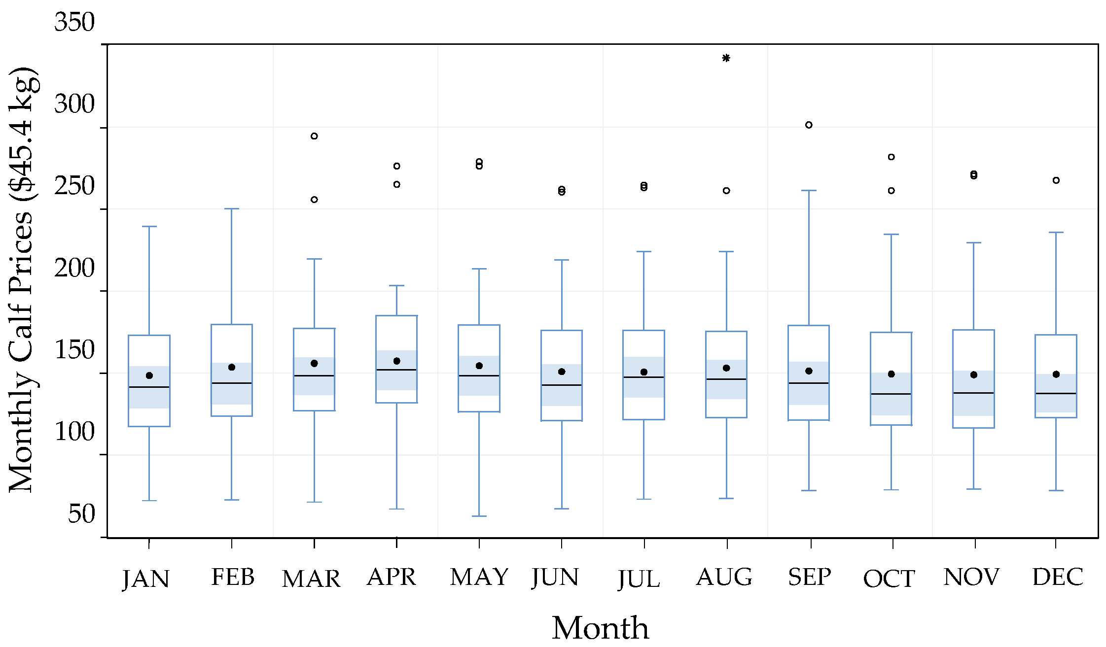
A summary of the average monthly cattle and calf price patterns is shown in Table 1. The prices did not show significant monthly variation during the 1960–2010 period. Cattle prices increased from February through May and decreased in June and July, then increased again from August to October. The lowest prices were observed in November and December with a 6% decline from the April peak price (Figure 1). However, calf prices did not show notable differences between October, November, and December, but they showed a notable increase from February through April, then dropped in June and July and increased again in August. The lowest observed prices were in January, which were about 7.6% below the peak prices that were recorded in April (Figure 2).
The declining trend in prices of cattle and calf in January, November, and December can be attributed to the fact that plant dormancy limits rangeland forage production [31,41]. Thus, ranchers may not be able to keep more animals without accruing additional ranching expenses (due to increased use of supplemental feeds) and, therefore, some ranchers prefer to reduce the size of their herds in order to avoid using feed supplementation [23]. Also, weaning of calves occurs during these months, so a considerable number of calves are ready to be sold during this time of the year. These factors may cause an increase in beef supply, resulting in a decline in cattle and calf prices. However, increased cattle and calf prices in March, April, and May might be a result of a rapid rate of plant growth due to favorable conditions—temperature and soil moisture—allowing to provide increased and adequate amounts of rangeland forage [31]. As a result, ranchers are able to keep additional numbers of cattle longer [23], a practice that can lead to a decline in beef supply, which, in turn, can cause an increase in cattle and calf prices [41].
Figure 2 shows an outlier in August prices that was due to a significant increase in beef cattle prices in 1973. This outlier can partly be attributed to an increase in rangeland forage production by up to 83% compared to that of the years prior to 1973 [17], which may have been enhance by sever wet conditions, as the SC-PDSI was about 0.03 [32]. By checking the climate data for the 1973 from the Western Regional Climate Center, it was noticed that the mean annual temperature was relatively low (~11 °C), which is below the long-term average while the precipitation was about 321 mm (also below the long-term average). These conditions may have allowed to maintain adequate soil moisture for vegetation growth and reduce soil evaporation.

3.2. Annual Price Cycle

Annual prices and percentage of change in prices for the different cattle classes in New Mexico during the five decades of the 1960–2010 period are shown in Table 2. The highest negative change in cattle prices was observed during the second decade, in 1974, which was estimated to be about 27% lower than the 1973 prices. The highest positive change in cattle prices was in the third decade in 1997 and it was estimated to be about 26% higher than the 1996 prices. The range of decrease in cattle prices for all decades was different, and it was 2.6–28.5, 3–60.2, 4.3–53.7, 3.3–15.4, and 0.6–9.2 $/45.4 kg for the 1960s, 1970s, 1980s, 1990s, and 2000s, respectively. The highest negative change in calf prices was observed also in the second decade in 1974, which was about 50% lower than the 1973 prices, while the highest positive change was in 1998 and it was about 42% higher than the 1997 prices. The range of decrease in calf prices for all decades also showed some variability, and it was 4.7–35.2, 25.6–136.9, 7.9–31.4, 18.3–25, and 7.8–12.2 $/45.4 kg in the first to the last decade, respectively (Table 2).
The sharp negative change in cattle and calf prices in 1974 can be attributed to herd liquidation [6,42], caused by the drought event that occurred in 1974 that led to decrease in rangeland forage production to 60%, compared to the pre-drought period [28]. Another possible explanation for this sharp decline in prices can be attributed the fact that 1973 was relatively a very wet year (as shown in Section 3.4). Such wet conditions can result in extra feed (rangeland forage) supply that could have encouraged the ranchers to keep or breed more animals—resulting in increased cattle and calf numbers in the following year (i.e., 1974). Thus, the increased number of animals combined with the drought conditions in 1974 may have resulted in the observed sharp drop in prices. The highest positive change in cattle prices in 1997 can be attributed to wet condition, resulting in more rangeland forage production. In this case, ranchers can opt to retain their cattle [23]; as a result, cattle prices increase.
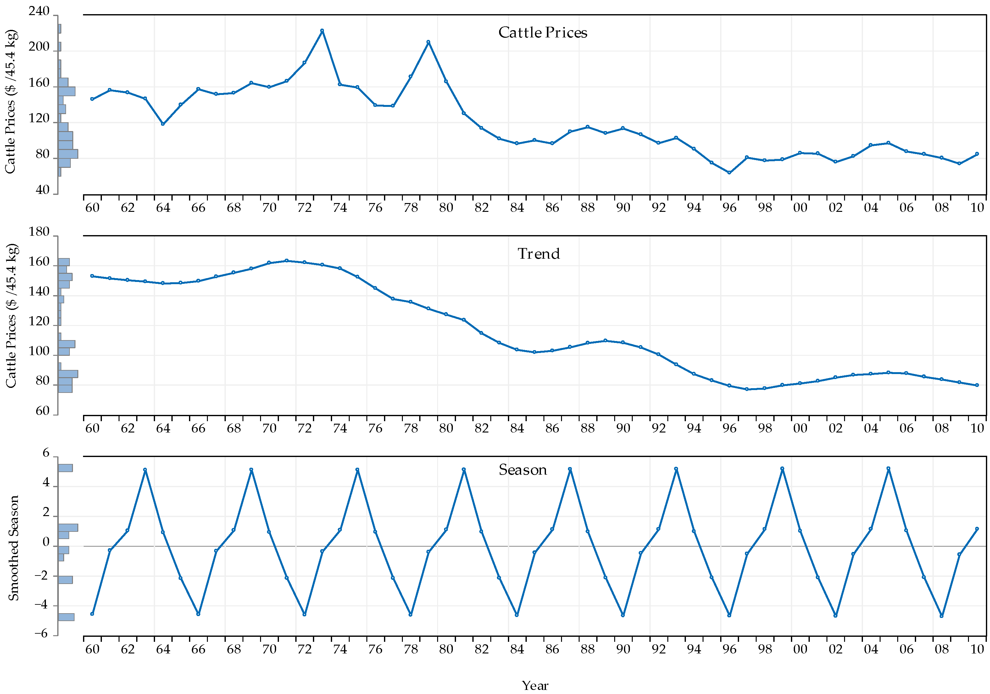
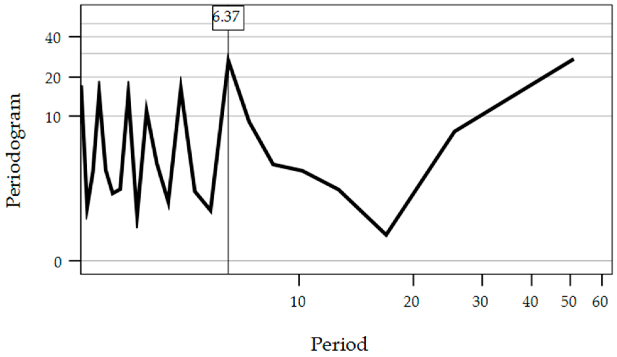
Based on the spectral analysis, which allowed to identify periodic (repeated) signals in the price timeseries, the length of the cycles (seasonality) of cattle and calf prices was found to be about 6 and 10 years, respectively (Figure 3). The length of the price cycle for cattle and calves were used to decompose their timeseries as shown in Figure 4 and Figure 5. The decomposed timeseries showed a clear declining trend in prices since the 1960s. Moreover, the seasonal pattern of prices indicated that, on average, cattle prices in each cycle had three years of increase followed by three years of decline, whereas calf prices in each cycle started decreasing from the second year through the seventh year and then showed an increase from the eighth through tenth year (Figure 4 and Figure 5).
The cycles of cattle inventory and prices are important characteristics of cattle business that need to be properly understood to better manage beef production systems. An improved knowledge of these cycles can play an important role in terms of developing informed long-term planning [10]. Holechek [6] reported that cattle prices cycle experience 6–7 years of an increase followed by 3–5 years of decline. In another study that used data for the period between 1945–1995, it was indicated that calf and cattle prices cycles experienced three years of increase followed by two years of decline [19]. However, these previous findings did not agree with those of this analysis as they were based on qualitative not quantitative statistical analysis. Another study that was conducted using data from three different countries in South America that include Brazil Chile, and Uruguay indicated that the cattle price cycle was about seven years, which falls within the same range of the identified cycle in this study [43]. The obtained cycles are in agreement with the biological aspects of beef cattle production system as the cow-calf production systems can experience long production time lags [44], due to the fact of the nine months of gestation and another six to nine months are needed until calves are ready to be sold.

3.3. Production and Drought Cycles

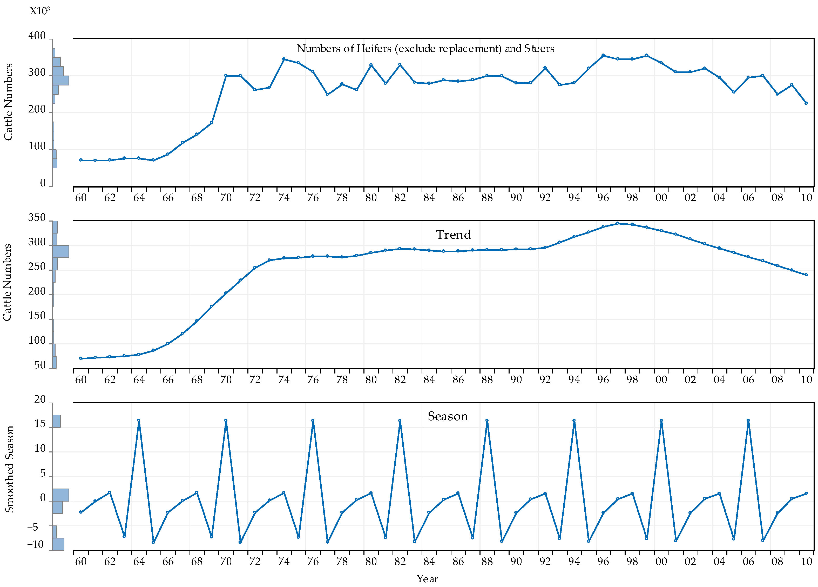
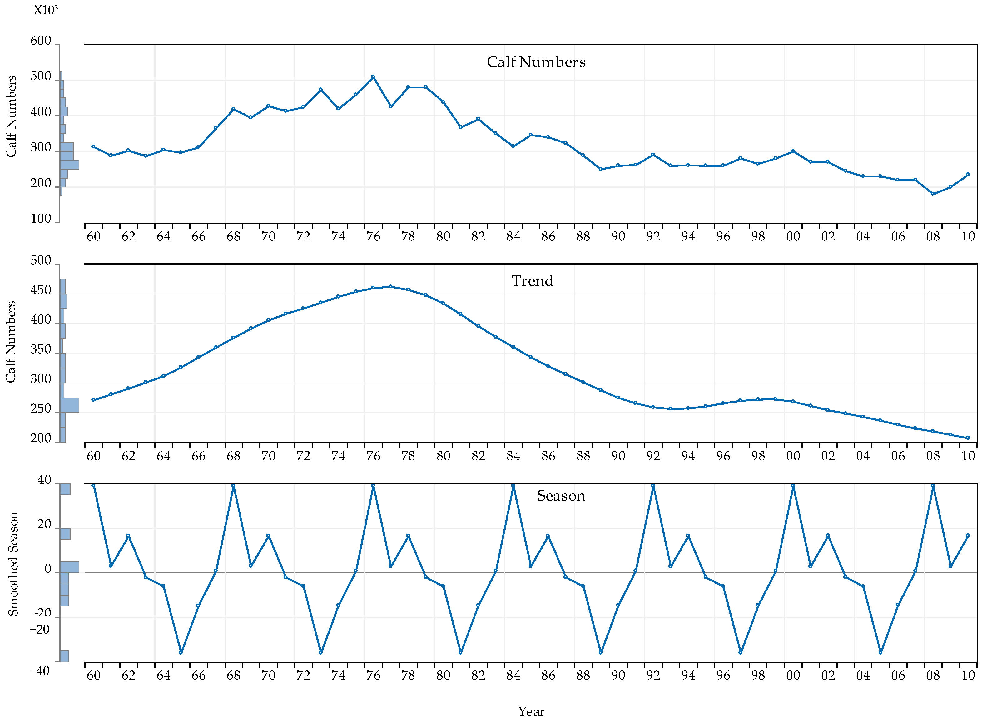
The spectral analysis was used to identify cycle in cattle and calf numbers. It was found that the lengths of cattle and calf numbers’ cycles were about six and eight years, respectively (Figure 6). The identified cycles were used to decompose their timeseries to identify their seasonality and trend. It was found that each cattle’s inventory cycle increased from the first year through the third year then declined in the fourth year followed by a sharp increase in the fifth year and declined again in the sixth year (Figure 7). However, the calf inventory cycle showed three years of increase followed by five years of decline (Figure 8). A previous study by Anderson et al. [10] showed that cattle numbers had a cyclic behavior that can be characterized by three to eight years of increase followed by three to eight years of decrease—indicating a different finding compared to this study. It was also observed that cattle (replacement heifers exclude, steers) numbers showed an increasing trend between 1960 and 1996, while a declining trend has been shown since 1999. In 2010, the decline was about 31%, compared to the peak of the 1996 (Figure 7). Calf numbers showed an increasing trend between 1960 and 1976. However, calf numbers have shown a declining trend since 1980, and in 2010 the decline was about 53%, compared to the peak in 1976 (Figure 8).
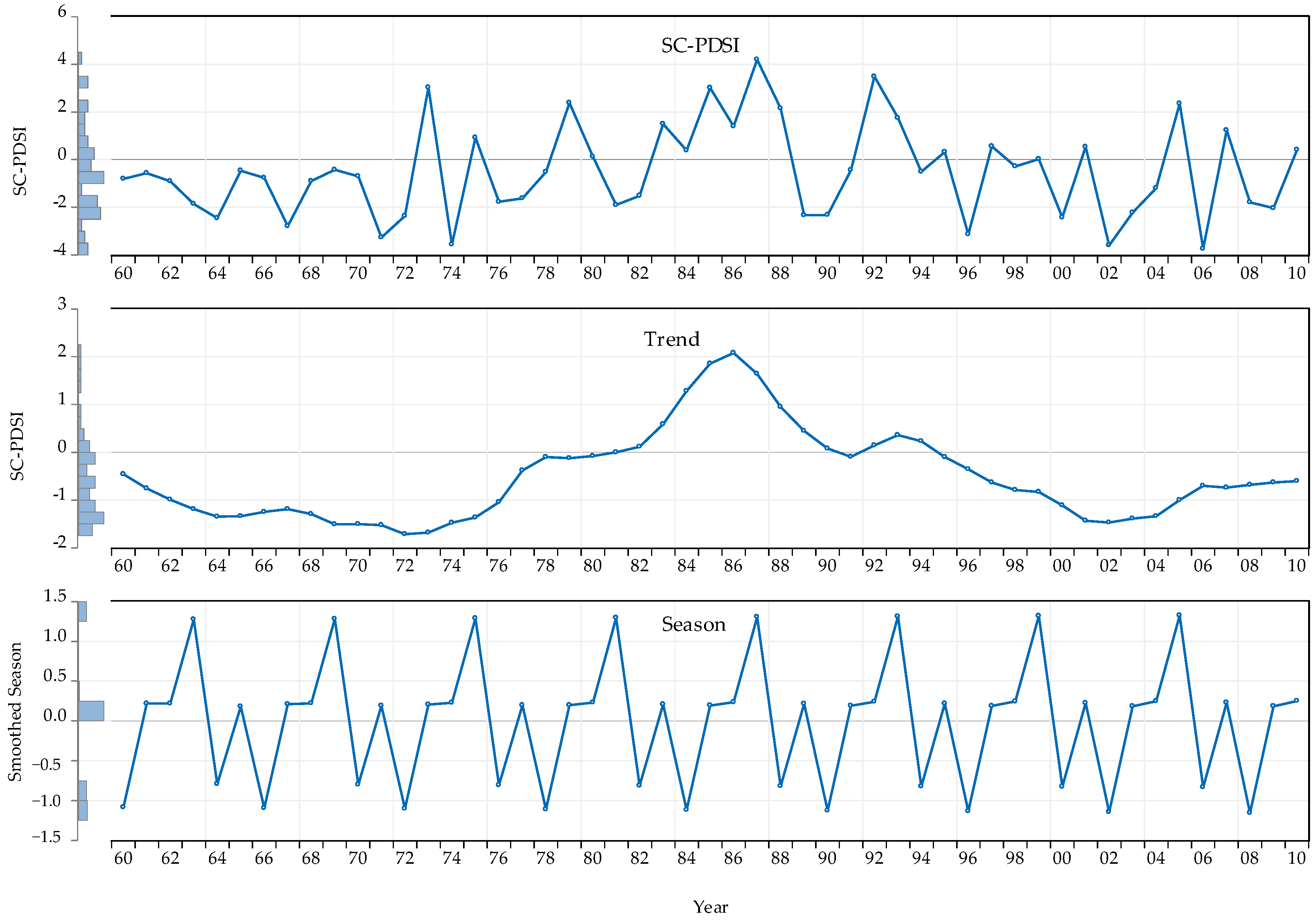
Similarly, the spectral analysis indicated that the length of SC-PDSI cycle was six years (Figure 9). In each cycle, SC-PDSI was very low in the first year and then it increased from the second year through the fourth year followed by sharp decline in the fifth year and then increased again in the sixth year (Figure 10). This may indicate that there were four wet years and two dry years in each cycle. In addition, the length of SC-PDSI cycle and the length of cycles of cattle numbers and prices showed some similarity. This finding may support some of previous indications that drought can lead to herd liquidation, which, in turn, can result in a decline in cattle prices [4,23,45].

3.4. Prices, Production, and Drought

3.4.1. Simple Linear Regressions

The relationships between cattle prices and the number of the different cattle classes as well as drought (SC-PDSI) were evaluated, and the obtained results are summarized in Table 3. The results indicated that the numbers of heifers (excluding replacement) and steers were negatively correlated with the mean annual prices of beef cattle. Calf numbers were positively correlated with their mean annual prices. The SC-PDSI showed a positive linear relationship with the mean annual prices of beef cattle and calves.
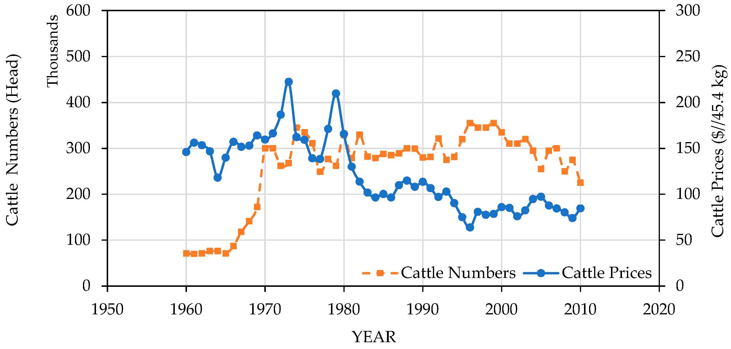
Previous studies (e.g., [19]) indicated that an increase in cattle inventory (i.e., numbers) can lead to an increase in beef supply, which can result in a decline in cattle prices. Our finding provides a confirmation of this observation. The numbers of heifers (excluding replacement) and steers were negatively related with cattle prices (β = −0.000153; p < 0.0001) and explained 80% of their variation (Table 3). As shown in Figure 11, the opposite relationship between cattle prices and the numbers of heifers (excluding replacement) and steers was approximately consistent over the entire period (i.e., 1960–2010).
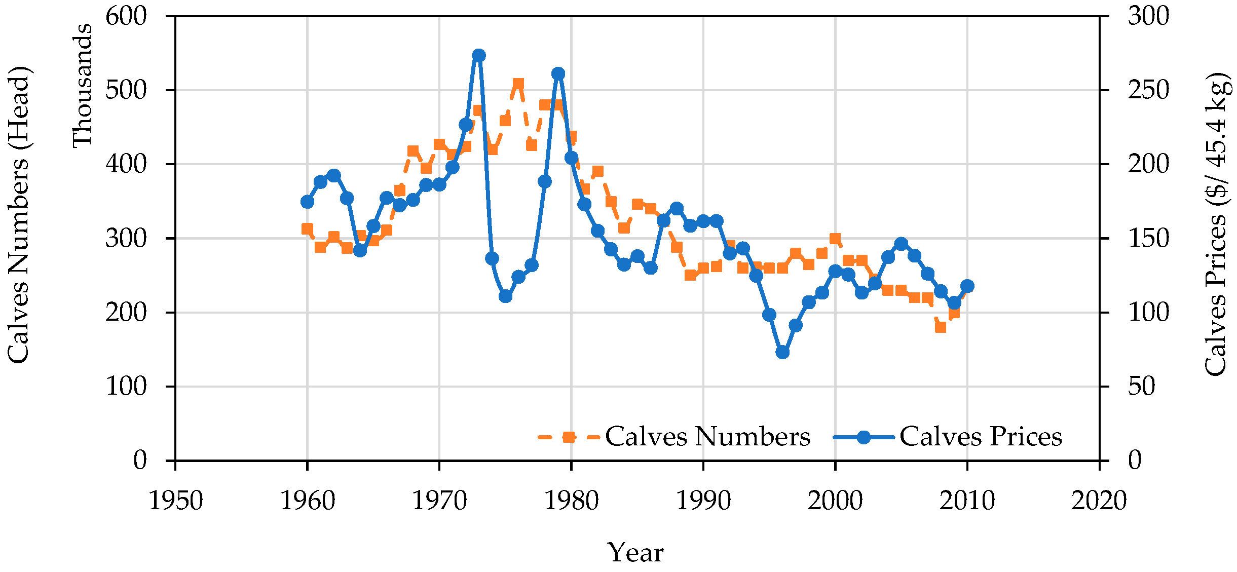
The results also showed how calf prices tend to increase when calf numbers increase (β = 0.000229; p < 0.0001) (Table 3). During the 1964–1974 and 1989–1991 periods, increased calf numbers were concurrent with a rise in prices (Figure 12). However, this finding did not agree with the supply and demand concept that suggest that increased calf numbers can lead to a decline in calf prices [19]. Traditionally, NM’s ranchers tend to sell their animals during the fall months. Moreover, during wet years when rangelands are in good conditions, ranchers tend to postpone selling calves until the spring as short yearlings, or to the following fall as long yearlings, if calf weight is not satisfactory, and predicted prices are satisfying [23]. This traditional marketing practices can result in reduced calf supply during certain years, which can, consequently, result in increased prices.
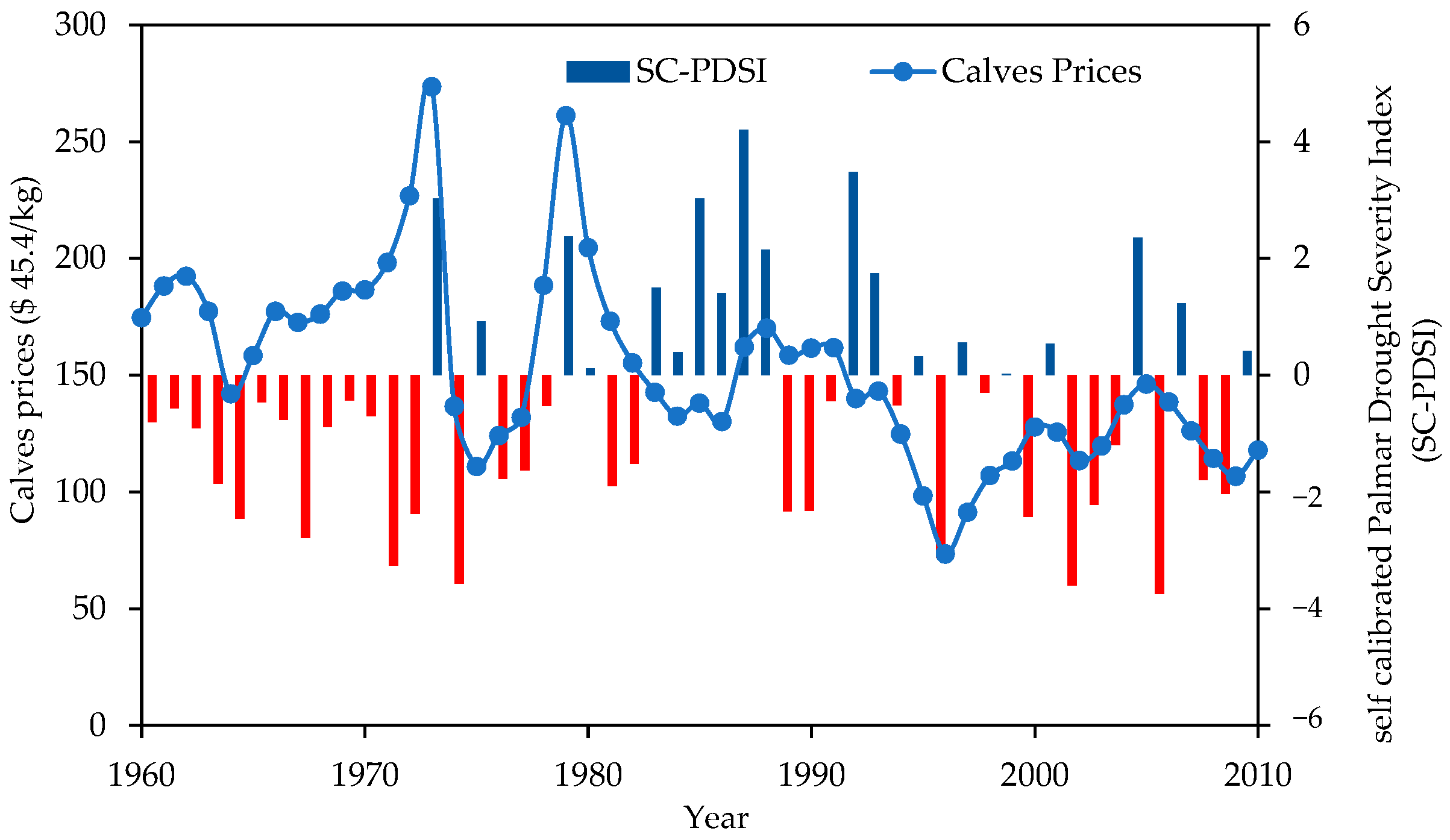
The SC-PDSI was significantly correlated with prices of beef cattle (β = 2.2126; p = 0.0005) and calves (β = 2.5337; p = 0.0014), and it explained about 80% and 60% of their variation, respectively (Table 3). In 1973, it was observed that the SC-PDSI was 3.03-indicating severe wet spell-and cattle and calf prices were $222.4 and $273.5, respectively (Figure 13 and Figure 14). However, the 1974 drought was one of most severe events that affected the USA [2], and during that year, the SC-PDSI was −3.03, indicating severe drought conditions that were associated with a decline in prices of cattle and calves to $162.2 and $136.6, respectively. This decline in prices can be attributed to herd liquidation during drought periods [6,23]. Our findings are in agreements with Countryman et al. [46], who reported that cattle price decreases shortly after drought, while cattle inventory decreases over the long term after droughts.

3.4.2. Evaluation of Production and Drought Relationship

The relationship between drought and cattle numbers by class was further evaluated using regression analysis. The results (not shown) indicated that the number of all cattle classes did not show any significant relationship with drought. This can partly be due to the biological nature of cattle production [10]. For example, when a drought event is over, cow-calf producers react to suitable rangelands forage conditions by holding back more replacement heifers and not culling as many cows, but it is known that heifers that are kept to increase the herd size cannot increase calf numbers for at least three years [10]. However, ranchers’ decisions may not solely be based on income and profit reasons. In some cases, management decisions at a farm level may be based on social, well-being, and traditional cultural aspects due to farmers connectedness to their cultural values and production species [47]. Thus, they may be willing to keep animals even if prices are low and feed is limited.
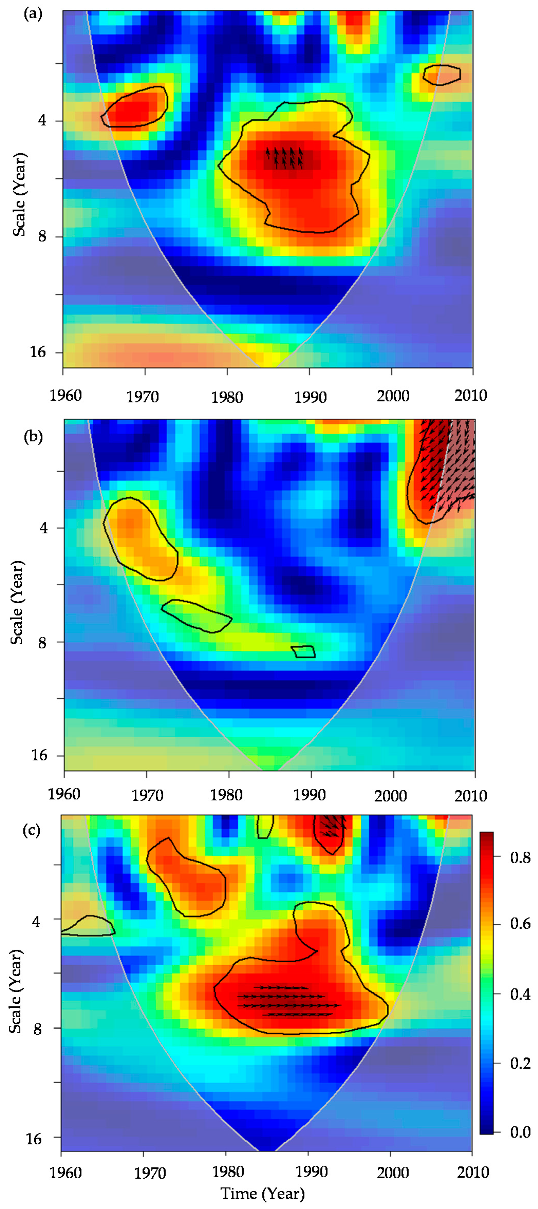
An additional evaluation using coherence analysis was conducted to affirm the finding above and the results are shown in Figure 15. The results indicated that there was no consistent coherence between drought and cattle production cycles throughout the study period but appeared only during some discrete periods. For example, during the 1965–1974 and 2005–2008 periods, the SC-PDSI showed a strong relationship with replacement heifers’ numbers. Both timeseries moved together at scale of four to five years. However, in the 1980–1997 period, there was a lead/lag phase relation between these variables on a scale of four to five years. Wet years can lead to an increase in replacement heifers, but the increase may have required four to five years.
On the other hand, the SC-PDSI showed a strong to moderate relationship with numbers of heifers (excluding replacement) and steers between 1965 and 1981, and the two variables followed the same behavior. In contrast, during the 2005–2010 period, there was a lead/lag phase relationship between these variables, and the lag was estimated by three to four years (Figure 15b).
Moreover, the SC-PDSI had a strong relationship with numbers of calves between 1980 and 1982, and they both moved together on a scale of one to four years. The lag phase relation between these variables was observed during the 1983–1994 and 1994–1996 periods, and the estimated lag was five to six years (Figure 15c).
Some previous studies indicated that NM’s beef cattle population decreases when drought occurs due to herd liquidation, whereas it increases during favorable conditions [4,7,23]. Our coherence analysis results supported the finding that ranchers tend to increase the herd size when favorable conditions occur (especially precipitation and temperature) [4,23], but due to the biological nature beef cattle production, the increase in beef cattle numbers is expected to occur after not less than three years [10].

3.4.3. Multilinear Regressions

Based on the evaluation of the relationships between drought and production described above (Section 3.4.2), a multilinear regression can be assessed between prices, production, and drought with minimal to no effects of multicollinearity between the independent variables (i.e., drought and cattle numbers). This assessment can help in identify what model form (simple linear versus multilinear) can better represent and account for most of the variations in cattle prices. Multilinear regressions between cattle prices and the number of the different cattle classes as well as drought (SC-PDSI) were developed and shown in Table 4. The results showed similar indications to those presented in Table 3, which suggested that the number of replacement heifers was not a significant predictor of cattle prices while both drought (with positive correlations) and number of heifers (excluding replacement) and steers (negative correlations) can affect cattle prices. A one step lag of prices was also considered in the model. The regression model explained 85% of the variation in cattle prices. On the other hand, the multilinear regression between calf prices and calf numbers and drought explained about 64% of the variations in prices. Calf number was a significant predictor (p ≤ 0.0001) while drought (p = 0.4805) was not.

3.5. Drought and Net Return

The effect of drought on ranch net return was evaluated over New Mexico, considering medium and large ranch sizes as well as for the combined data [referred to All] as shown in Table 5. The three multilinear regression models for all, large, and medium ranch sized were able to predict about 51%, 62%, and 43% of the variations in the net return, respectively. It appeared that the ranch net return in New Mexico regardless of the ranch size was significantly (p < 0.0001) correlated with SC-PDSI and showed positive relationships. Using the typical ranges of the PDSI for the identified drought severity categories (Section 2.3) [40], different SC-PDSI values were used in developing a net return-drought model. Our finding indicated that a rancher can still obtain positive net returns when a drought falls with within “Abnormally Dry” category (i.e., D0 or PDSI = −1.0 to −1.9). However, a rancher with a large herd size (200–400 head) can endure drought conditions better than those with a medium herd size and reach the breakeven point. For example, at a SC-PDSI of −3.38 (i.e., within the D2 drought category or “Severe Drought”) the net return is zero for large herd sizes while medium herd sizes can be at a breakeven point (zero net return) at a SC-PDSI of −2.9 (i.e., within the D1 drought category or “Moderate Drought”). In other words, the net return of a ranch ($/head) is expected to increase (or decrease) by $62.29, $60.51, and $64.07 per head if the SC-PDSI increase (or decrease) by one unit in all, large, and medium ranch sizes, respectively.

3.6. Implications, Limitations, and Future Directions

The evaluated ranch net return used in this study was based on limited survey datasets that was available for only 10 years (2010–2019) compared to those for price and production data (1960–2010). Thus, the developed net return and price models should not be considered as conclusive and, therefore, needs further improvement by including longer timeseries of ranch budget data. Moreover, the developed ranch net return–drought models in this analysis considered only two commonly identified ranch sizes (i.e., medium and large) as the data for other ranch sizes (i.e., small and extra-large) are not commonly available in New Mexico. However, for proper representation of ranch return for New Mexico, all ranch sizes should be included in the future to appropriately upscale the survey data to the state level. Another limitation of the ranch data was related to the fact that the data did not overlap with the prices and production data. This mismatch in the data periods did not capture a common period during which extreme environmental events and socioeconomic fluctuations had occurred. Moreover, as indicated in the USDA-NASS reports, the reporting of cattle and calf prices was discontinued since 2010. This data discontinuity poses additional challenges to conduct similar analysis in the future and update these findings. This highlights the need to continue collective survey data such as those conducted by NMSU.
Moreover, other factors may play a role in identifying ranch net returns as indicated by NMSU [34]. Regardless of these limitations, the estimated variations in the ranch net return due to drought should provide reasonable indications of the potential impacts of future drought conditions on ranch management. The findings of this study can be used as a general indication to when a rancher should sell calves, what should be a suitable timing of breeding to maximise the economic return, as well as other ranch management decisions. One of the anticipated future directions for this study is the development of a user-friendly and ready-to-use software (e.g., accessed in hand-held devices) that can be shared with ranchers and other stakeholders to help in the decision-making process.
While this study was conducted using data for New Mexico, the state can be considered as a prototype that represents dryland conditions and regional market fluctuation. Thus, the findings can regionally be expanded over the southwestern US including the states of Arizona, Nevada, California, as well as regions in other parts of the world with similar environmental characteristics. However, it is recommended that similar analyses be conducted in other states of this region to validate these findings.

4. Conclusions

This analysis was conducted within the context of developing an integrated model of food-energy-water systems for New Mexico, USA. The study evaluated monthly and annual price patterns and cycles of cattle and calves; the relationships between annual cattle prices and numbers and drought; and the effects of drought on ranch net return in New Mexico for the 1960–2010 and 2010–2019 periods. New Mexico’s cattle and calf prices showed a decreasing trend since 1980. Seasonally, cattle monthly prices tended to decrease in January to December and increase in February to May, while those for calves behaved slightly differently as they increased in February to July. The highest prices for both were observed in April. It was noticed that cattle and calf prices decreased with improved drought conditions. On the other hand, cattle prices decreased with increased numbers of replacement heifers and steers, while calf prices increased with increased calf numbers. Annual cattle and calf prices showed six- and 10-year cycles, while their inventory showed six- and eight- year cycles, respectively. Improved drought conditions can result in increased ranch net return. Our findings suggested that a rancher can still obtain positive net return if there is a drought that falls within the D0 “Abnormally Dry” category. However, a rancher with a large herd size (200–400 head) can endure drought better than a rancher with medium herd size, as medium sized ranches reach the breakeven point more quickly. Specifically, it appeared that the net return ($/head) is expected to increase (or decrease) by $62.29, $60.51, and $64.07 per head if the SC-PDSI increase (or decrease) by one unit in all, large, and medium ranch sizes, respectively. These estimated net returns based on drought need further refinement using additional data. The findings of this study can provide very important description and characterization of price fluctuations of beef cattle and can help in identifying the factors that affect these production systems in New Mexico. This information, if applied, can help ranchers and decision makers in New Mexico and in other similar regions to make informed ranch management decisions in response to drought. For example, these finding can help ranchers make decisions about when to increase or decrease the herd size during favorable or drought conditions (i.e., when to sell calves and at what weight or age, and timing of breeding). In addition, we emphasize that ranchers should consider the risk of using such predictions since natural and social systems do not always follow consistent patterns. Moreover, these findings can support the development of improved understanding of beef cattle production systems in New Mexico, southwestern US, and other regions with similar characteristics.

Author Contributions

Conceptualization, A.J.Z. and H.M.E.G.; methodology, A.J.Z., H.M.E.G., J.L.H., S.A.I., M.N.S. and A.F.C.; software, A.J.Z., M.N.S., S.A.I., M.G.G. and C.C.G.; validation, A.J.Z., H.M.E.G., J.L.H., A.F.C. and M.N.S.; formal analysis, A.J.Z. and C.C.G.; investigation, A.J.Z. and H.M.E.G.; resources, H.M.E.G.; data curation, A.J.Z.; writing—original draft, A.J.Z.; writing—review and editing, A.J.Z., H.M.E.G., J.L.H., M.N.S., A.F.C., C.C.G. and G.L.T.; visualization, A.J.Z., M.N.S. and H.M.E.G.; supervision, H.M.E.G. and A.F.C.; project administration, H.M.E.G.; funding acquisition, H.M.E.G. and A.J.Z. All authors have read and agreed to the published version of the manuscript.

Funding

This research was partially funded by the National Science Foundation (NSF), awards # 1739835 and # IIA-1301346, New Mexico State University, and Canadian Bureau of International Education (CBIE) -Libyan-North American Scholarship Program (LNASP).

Institutional Review Board Statement

Not applicable.

Informed Consent Statement

Not applicable.

Data Availability Statement

All data used in this study are publicly available and references with access links are cited in where appropriate in this article.

Acknowledgments

The authors would like to thank three anonymous reviewers for their effort and comments that helped in strengthening the manuscript.

Conflicts of Interest

The authors declare no conflict of interest. The funders had no role in the design of the study; in the collection, analyses, or interpretation of data; in the writing of the manuscript, or in the decision to publish the results. Any opinions, findings, and conclusions or recommendations expressed in this material are those of the author(s) and do not necessarily reflect the views of the National Science Foundation.

References

  1. Yadav, K.; Geli, H.; Cibils, A.F.; Hayes, M.; Fernald, A.; Peach, J.; Sawalhah, M.N.; Tidwell, V.C.; Johnson, L.E.; Zaied, A.J.; et al. An Integrated Food, Energy, and Water Nexus, Human Wellbeing, and Resilience (FEW-WISE) Framework: New Mexico. Front. Environ. Sci. 2021, 9, 667018. [Google Scholar] [CrossRef]
  2. Sawalhah, M.N.; Holechek, J.L.; Cibils, A.F.; Geli, H.M.E.; Zaied, A. Rangeland Livestock Production in Relation to Climate and Vegetation Trends in New Mexico. Rangel. Ecol. Manag. 2019, 72, 832–845. [Google Scholar] [CrossRef]
  3. Holechek, J.L.; Geli, H.M.; Cibils, A.F.; Sawalhah, M.N. Climate Change, Rangelands, and Sustainability of Ranching in the Western United States. Sustainability 2020, 12, 4942. [Google Scholar] [CrossRef]
  4. Zaied, A.J.; Geli, H.M.E.; Holechek, J.L.; Cibils, A.F.; Sawalhah, M.N.; Gard, C.C. An Evaluation of Historical Trends in New Mexico Beef Cattle Production in Relation to Climate and Energy. Sustainability 2019, 11, 6840. [Google Scholar] [CrossRef] [Green Version]
  5. Johnson, L.E.; Geli, H.M.E.; Hayes, M.J.; Smith, K.H. Building an Improved Drought Climatology Using Updated Drought Tools: A New Mexico Food-Energy-Water (FEW) Systems Focus. Front. Clim. 2020, 2. [Google Scholar] [CrossRef]
  6. Holechek, J.L. Drought and Low Cattle Prices: Hardship for New Mexico Ranchers. Rangelands 1996, 18, 11–13. [Google Scholar]
  7. Holechek, J.L. Drought in New Mexico: Prospects and Management. Rangelands 1996, 18, 225–227. [Google Scholar]
  8. WRI Aqueduct Water Risk Atlas—World Resources Institute. Available online: https://www.wri.org/resources/maps/aqueduct-water-risk-atlas (accessed on 4 January 2020).
  9. Searchinger, T.; Waite, R.; Hanson, C.; Ranganathan, J.; Dumas, P.; Matthews, E.; Klirs, C. Creating a Sustainable Food Future: A Menu of Solutions to Feed Nearly 10 Billion People by 2050. Final Report; World Research Institute: Washington, DC, USA, 2019; pp. 1–556. [Google Scholar]
  10. Anderson, D.P.; Robb, J.G.; Mintert, J. The Cattle Cycle. Managing for Today’s Cattle Market and beyond. 1996. Available online: http://valueaddedag.org/TodaysCattlePub.html (accessed on 12 September 2021).
  11. Herring, A.D. Beef Cattle Production Systems; CABI: Oxfordshire, UK, 2014. [Google Scholar]
  12. Schroeder, T.; Marsh, T.; Mintert, J. Beef Demand Determinants. Report Prepared for the Joint Evaluation Advisory Committee; Department of Agricultural Economics, Kansas State University: Manhattan, KS, USA, 2000; 61p. [Google Scholar]
  13. Maia de Souza, D.; Petre, R.; Jackson, F.; Hadarits, M.; Pogue, S.; Carlyle, C.N.; Bork, E.; McAllister, T. A Review of Sustainability Enhancements in the Beef Value Chain: State-of-the-Art and Recommendations for Future Improvements. Animals 2017, 7, 26. [Google Scholar] [CrossRef]
  14. Tonsor, G.T.; Olynk, N.J. Impacts of Animal Well-being and Welfare Media on Meat Demand. J. Agric. Econ. 2011, 62, 59–72. [Google Scholar] [CrossRef]
  15. Chavas, J.-P. On Information and Market Dynamics: The Case of the US Beef Market. J. Econ. Dyn. Control 2000, 24, 833–853. [Google Scholar] [CrossRef]
  16. Culbert, J.I. Cattle Industry of New Mexico. Econ. Geogr. 1941, 17, 155–168. [Google Scholar] [CrossRef]
  17. USDA—National Agricultural Statistics Service—New Mexico. Quick Stats (Searchable Database) and Annual Statistical Bulletin. Available online: https://www.nass.usda.gov/Statistics_by_State/New_Mexico/index.php (accessed on 28 March 2019).
  18. Brooks, K. Annual and Seasonal Price Patterns for Cattle; University of Nebraska-Lincoln, Department of Agricultural Economics: Lincoln, NE, USA, 2015. [Google Scholar] [CrossRef]
  19. Prevatt, J.W.; VanSickle, J.J. United States Cattle Cycles: Perspectives on US Cattle and Calves Inventories and Prices; Food and Resource Economics Department, Institute of Food and Agricultural: Gainesville, FL, USA, 2000. [Google Scholar]
  20. Holechek, J.L.; Pieper, R.D.; Herbel, C.H. Range Management: Principles and Practices, 6th ed.; Prentice-Hall: Hoboken, NJ, USA, 1989. [Google Scholar]
  21. Jarvis, L.S. Cattle as Capital Goods and Ranchers as Portfolio Managers: An Application to the Argentine Cattle Sector. J. Polit. Econ. 1974, 82, 489–520. [Google Scholar] [CrossRef]
  22. Rosen, S. Dynamic Animal Economics. Am. J. Agric. Econ. 1987, 69, 547–557. [Google Scholar] [CrossRef]
  23. Boykin, C.C.; Gray, J.R.; Caton, D.D. Ranch Production Adjustments to Drought in Eastern New Mexico; Agricultural Experiment Station, New Mexico State University, in Cooperation with Farm Economics Division, Economic Records Service, United States Department of Agriculture: Las Cruces, NM, USA, 1962. [Google Scholar]
  24. Sawalhah, M.N.; Geli, H.M.E.; Holechek, J.L.; Cibils, A.F.; Spiegal, S.; Gifford, C. Water Footprint of Rangeland Beef Production in the Southwestern United States. Water 2021, 13, 1950. [Google Scholar] [CrossRef]
  25. Foran, B.D.; Smith, D.S. Risk, Biology and Drought Management Strategies for Cattle Stations in Central Australia. J. Environ. Manag. 1991, 33, 17–33. [Google Scholar] [CrossRef]
  26. Hall, D.C.; Knight, T.O.; Coble, K.H.; Baquet, A.E.; Patrick, G.F. Analysis of Beef Producers’ Risk Management Perceptions and Desire for Further Risk Management Education. Rev. Agric. Econ. 2003, 25, 430–448. [Google Scholar] [CrossRef]
  27. Herbel, C.H.; Ares, F.N.; Wright, R.A. Drought Effects on a Semidesert Grassland Range. Ecology 1972, 53, 1084–1093. [Google Scholar] [CrossRef]
  28. Pieper, R.D.; Parker, E.E.; Donart, G.B.; Wright, J.D. Cattle and Vegetation Response to Four-Pasture and Continuous Grazing Systems. Agric. Exp. Stn. Bull. 1991, 756. [Google Scholar]
  29. Gedefaw, M.G.; Geli, H.M.E.; Abera, T.A. Assessment of Rangeland Degradation in New Mexico Using Time Series Segmentation and Residual Trend Analysis (TSS-RESTREND). Remote Sens. 2021, 13, 1618. [Google Scholar] [CrossRef]
  30. Regional Climate Centers. Climate of New Mexico. Available online: https://www.ncdc.noaa.gov/customer-support/partnerships/regional-climate-centers (accessed on 28 July 2019).
  31. Stoddart, L.A.; Smith, A.D.; Thadis, W. Range Management, 3rd ed.; McGraw Hill: New York, NY, USA, 1975. [Google Scholar]
  32. Desert Research Institute, Western Regional Climate Center. Available online: https://wrcc.dri.edu/ (accessed on 6 June 2020).
  33. Federal Reserve Economic Data|FRED|St. Louis Fed. Available online: https://fred.stlouisfed.org/ (accessed on 28 March 2019).
  34. NMSU: Cost and Return Estimates for Farms and Ranches—CARE. Available online: https://aces.nmsu.edu/cropcosts/index.html (accessed on 8 June 2021).
  35. López, S.; Cibils, A.; Smedly, U.; Guldan, S.; Fernald, A.; Ochoa, C.; Boykin, K.; Cibils, L. Linkages Between Acequia Farming and Rangeland Grazing in Traditional Agropastoral Communities of the Southwestern USA. Sustainability 2018, 10, 2021. [Google Scholar] [CrossRef] [Green Version]
  36. SAS Help Center: PROC AUTOREG Statement. Available online: https://documentation.sas.com/?cdcId=pgmsascdc&cdcVersion=9.4_3.4&docsetId=etsug&docsetTarget=etsug_autoreg_syntax02.htm&locale=en#etsug_autoreg004406 (accessed on 17 March 2021).
  37. Spectral Plots. Available online: www.ibm.com/support/knowledgecenter/sslvmb_sub/statistics_mainhelp_ddita/spss/trends/idh_spec.html (accessed on 17 March 2021).
  38. EViews Help: Seasonal Adjustment. Available online: http://www.eviews.com/help/helpintro.html#page/content/series-Seasonal_Adjustment.html (accessed on 17 March 2021).
  39. R: The R Project for Statistical Computing. Available online: https://www.r-project.org/ (accessed on 17 March 2021).
  40. Drought Classification|U.S. Drought Monitor. Available online: https://droughtmonitor.unl.edu/About/AbouttheData/DroughtClassification.aspx (accessed on 8 June 2021).
  41. Tester, C.A.; Popp, M.P.; Kemper, N.P.; Nalley, L.L.; West, G. Impact of Weather and Herd Size Management on Beef Cow Profitability. J. Agric. Appl. Econ. 2019, 51, 545–567. [Google Scholar] [CrossRef] [Green Version]
  42. Schulz, L. Has the Cattle Cycle Peaked? 2019. Available online: https://lib.dr.iastate.edu/econ_las_pubs/721 (accessed on 13 September 2021).
  43. Fliessbach, A.; Ihle, R. Cycles in Cattle and Hog Prices in South America. Aust. J. Agric. Resour. Econ. 2020, 64, 1167–1183. [Google Scholar] [CrossRef]
  44. Martinez, C.C.; Maples, J.G.; Benavidez, J. Beef Cattle Markets and Covid-19. Appl. Econ. Perspect. Policy 2021, 43, 304–314. [Google Scholar] [CrossRef]
  45. Patalee, B.; Tonsor, G.T. Weather Effects on US Cow-calf Production: A Long-term Panel Analysis. Agribusiness 2021. [Google Scholar] [CrossRef]
  46. Countryman, A.M.; Paarlberg, P.L.; Lee, J.G. Dynamic Effects of Drought on the US Beef Supply Chain. Agric. Resour. Econ. Rev. 2016, 45, 459–484. [Google Scholar] [CrossRef] [Green Version]
  47. Torell, L.A.; Rimbey, N.R.; Ramirez, O.A.; McCollum, D.W. Income Earning Potential versus Consumptive Amenities in Determining Ranchland Values. J. Agric. Resour. Econ. 2005, 30, 537–560. [Google Scholar]
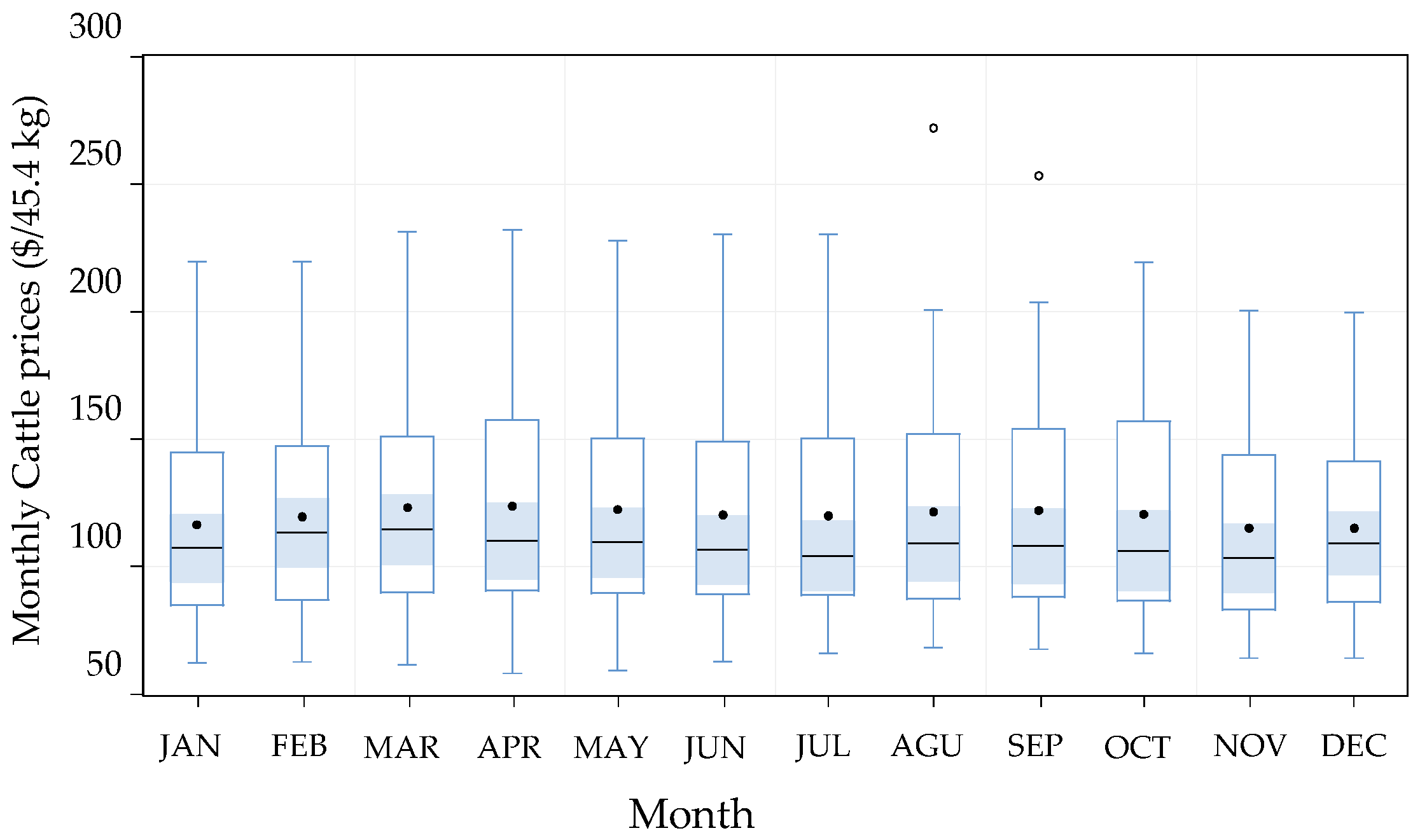
Figure 1. Monthly price patterns for heifers and steers ($/45.4 kg) in New Mexico between 1960 and 2010. The graph shows the values of cattle prices’ mean (back dots within the boxes), median (solid horizontal line within the boxes), the upper and lower limits (upper and lower edges of the boxes), and the 95% confidence intervals for the median (vertical lines outside the boxes). The hollow dots outside the boxes represent outliers in the data.
Sustainability 13 10420 g001
Figure 2. Monthly price patterns for calf ($/45.4 kg) in New Mexico between 1960 and 2010. The graph shows the values of calf prices’ mean (back dots within the boxes), median (solid horizontal line within the boxes), the upper and lower limits (upper and lower edges of the boxes), and the 95% confidence intervals for the median (vertical lines outside the boxes). The hollow dots outside the boxes represent outliers in the data.
Sustainability 13 10420 g002
Figure 3. The periodograms of cattle and calf prices timeseries developed using spectral analysis. The x-axis showed the period in years in logarithmic scale (e.g., 10 refer to 10 years). The y-axis showed the periodogram values (unitless). An identified periodogram peak value would indicate the dominance of a corresponding frequency (period) in the timeseries of the variable of interest. The identified length of cattle and calf prices cycles in New Mexico between 1960 and 2010 were about six and 10 years, respectively.
Sustainability 13 10420 g003
Figure 4. The timeseries components that include actual prices ($/45.4 kg) (top panel), trend (middle panel), and smoothed seasonality (bottom panel) for heifers and steers (that are more than one year old and weigh more than 226.7 kg) prices in New Mexico between 1960 and 2010. The figure indicated a six-year cycle. Each cycle is represented by a peak value, for example in year 1965 for the first identified cycle, which started in 1960 and ended in 1966.
Sustainability 13 10420 g004
Figure 5. The timeseries components that include actual prices ($/45.4 kg) (top panel), trend (middle panel), and smoothed seasonality (bottom panel) for calf prices in New Mexico between 1960 and 2010. The figure indicated a 10-year cycle. Each cycle is represented by a peak value, for example in year 1970 for the first identified cycle that started in 1965 and ended in 1975.
Sustainability 13 10420 g005
Figure 6. The periodograms of cattle (heifers exclude replacement and steers) (left) and calf numbers (right) timeseries developed using spectral analysis. The x-axis showed the period in years in logarithmic scale (e.g., 10 refer to 10 years). The y-axis showed the periodogram values (unitless). An identified periodogram peak value would indicate the dominance of a corresponding frequency (period) in the timeseries of the variable of interest. The identified length of cattle numbers (heifers exclude replacement and steers) (left) and calf number (right) cycles in New Mexico between 1960 and 2010 were about six and eight years, respectively.
Sustainability 13 10420 g006
Figure 7. The timeseries components including the actual numbers (top panel), trend (middle panel), and smoothed seasonality (bottom panel) for cattle (heifers exclude replacement and steers) numbers in New Mexico between 1960 and 2010. The figure indicated a six-year cycle. Each cycle is represented by a peak value, for example in year 1964 for the first identified cycle, which started in 1962 and ended in 1968.
Sustainability 13 10420 g007
Figure 8. The timeseries components that include the numbers (top panel), trend (middle panel), and smoothed seasonality (bottom panel) for calf numbers in New Mexico between 1960 and 2010. The figure indicated an eight-year cycle. Each cycle is represented by a peak value, for example in year 1964 for the first identified cycle, which started in 1962 and ended in 1968.
Sustainability 13 10420 g008
Figure 9. The periodogram of Self-calibrated Palmer Severity Drought Index (SC-PDSI) timeseries developed using spectral analysis. The x-axis showed the period in years in logarithmic scale (e.g., 10 refer to 10 years). The y-axis showed the periodogram values (unitless). An identified periodogram peak value would indicate the dominance of a corresponding frequency (period) in the timeseries of the variable of interest. The identified length the SC-PDSI cycle in New Mexico between 1960 and 2010 was about six years.
Sustainability 13 10420 g009
Figure 10. The timeseries components that include the values (unitless) (top panel), trend (middle panel), and smoothed seasonality (bottom panel) for the Self-calibrated Palmer Severity Drought Index (SC-PDSI) in New Mexico between 1960 and 2010. The figure indicated a six-year cycle. Each cycle is represented by a peak value, for example in year 1963 for the first identified cycle, which started in 1960 and ended in 1966.
Sustainability 13 10420 g010
Figure 11. The numbers of heifers (excluding replacement) and steers (more than one year old and weight more than 226.7 kg) with cattle prices ($/45.4 kg) in New Mexico for the 1960–2010 period.
Sustainability 13 10420 g011
Figure 12. Calf numbers and prices ($/45.4 kg) in New Mexico for the 1960–2010 period.
Sustainability 13 10420 g012
Figure 13. The Self-calibrated Palmer Severity Drought Index (SC-PDSI) and cattle prices ($/45.4 kg) in New Mexico for the 1960–2010 period. The blue bars of the SC-PDSI indicate positive values or wet conditions (i.e., no drought), while the red bars indicate negative values representing different levels of drought severity as identified by the USDM [40]. For example, values of SC-PDSI between −2 and −2.9 indicate Moderate Drought conditions.
Sustainability 13 10420 g013
Figure 14. The Self-calibrated Palmer Severity Drought Index (SC-PDSI) and calf prices ($/45.4 kg) in New Mexico for the 1960–2010 period. The blue bars of the SC-PDSI indicate positive values or wet conditions (i.e., no drought), while the red bars indicate negative values representing different levels of drought severity as identified by the USDM [40]. For example, values of SC-PDSI between −2 and −2.9 indicate Moderate Drought conditions.
Sustainability 13 10420 g014
Figure 15. Bivariate wavelet coherency between (a) SC-PDSI and replacement heifers’ numbers, (b) SC-PDSI and numbers of heifers (exclude replacement) and steers, and (c) SC-PDSI and calf numbers in New Mexico between 1960 and 2010. The value of the coherences (ranging from 0 to 1 unitless) between two variables was represented by the scale bar with blue and red indicating low to high coherence, respectively. Arrows represent the lead/lag phase relationship between the examined series. Solid lines show the cones of influence. Thin line and shaded cone area represent error in timeseries. Thick solid lines show the 95% confidence levels. Arrows pointing to the left-up and right-down indicate that the first variable (SC-PDSI) is leading. Arrows pointing to the left-down show that the second variable is leading. Arrows pointing to the right show that the two-time series move in the same direction. Zero-phase difference indicates that the two-time series move in together on a particular scale.
Sustainability 13 10420 g015
Table 1. Monthly price ($/45.4 kg) pattern and variability by cattle class in New Mexico between 1960 and 2010.
JanuaryFebruaryMarchAprilMayJuneJulyAugustSeptemberOctoberNovemberDecember
Heifers and steers
Price pattern116.5119.7123.2123.8122.4120.3120121.6122.1121.6115.3115.1
Std Dev37.437.93939.239.238.339.541.740.441.736.837
Calf
Price pattern145.5153.6156157.5154.5150.9150.6153.1151.3149.4149149.2
Std Dev43.14040.938.940.438.738.744.142.342.341.539.7
Heifers and steers represent all those that are more than one year old and weigh more than 226.7 kg. Calf represents all those that are less than one year old and weigh less than 226.7 kg.
Table 2. Mean annual prices ($/45.4 kg) and percentage of change by cattle class in New Mexico during the five decades from 1960 to 2010.
Year
Count
1960–19701970–19801980–19901990–20002000–2010
$/45.4 kg% Change$/45.4 kg% Change$/45.4 kg% Change$/45.4 kg% Change$/45.4 kg% Change
Cattle Prices
1145.9 159.5 165.6 113.4 85.8
2156.16.9166.44.3129.9−21.5106.6−685.2−0.7
3153.5−1.6186.612.1113.6−12.596.9−976−10.8
4146.6−4.4222.419.1101.8−10.4102.7682.388.3
5118.1−19.4162.2−27.096.5−5.190.3−12.194.614.9
6139.718.3159.2−1.8100.13.774.9−16.997.12.6
7157.212.4139.09−12.696.4−3.663.8−14.887.7−9.6
8151.6−3.5138.5−0.4109.713.780.826.684.5−3.6
9152.90.86171.123.5114.84.677.5−480.3−5
101647.2209.722.5108−5.978.51.274.09−7.7
Calf Prices
1174.7 186.4 204.5 161.5 125.6
2188.27.7198.16.2173.1−15.3161.70.09113.4−9.6
3192.42.2226.814.4155.2−10.3140−13.4119.75.5
4177.2−7.8273.520.5142.7−8143.22.3137.3714.7
5142−19.8136.6−50132.4−7.2124.89−12.8146.26.4
6158.4811.5111−18.71384.298.4−21.1138.4−5.3
7177.311.9124.111.8130.1−5.773.4−25.4126.2−8.8
8172.57−2.61326.3162.124.691.424.5114.4−9.3
9176.12188.542.7170.14.910717106.7−6.7
101865.6261.0938.4158.6−6.7113.35.911810.5
Year count is the year within each decade with year 10 being the one before the beginning of a new decade (e.g., year 10 in the 1960–1970 decade is 1969). The % change was estimated with respect to the previous year.
Table 3. Independent variables related with historical trends in cattle prices by class in New Mexico. Each predictor was modeled individually of the others using an exponential generalized autoregressive conditional heteroscedasticity model (EGARCH).
Dependent VariableIndependent Variable ModelInterceptEstimate (β)AR1p-ValueR2
Cattle Prices ($/45.4 kg)Number of Replacement Heifers EGARCH142.4881−8.737 × 10⁻⁶ 0.9684
Number of Heifers (Excluding Replacement) and SteersEGARCH149.5517−0.000153−0.950<0.00010.8
SC-PDSIEGARCH148.60332.2126−0.9730.00050.8
Calf Prices ($/45.4 kg)Number of CalvesEGARCH82.85920.000229−1.0308<0.00010.6
SC-PDSIEGARCH158.8782.5337−1.20270.00140.6
Table 4. Independent variables related with historical trends in cattle prices by class in State of New Mexico. Multilinear regressions between prices and numbers and drought were modeled using an exponential generalized autoregressive conditional heteroscedasticity model (EGARCH).
Dependent VariableVariablesEstimate p-ValueR2
Cattle Prices ($/45.4 kg)Intercept154.26980.0004
Number of Replacement Heifers −0.0000180.9
Number of Heifers (Excluding Replacement) and Steers−0.0001090.040.85
SC-PDSI1.85060.0004
AR1−0.9784<0.0001
Calf Prices ($/45.4 kg)Intercept83.4322<0.0001
Number of Calves0.000227<0.00010.64
SC-PDSI0.66870.4805
AR1−1.0711<0.0001
AR20.3739<0.0001
Table 5. Independent variable that includes SC-PDSI evaluated against net return in New Mexico using multilinear regressions using survey data for ranch budgets for the period between 2010 and 2019 over large, medium, and both ranch sizes.
Ranch SizeDependent VariableVariable Estimatep-ValueR2
AllNet Return ($/head)Intercept195.65<0.00010.51
SC-PDSI62.29<0.0001
LargeNet Return ($/head)Intercept204.66<0.00010.62
SC-PDSI60.51<0.0001
Intercept186.64<0.00010.43
MediumNet Return ($/head)SC-PDSI64.07<0.0001
Publisher’s Note: MDPI stays neutral with regard to jurisdictional claims in published maps and institutional affiliations.