Traffic Volume Prediction: A Fusion Deep Learning Model Considering Spatial–Temporal Correlation

Abstract

In this paper, a fusion deep learning model considering spatial–temporal correlation is proposed to solve the problem of urban road traffic flow prediction. Firstly, this paper holds that the traffic flow of a section in the urban road network not only depends on the fluctuation of its own time series, but is also related to the traffic flow of other sections in the whole region. Therefore, a traffic flow similarity measurement method based on wavelet decomposition and dynamic time warping is proposed to screen the sections which are similar to the traffic flow state of the target section. Secondly, in order to improve the prediction accuracy, the unstable time series are reconstructed into stationary time series by differential method. Finally, taking the extracted traffic flow data of a similar section as an independent variable and the traffic flow data of target section as dependent variable, we input the above variables into the proposed CNN-LSTM fusion deep learning model for traffic flow prediction. The results show that the proposed model has a higher accuracy and stability than the other benchmark models. The MAPE can reach 92.68%, 93.39%, 85.14%, and 76.14% at a time interval of 5 min, 15 min, 30 min, and 60 min, and the other evaluation indexes are also better than the rest of the benchmark models.

1. Introduction

With the rapid development of economy and urbanization, the development of urban transportation has made great progress. The high quality and efficient operation of an urban transportation system is not only an important foundation for the development and construction of modern city, but is the main link to maintaining the daily work and life of the city and its surrounding areas. Traffic flow prediction can be defined as the process of estimating the traffic flow state at a future time [1]. Real-time and accurate traffic flow prediction can improve the operation efficiency of urban roads and provide theoretical support for traffic management decision-making. Similarly, accurate predictive information can optimize individual travelers’ travel planning and save on their travel time. Therefore, an accurate traffic flow prediction is a key issue in the development of intelligent transportation systems (ITS) in the future.

Over the past few decades, many different traffic flow prediction approaches have emerged, including parametric models [2], nonparametric models [3,4], artificial intelligence models [5,6], and fusion models [7,8]. Although many advanced methods have emerged to predict the traffic flow in a road section, the following three limitations remain:

(1) Difficulty for researchers to collect high-quality data to describe the road section traffic state at different time intervals;

(2) The traffic characteristics of target sections are affected by other sections in adjacent or regional areas, which requires efficient methods to extract effective information.

(3) Few models can comprehensively consider the spatial–temporal factors affecting the traffic flow of the section and accurately predict it.

To overcome problem (1) and predict the traffic flow efficiently, traffic volume was chosen to represent the road traffic flow state. Compared with other traffic parameters such as occupancy and travel speed, traffic flow can be measured by loop detectors, global positioning systems devices installed on floating cars and remote traffic microwave sensors (RTMS) mounted on the side of the road. As the most popular non-intrusive traffic detectors, the remote traffic microwave sensor does not cause temporary lane closures for its installation or traffic flow interruption. Moreover, they can detect traffic volume, occupancy, and speed in multiple lanes without causing interference [9]. In addition, the research conducted by Yu and Prevedouros revealed that the volume measurement of RTMS can achieve up to 95% accuracy in heavy but non-congested traffic, higher than the measurement accuracy of traffic speed (91%) and other traffic flow parameters, and is higher than that of the autoscope vehicle detection and other sensors [10]. Consequently, we utilized the traffic volume data of lanes captured by RTMS as the predictor in this study.

In recent years, the deep learning model has been widely used in all kinds of big data processing, such as image recognition, language, and digital text. Therefore, combined with the above problems (2) and (3) and deep learning technology, this paper proposes a fusion deep learning model considering spatial–temporal correlation to achieve the accurate prediction of urban road traffic flow. Based on the aforementioned discussion, the improvement and contributions of this study mainly involve the following three aspects:

(1) A road section similarity measurement method based on dynamic time warping and wavelet decomposition is proposed to determine the candidate road section which is similar to the traffic flow state of the target road section.

(2) In order to capture the spatial–temporal features of the travel volume of road sections, a two-layer deep learning structure is proposed, which combines the CNN and the LSTM.

(3) Taking the traffic flow data collected by RTMS detector in Daxing District of Beijing as an example, this paper verifies the accuracy and practicability of the proposed model.

The rest of the paper is arranged as follows: Section 2 summarizes and analyzes the advantages and disadvantages of the existing traffic flow prediction methods. In Section 3, the fusion deep learning model considering spatial–temporal correlation is analyzed in detail. In Section 4, we substitute a specific example into the proposed model and verify the accuracy and practicability of the model by comparing it with others. Section 5 is the conclusion and the future work of this study.

2. Related Work

With the transformation of information collection modes, the presentation format and magnitude of data have changed greatly, such as the data of RTMS, from which derives a variety of methods used to solve the problem of traffic flow prediction.

Traditional traffic prediction methods mainly include the historical average model [11], k-nearest neighbor model [12], and related improved models [13,14,15]. However, due to the traffic flow, the data have the characteristics of high noise and high uncertainty, even if it has obvious periodicity, and makes it difficult for the traditional time series prediction methods to model accurately. In recent years, the machine learning method has been widely used in traffic flow prediction because it can highly adapt to high-noise data, reduce errors by cyclic iteration, and deeply excavate the inherent laws of data. The prediction methods of machine learning mainly include the artificial neural network (ANN) [16], support vector regression (SVR) [17], and so on. However, ANN has a serious overfitting problem, and lacks generalization ability, therefore it is easy to fall into a local optimal problem, and its prediction effect is unsatisfactory. Compared with ANN, SVR has a stronger generalization ability and is not easy to fall into a local optimization problem. For this paper, when a large number of relevant sections are selected, i.e., when the dimension of characteristic variables is high, the operation efficiency of SVR is very slow and dimension reduction needs to be carried out first. However, all dimension reduction methods have the defects of strong subjectivity and low applicability, therefore some features of data may be lost.

Deep learning models can well optimize the above problems and are able to extract deep features from data. Most of the existing studies have predicted time series data by constructing a single deep learning model. For example, Zhang et al. put forward a new deep learning framework to capture the time and spatial correlation of non-stationary time series in a multi-step traffic situation prediction. The results showed that the model has the best prediction effect under various error evaluation parameters [18]. Tian et al. proposed a novel approach based on LSTM to get an accurate result for traffic flow prediction [19]. However, there are always some specific defects in a single deep learning model, which affects the final prediction ability of the model. Therefore, in order to make up for the shortcomings of each model, some studies have used the fusion deep learning model to predict the time series data. For example, Sun et al. put forward a hybrid Kalman filter model to forecast the traffic flow parameters and judge the congestion of the target section according to the forecasted vehicle density [20]. Dong et al. combined a Kalman filter with the autoregressive integrated moving average (ARIMA) model to forecast the traffic flow state of a road section [21]. Narmadha et al. proposed hybrid neural network algorithms such as the convolutional neural network (CNN) and the long short-term memory (LSTM) network for short-term traffic flow prediction based on multivariate analysis [22]. Loan et al. proposed a deep learning based traffic flow predictor with spatial and temporal attentions (STANN) [23]. Although the fusion deep learning model can complement the advantages of various deep learning models, it overemphasizes the law of road time series data over time, ignoring the impact of other road sections on the target road section; thus, most of the methods proposed today are not comprehensive enough.

To overcome the problems of those methods, this paper establishes a new fusion deep learning model to capture the spatial–temporal characteristics of road sections and make a reasonable prediction based on it. In order to reduce the computational complexity, wavelet decomposition and dynamic time regulation are first introduced to select similar sections. Then, a deep learning structure including CNN-LSTM tries to learn the spatial–temporal correlation of extracted variables. With this method, an effective road section traffic flow forecasting model can be obtained.

In addition, there will be more autonomous vehicles running on the road in the future, so as to improve the overall efficiency of road operation [24]. The data used for traffic flow prediction in this paper were collected in 2019, therefore autonomous vehicles were not considered. In future research, we will also focus on incorporating autonomous vehicles into the model for traffic flow prediction.

3. Methodologies

In this section, a fusion deep learning model considering spatial–temporal correlation is proposed to predict urban road traffic flow. The fusion deep learning model considering spatial–temporal correlation is essentially a fusion model, which mainly includes three parts: road section similarity measurement based on dynamic time warping and wavelet decomposition, stationarity analysis, and traffic flow prediction based on the convolutional neural network and long short-term memory network (CNN-LSTM). The method flow is shown in Figure 1, and the main principles of each part are as follows.

3.1. Road Section Similarity Measurement

In most research tasks, the traffic flow state of urban road sections conforms to the nearest neighbor principle, i.e., the traffic flow state of adjacent sections is more closely related. However, through the analysis of a large number of traffic data, this assumption is not completely correct. In the whole road network, the traffic flow of spatially distant sections may also reflect similar distribution characteristics. Therefore, this part proposes a road section similarity measurement based on wavelet transform (WT) and dynamic time warping (DTW).

Firstly, the traffic flow data of the objective road section and other sections in the region are decomposed by wavelet to extract the fundamental component using trend and low noise. Then, the fundamental component is used as the reconstructed time series, the dynamic time warping is used to replace the Euclidean distance, and the spatial similarity of traffic flow is measured by the dynamic time warping distance between each section.

3.1.1. Reconstruction of Traffic Flow Data Based on Wavelet Transform

Wavelet transform has multi-scale characteristics. The overall idea is to convolute time series $f\left(t\right)$ with wavelet base $\psi \left(t\right)$ (as shown in Equation (1)), expand and translate wavelet base $\psi \left(t\right)$, and decompose it into each wavelet series ${\psi }_{a,b}\left(t\right)$ in different frequency bands, so as to reveal the seasonal and structural changes of time series and the phenomenon of volatility clustering. Then, the local or global dynamic characteristics of time series data are grasped as a whole, and its potential laws are deeply excavated.

Among them, if $\psi \left(t\right)\in L^2\left(R\right)$ and its Fourier transform $\widehat{\psi }\left(t\right)$ satisfies ${\displaystyle {\int }_{-\infty }^{+\infty }\frac{{\left|\widehat{\psi }\left(\omega \right)\right|}^2}{\left|\omega \right|}}d\omega <+\infty$, $\psi \left(t\right)$ is called a wavelet basis function. For the time series data in this paper, it is also called fundamental component.

$$WT\left(a,\tau \right)=\langle f\left(t\right),{\psi }_{a,t}\left(t\right)\rangle =\frac{1}{\sqrt{a}}{\displaystyle {\int }_{-\infty }^{+\infty }f\left(t\right)\ast \psi \left(\frac{t-\tau }{a}\right)}dt$$

(1)

In Equation (1), $a>0$ is the scale factor and $\tau$ is the time-varying factor.

For discrete time series, the wavelet sequence is:

$${\psi }_{j,k}\left(t\right)=2^{-j/2}\psi \left(2^{-j}t-k\right)\begin{array}{cc}& \end{array}j,k\in Z$$

(2)

3.1.2. Similarity Measurement Based on Dynamic Time Warping

For two time series data, “Euclidean distance” is generally used to measure the similarity between them. In recent years, the use of dynamic time warping to calculate the similarity of arbitrary time series has been more frequent. Dynamic time warping is essentially based on the method of dynamic programming to calculate the similar distance between two time series data sets. For the time series a and b, DTW calculates the Euclidean distance of any two-timestamp data in the sequence and converts it into a two-dimensional distance matrix. Then, starting from a[0] and b[0], the shortest path and distance to a[n] and b[n] are obtained by using dynamic programming model. Compared with the most commonly used “Euclidean distance”, DTW can better overcome the disadvantage that “Euclidean distance” cannot analyze the similar trend and change the amplitude of the two sequences, therefore the calculated similarity is more scientific. The DTW calculation Equation based on dynamic programming is shown in Equation (3).

$$\begin{array}{l}d{p}_{\left[i\right]\left[j\right]}=\{\begin{array}{c}\begin{array}{c}{\left(a\left[0\right]-b\left[0\right]\right)}^2\begin{array}{cc}& i=0,j=0\end{array}\\ {\left(a\left[0\right]-b\left[j\right]\right)}^2+dp\left[0\right]\left[j-1\right]\begin{array}{cc}& i=0\end{array}\\ {\left(a\left[i\right]-b\left[0\right]\right)}^2+dp\left[i-1\right]\left[0\right]\begin{array}{cc}& j=0\end{array}\end{array}\\ {\left(a\left[i\right]-b\left[j\right]\right)}^2+\min \left(dp\left[i-1\right]\left[j\right],dp\left[i\right]\left[j-1\right],dp\left[i-1\right]\left[j-1\right]\right)\begin{array}{cc}& i,j>0\end{array}\end{array}\\ \end{array}$$

(3)

3.2. Stationarity Analysis

In the actual field of traffic engineering, traffic flow parameters such as traffic flow and speed change with time. The traffic flow data collected by traffic detectors are time series data. For time series data, ensuring that the time series data is a stationary time series (meeting the law of large numbers and the central limit law; i.e., meeting the limit law) is the premise of accurate data prediction. However, due to changes in external environment, time series data are often monotonous, periodic, or ladder-like, and finally show as non-stationary. Taking urban roads as an example, the rapid increase of traffic demand in the morning and evening peak hours leads to exponential growth or decline of traffic flow data. At this time, the ladder change of the time series is non-stationary. Therefore, to predict the traffic flow data, the stability of the sequence must be tested first, otherwise the prediction accuracy cannot be guaranteed.

At present, the stationarity analysis of time series mainly includes the graphical method, correlation coefficient method, and unit root test method. The graphical method mainly judges whether there is a monotonic increasing or decreasing trend by observing the distribution characteristics of time series. The correlation coefficient’s rule is to judge the stationarity of time series data by whether the autocorrelation coefficient and partial correlation coefficient are truncated or tailed. The unit root test method mainly tests whether there is a unit root in the time series data of urban road traffic flow. If there is a unit root in the time series data, the series is an unstable series.

In this paper, the above three methods are used to analyze the time stationarity of traffic flow data. The calculation equations of autocorrelation coefficient and partial correlation coefficient are shown in Equations (4) and (5).

$$AC{F}_h=\frac{\left(x_i-\widehat{\mu }\right)\left(x_{i+h}-\widehat{\mu }\right)}{{\displaystyle \sum _{i=1}^n{\left(x_i-\widehat{\mu }\right)}^2}}$$

(4)

In Equation (4), $x_i$ is the data value of the i-th time step, h is the lag number, i.e., the time interval, and $\widehat{\mu }$ is the sample mean value.

$$PAC{F}_{x_t,x_{t-k}|x_{t-1},\cdots ,x_{t-k+1}}=\frac{E\left[\left(x_t-\widehat{E}{x}_t\right)\left(x_{t-k}-\widehat{E}{x}_{t-k}\right)\right]}{E\left[{\left(x_{t-k}-\widehat{E}{x}_{t-k}\right)}^2\right]}$$

(5)

In Equation (5), $x_t$ is the data value of the t-th time step, k is the lag number, i.e., the time interval, $\widehat{E}{x}_t=E\left[x_t|x_{t-1},\cdots ,x_{t-k+1}\right]$, $\widehat{E}{x}_{t-k}=E\left[x_{t-k}|x_{t-1},\cdots ,x_{t-k+1}\right]$.

3.3. Traffic Flow Prediction Based on CNN-LSTM

3.3.1. Feature Extraction Method of Traffic Flow Parameters Based on CNN

CNN is a variant of the feedforward neural network. In this paper, it is mainly used for feature extraction of traffic flow parameters, of which its internal structure mainly includes a convolution layer and pooling layer. The convolution layer is mainly used for the feature extraction of traffic flow parameters, and the pool layer mainly converts the extracted high-dimensional features into one-dimensional features as the input of LSTM.

(1)

Convolution Layer

The one-dimensional convolutional neural network (1-D CNN) is used to extract the characteristics of traffic flow parameters. The processing flow of the one-dimensional convolutional neural network is shown in Figure 2.

It inputs the traffic flow data through convolution kernel convolution, and then outputs the data features extracted after convolution (the convolution calculation equation is shown in Equation (6). After convolution, more abundant feature information of the data can be extracted and the nonlinear transformation is realized through the activation function, which is shown in Equation (7).

$$g\left(i\right)={\displaystyle \sum _{x=1}^m{\displaystyle \sum _{y=1}^n{a}_{x,y}\times w_{x,y}^i+b^i}},i=1,2,\cdots ,q$$

(6)

$$y\left(i\right)=f\left(g\left(i\right)\right)=\max \left\{0,g\left(i\right)\right\}$$

(7)

In Equations (6) and (7), a_x,y and g(i) are the input and output of the convolution process, respectively; where i is the position of the time series, x and y represent the convolution processing position, respectively; w^l_x,y is the weight of the convolution layer, and bⁱ is the offset of the convolution layer.

In the CNN-LSTM traffic flow parameter prediction model established in this paper, the convolution step is set to 1, the spatial–temporal characteristic matrix of traffic flow or velocity is traversed in turn, and the flow or velocity at the corresponding position is multiplied and summed with the corresponding elements of convolution kernel. The calculation results are used as the output of convolution layer to extract the main characteristics of section traffic flow in the spatial dimension, and deeply excavate the high-dimensional correlation features between similar sections.

(2)

Pooling Layer

The convolution layer can reduce the size of the data matrix and capture the main characteristics of the data. However, due to the increase in spatial information, the size of the output data matrix does not decrease significantly. In order to further reduce the size of the matrix, the pooling layer is used to optimize the network structure. The pooled layer uses the pooled check feature vector for down sampling, which more effectively highlights the extraction of sample features. The pooled results are transmitted to the fully-connected layer through flattening operation, and then output as the input of LSTM. The general way of pooling mainly includes maximizing pooling or averaging pooling. As it can better preserve the information between different sections, the average pool method is used in the CNN-LSTM model established in this paper, and the equation of the average pool computing method is Equation (8).

$$p_{l\left(i,j\right)}=\underset{\left(j-1\right)w<t<jw}{avg}\left(a_{l\left(i,t\right)}\right)$$

(8)

In Equation (8), $a_{l\left(i,t\right)}$ represents the t-th neuron of the i-th characteristic map in layer L, W represents the width of the convolution kernel, and j represents the j-th convolution kernel.

3.3.2. Prediction Method of Traffic Flow Parameters Based on LSTM

The basic idea of LSTM is as an evolutionary network based on a traditional cyclic network, which can capture long-distance dependence and learn repeatedly and effectively from time series of different lengths. Each memory unit of LSTM model includes an input gate, forgetting gate, and output gate. Moreover, each gate includes a sigmoid layer and a pointwise multiplication operation. The input gate determines the important information. Since CNN has been used to extract the spatial characteristics of traffic flow parameters, it is only necessary to adjust the weight of each information variable. The forgetting gate determines which information should be remembered or forgotten and determines the correlation between the traffic flow data at time t and the historical data. The output gate determines the traffic flow prediction information to be transmitted. When constructing the LSTM model, in order to improve the operation efficiency and accuracy, the attention mechanism is introduced into the input gate to adjust the weight of each factor. Attention mechanism analyzes the importance of the changes of various factors in the GRU network through probability distribution, highlighting the proportion of key factor output, and helps the model to make a more accurate prediction. The schematic diagram of each memory unit of LSTM model is shown in Figure 3. ‘⊕’ represents the addition operation by element and ‘⊙’ represents the multiplication operation by element (Hadamard product); ‘σ’ and ‘tanh’ are neural network layer activation functions.

The input traffic flow time series is defined as X = (x₁, x₂, …, x_t), the hidden state of the memory module is defined as H = (h₁, h₂, …, h_t), the state vector of the memory module is defined as C = (c₁, c₂, …, c_t), and t is the prediction period. The memory module operation process of LSTM is as follows:

Firstly, the forgetting gate determines which of the traffic flow information in history needs to be discarded. The section traffic flow x_t of the current layer, the output h_t−1 of the previous layer, and the state vector c_t−1 of the previous layer are used as the input of the forgetting gate of the current layer. The calculation of the forgetting gate f_t is shown in Equation (9). Secondly, it is necessary to determine which section traffic flow information needs to be memorized in the memory module. At this time, the input gate plays a role, and the traffic flow x_t of the current layer, the output h_t−1 of the previous layer, and the state vector c_t−1 of the previous layer are used as the input of the forgetting gate of the current layer. The calculation of the input gate i_t is shown in Equation (10). Finally, the output of the memory module is controlled by the output gate, and the calculation of the output gate o_t is shown in Equation (12).

$$f_t=\sigma \left(W_{xf}{x}_t+W_{hf}{h}_{t-1}+W_{cf}{c}_{t-1}+b_f\right)$$

(9)

$$i_t=\sigma \left(W_{xf}{x}_t+W_{hi}{h}_{t-1}+W_{ci}{c}_{t-1}+b_i\right)$$

(10)

$$c_t=f_t{c}_{t-1}+i_t\tanh \left(W_{xc}{x}_t+W_{hc}{h}_{t-1}+b_c\right)$$

(11)

$$o_t=\sigma \left(W_{xo}{x}_t+W_{ho}{h}_{t-1}+W_{co}{c}_{t-1}+b_o\right)$$

(12)

$$h_t=o_t\tanh \left(c_t\right)$$

(13)

4. Modelling Results

This paper takes the traffic information collected by RTMS of all national, provincial, and county roads outside of the Fifth Ring Road in Beijing as the data basis for analysis, taking the section where the detector of Jingkai auxiliary road (stake No. K11 + 110) is located as the target section, and taking a total of 49 detector sections in Daxing District where the detector is located as the alternative section (15 detectors have no data during data extraction). The specific location of the detector is shown in Figure 4.

Figure 4 shows the node locations of 982 independent traffic detectors for all national, provincial, and county roads in Beijing. Taking Daxing District as an example, the distribution form of traffic detectors is explained. All detectors sample the traffic information of the section every 5 min. The data generated by the traffic detector mainly includes detector equipment number, station number, lane number, occupancy of detection section, traffic flow, speed, and other traffic flow parameters.

4.1. Road Section Similarity Measurement

Firstly, the section traffic flow in the traffic flow data is converted. In order to accurately measure the road traffic conditions, the traffic volume of different modes is converted into ‘passenger car unit (PCU)’, and the traffic flow of each lane is calculated by using the conversion coefficient according to the Highway Capacity Manual (HCM 2000) of the United States and the technical standard for Highway Engineering (JTG B01-2014) of China.

Taking the traffic flow data of the week from September 23 to 29, 2019, collected by target section sensor as an example, the preprocessed data are visualized, in which the visualization results include the mean, variance (Std), minimum (min), quartile (25% and 75% data), median (50% data), maximum (max), and box plot. The data visualization results are shown in Figure 5.

It can be seen from Figure 5 that the traffic flow distribution is generally stable and high on weekdays. Due to the increase of commuters on weekdays, the mean, maximum, and quantile of 25%, 50%, and 75% of traffic flow on weekdays are greater than those on non-weekdays. At the same time, due to the obvious morning and evening peak phenomenon, the variance of traffic flow on working days is also greater than that on non-working days.

4.1.1. Reconstruction of Traffic Flow Time Series Data

In this paper, Daubechies (DB) wavelet is used as a wavelet basis function to decompose time series data by fourth-order wavelet. DB wavelet is an orthogonal wavelet. Except for db1 (Haar wavelet), there is no explicit expression for other orders, which are weighted by the scale function. The wavelet transform has the characteristics of energy concentration. After the wavelet transform of time series data, the energy of interference signal components is mainly concentrated in the high-frequency part and evenly distributed on the wavelet coefficients with a large number but small amplitude. This section adopts the default threshold, i.e., the default threshold of the signal generated by the ‘ddencmp function’ in the Python tool, and then the ‘wdencmp function’ is used to remove the interference signal of wavelet.

Based on the fundamental component, the weekly traffic flow trend of target section is shown in Figure 6a. The fundamental component and noise component decomposed by the wavelet are shown in Figure 6b.

It can be seen from Figure 6 that the traffic flow data of this section in one week has an obvious trend. There is an obvious morning and evening peak on weekdays, and the evening peak on Friday is the most serious. Since there is no distinct morning and evening peak on the holiday, the entire Saturday was at a steady state in the traffic flow. However, there is also a small morning and evening peak on Sundays due to work return and other reasons.

In conclusion, the fundamental component obtained by wavelet decomposition can better explain the overall operation trend of traffic flow, which is of great significance for finding sections with similar traffic flow states later in this section.

4.1.2. Similarity Measurement of Time Series

Taking the traffic flow data of the target section and any section as an example, the calculation results are shown in Figure 7a,b.

Figure 7a shows the calculation process of DTW, i.e., the actual path of the shortest distance between the two time series calculated by the system through dynamic programming. It can be concluded that the distance path obtained by DTW is different from the traditional Euclidean distance (according to the Euclidean distance principle, the path of Euclidean distance is the diagonal line in the Figure 7a), and the final distance of DTW is 271.79, which is far less than the Euclidean distance 36,257.17. From Figure 7b, the two time sequences have an obvious similarity. Therefore, the effect of using DTW to calculate the similarity of time series is much better than Euclidean distance.

Finally, the spatial correlation of traffic flow is measured, and the traffic flow of the target section and the other three sections that are most similar to it are taken as an example to illustrate the reliability of the measurement results. The final similarity measurement results are shown in Figure 7c, and the section traffic flow comparison is shown in Figure 7d.

According to Figure 7c,d, the similarity between the target section and the other three approximate sections calculated by the proposed method is very strong. Finally, 12 sections whose dynamic time warping distance are less than 500 are selected as alternative sections which are similar to the traffic flow state of the target section.

4.2. Stationarity Analysis

In this paper, the stability of the relevant sections was analyzed to obtain a better prediction effect. Taking the target section as an example, the process and results of the stationarity analysis are illustrated.

The autocorrelation coefficients and partial correlation coefficients are shown in Figure 8a,b. As can be obtained from Figure 8a,b, the autocorrelation coefficient of traffic flow data does not decay exponentially. Therefore, the time series data are non-stationary. The method of logarithmic difference summation is used to deal with non-stationary time series. For each difference, the unit root test is used to detect whether the data is a stationary sequence. The results after first-order difference on the time series data are shown in Figure 8c,d, and the unit root test results are shown in

Table 1. Unit root test.

DF Detection Values for Traffic Flow	−12.628
Confidence	Detection value
1%	−3.434
5%	−2.863
10%	−2.568

.

As can be seen in Figure 8c,d, both the autocorrelation coefficients and the partial correlation coefficients appear significantly truncated, and the unit root’s scores are significantly below the critical value at the 1% significance level; thus, the original hypothesis can be rejected with 99% confidence, and shows that the data from the time series after the first-order difference is considered as a stationary time series.

4.3. Traffic Flow Prediction Based on CNN-LSTM

4.3.1. Model Parameter Selection

Before constructing CNN-LSTM learner, it is necessary to select the main parameters of the model. CNN parameter selection is described in Section 3.3. For LSTM model, the main parameters mainly include the number of iterations, time steps, the number of hidden layer nodes, and layers. In this section, the training set loss rate (i.e., MAE in the training process), error rate (i.e., MAPE in the training process), and MSE are selected as the model evaluation indexes. The final result of main parameters selection was as follows: the number of iterations was 200, the time step was 4, the number of training layers was 2 and the number of hidden layer nodes was 128. In addition, the selected main parameters were also used as the final selection results of the main parameters of the LSTM model considering only time factors and the LSTM model considering spatial–temporal correlation in the subsequent comparative analysis.

(1)

Number of Iterations

The training set loss rate as well as the error rate are taken as the main evaluation metrics to compute the optimal iteration number. After 200 iterations of the system, the training resulted in a loss rate to error rate that were all less than 0.001 and tended to stabilize, i.e., the fit of the model is to an extremely high level. An increase in the number of iterations slows down the efficiency of the system operation; therefore, the number of selected iterations is 200.

(2)

Selection of Time Step

In LSTM, the time step is defined as the predicted variable X, which is related to the previous time intervals. When the time step is n, the model assumes that the previous n moments affect the prediction at the next time. As with the number of iterations, the selection of time step also affects the efficiency of the system, therefore it should not be too large. Considering the characteristics of traffic flow data, the traffic flow data at a certain time is related to the traffic flow data from the previous 5 min to 120 min, i.e., this section measures the time steps of 1, 2, 3, 4, 5, 6, 12, and 24, respectively. The results are shown in

Table 2. Time step calculation results.

Time Step	MAE	MSE	MAPE (%)
1	11.77	236.15	25.34
2	10.60	193.53	22.03
3	10.56	190.74	22.84
4	10.58	192.46	21.32
5	10.34	189.34	21.57
6	11.29	231.08	20.40
12	10.54	196.33	20.30
24	10.05	169.26	22.42

.

(3)

Number of LSTM Layers and Size of Hidden Layers

The number of layers and neurons in the hidden layer directly affects the prediction accuracy. In theory, the more layers of LSTM, the denser the number of nodes in the hidden layer, and thus the better the fitting effect of the model will be, but it will seriously affect the operational efficiency. Generally, the number of layers of LSTM should be one to three. The number of nodes in the hidden layer is usually 64, 128, and 256 according to the size of the data. In order to illustrate the problem, this section calculates the selected time step of 1 and the number of iterations is 200. When multilayer LSTM is used, the number of nodes in the hidden layer is the same. The results are shown in

Table 3. Calculation results of the number of floors and hidden layer size.

Layers	Nodes	MAE	RMSE	MAPE
1	64	11.77	15.37	25.34
	128	11.49	15.01	24.36
	256	11.57	15.08	24.53
2	64	11.46	14.98	24.33
	128	11.33	14.10	23.36
	256	10.99	13.94	24.11
3	64	12.00	15.39	22.23
	128	11.43	14.13	22.36
	256	11.57	14.40	22.11

.

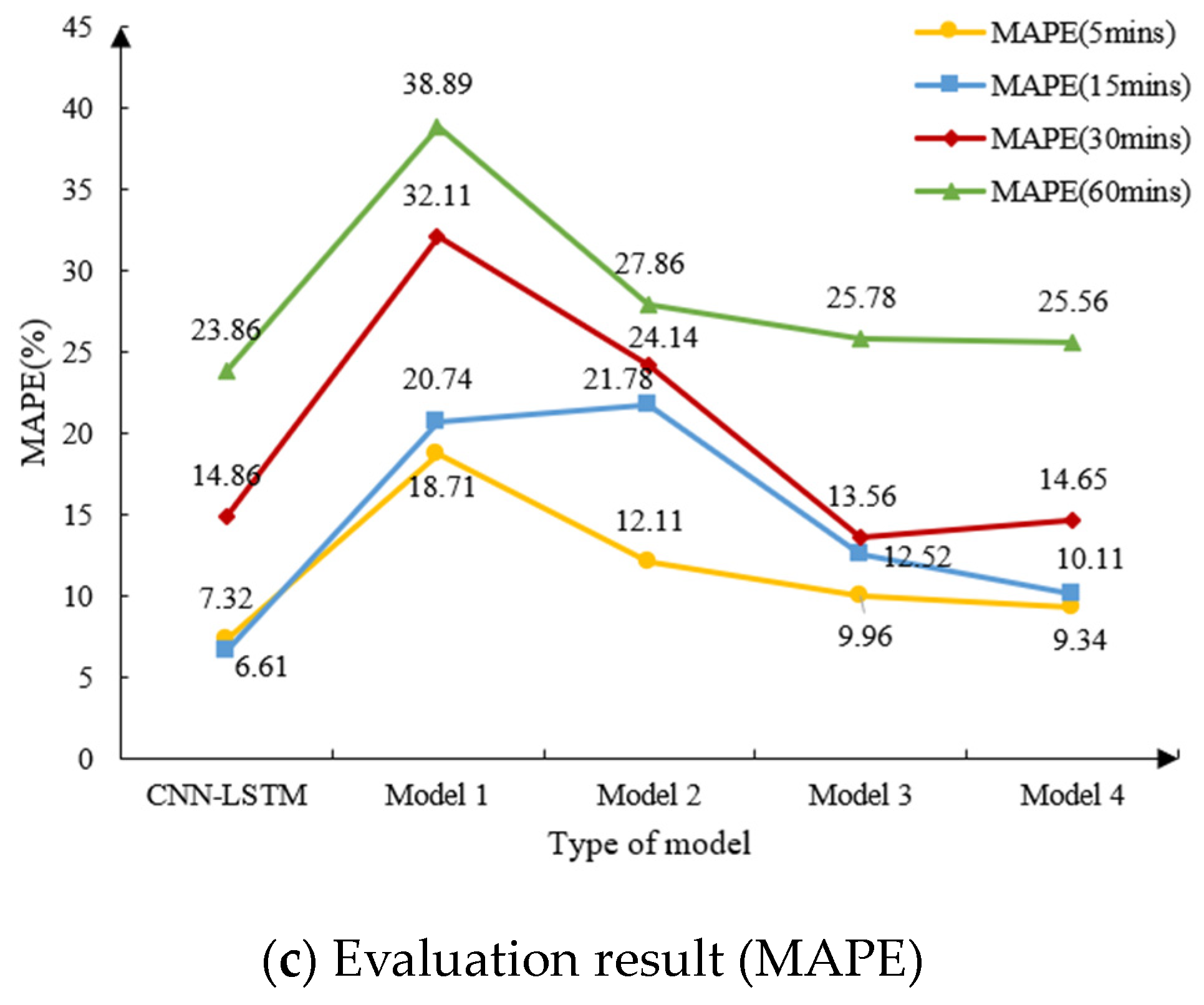
4.3.2. Evaluation of Traffic Flow Prediction Model

Based on the above contents, the reconstructed data are substituted into the CNN-LSTM fusion deep learning model proposed in this paper. In order to further illustrate the accuracy of the model, the overall model proposed in this paper is compared with an ARIMA model considering only time factors (referred to in this article as Model 1), an LSTM model considering only time factors (referred to in this article as Model 2), a CNN-LSTM model considering only time factors (referred to in this article as Model 3), and an LSTM model considering spatial–temporal correlation (referred to in this article as Model 4). The applicability of the model is measured with 5 min, 15 min, 30 min, and 1 h as time intervals. MAE, MSE, and MAPE are used as evaluation indexes to illustrate the accuracy of the proposed models. The final prediction results of CNN-LSTM are shown in Figure 9, and the comparative evaluation results of each model are shown in Figure 10.

It can be seen from Figure 9 that the fusion deep learning model considering spatial–temporal correlation proposed in this paper can well characterize the operation characteristics of traffic flow when the time interval is 5 min, 15 min, and 30 min. However, when the time interval is 60 min, due to the small amount of data in the training set, the model cannot accurately depict the rules of traffic flow, and the error of the test set is large.

As shown in Figure 10, the fusion deep learning model considering spatial–temporal correlation proposed in this paper has higher accuracy and applicability than Models 1, 2, 3, and 4. The high accuracy and applicability of the model are concentrated in the following four points:

(1) Model 1 is essentially a parametric regression method. Its inherent defect determines that it cannot accurately predict traffic flow time series of the target section. Therefore, the final accuracy is 81.29%, 79.26%, 67.89%, and 61.11% for different time intervals.

(2) Model 2 and Model 3 are essentially machine learning methods. As the number of iterations increases, the model can better learn the deep rules of traffic flow time series data, therefore it has higher accuracy than Model 1.

(3) Model 3 is a hybrid model, i.e., CNN can capture the dependence between sections of traffic flow forecasting problem, LSTM can capture the time dependence of traffic flow forecasting problem, and the established CNN-LSTM combination model can mine the rules and characteristics of data more deeply than Model 2. Therefore, compared with Model 2, its accuracy increases by 2.15%, 9.26%, 7.97%, and 2.08% at different time intervals. However, both Model 2 and Model 3 only consider the time series of traffic flow of the target section, while ignoring the impact of other sections highly correlated with the target section. Therefore, the forecast accuracy is lower than that of the proposed fusion deep learning model considering spatial–temporal correlation.

(4) Model 4 considers the spatial–temporal correlation of traffic flow data, but because it is not a mixed model in the same way as the previous point, the prediction accuracy is 2.01%, 3.50%, 0.02%, and 1.70% lower than the model proposed in this paper at different time intervals.

To sum up, compared with each evaluation index of the five models, the model proposed in this paper is optimal and has the smallest score for each error. When the interval of time series is 5 min, the values of MAE, MSE, and MAPE are 8.51, 15.71, and 7.32%; When the interval of time series is 15 min, the values of MAE, MSE, and MAPE are 13.41, 49.95, and 6.61%; When the interval of time series is 30 min, the values of MAE, MSE, and MAPE are 30.55, 60.68, and 14.86%; When the interval of time series is 60 min, the values of MAE, MSE, and MAPE are 45.08, 162.46 and 23.86%.The case study further proves the accuracy and applicability of the model in traffic flow prediction.

5. Conclusions

This paper proposes a fusion deep learning model considering spatial–temporal correlation to solve the problem of urban road traffic flow prediction and improve prediction accuracy. For the collected traffic flow monitoring data, in order to mine the spatial correlation between the target section and other sections, this paper establishes a road section similarity measurement method based on wavelet decomposition and dynamic time warping and verifies the accuracy and practicability of the method through empirical analysis. Then, the stability of the extracted traffic flow data of each section is analyzed to improve the overall accuracy of the model prediction. Finally, for the reconstructed traffic flow data, we extract spatial features through CNN, and then extract temporal features through LSTM, and train the fusion deep learning models to realize the traffic flow prediction.

This paper selects the traffic flow data of RTMS in Daxing District, Beijing, China for empirical verification. The empirical results show that the performance of the model in traffic flow prediction is better than the mainstream machine learning methods, and has excellent accuracy at the time intervals of 5 min, 15 min, and 30 min. However, the model still has room for improvement: For the traffic flow prediction at the time interval of 60 min, the accuracy of the model cannot be verified due to the lack of data. Moreover, the training cycle will be long when dealing with traffic flow data for large transportation networks. Therefore, we will consider training the traffic flow data with a larger time span and measuring the accuracy of the model at the time interval of 60 min. Moreover, in the future, we will optimize the structure of the fusion deep learning model to reduce errors in the traffic flow prediction tasks.

References

1. Gu, Y.; Lu, W.; Qin, L.; Li, M.; Shao, Z. Short-term prediction of lane-level traffic speeds: A fusion deep learning model. Transp. Res. Part C Emerg. Technol. 2019, 106, 1–16. [Google Scholar] [CrossRef]
2. Kumar, S.V.; Vanajakshi, L. Short-term traffic flow prediction using seasonal ARIMA model with limited input data. Eur. Transp. Res. Rev. 2015, 7, 21. [Google Scholar] [CrossRef] [Green Version]
3. Otoshi, T.; Ohsita, Y.; Murata, M.; Takahashi, Y.; Ishibashi, K.; Shiomoto, K. Traffic prediction for dynamic traffic engineering considering traffic variation. In Proceedings of the Global Communications Conference, Atlanta, GA, USA, 9–13 December 2013; IEEE: Piscataway, NJ, USA, 2014; pp. 1570–1576. [Google Scholar]
4. Boto-Giralda, D.; Dfaz-Pernas, F.J.; Gonzalez-Ortega, D.; Díez-Higuera, J.F.; Antón-Rodríguez, M.; Martínez-Zarzuela, M.; Torre-Díez, I. Wavelet-Based Denoising for Traffic Volume Time Series Forecasting with Self-Organizing Neural Networks. Comput.-Aided Civ. Infrastruct. Eng. 2010, 25, 530–545. [Google Scholar] [CrossRef]
5. Chan, K.Y.; Dillon, T.S.; Singh, J.; Chang, E. Neural-Network-Based Models for Short-Term Traffic Flow Forecasting Using a Hybrid Exponential Smoothing and Levenberg-Marquardt Model. IEEE Trans. Intell. Transp. Syst. 2012, 13, 644–654. [Google Scholar] [CrossRef]
6. Ch, S.; Anand, N.; Panigrahi, B.K.; Mathur, S. Streamflow forecasting by SVM with quantum behaved particle swarm optimization. Neurocomputing 2013, 101, 18–23. [Google Scholar] [CrossRef]
7. Yang, H.J.; Hu, X. Wavelet neural network with improved genetic model for traffic flow time series prediction. Optik 2016, 127, 8103–8110. [Google Scholar] [CrossRef]
8. Wang, K.; Ma, C.; Qiao, Y.; Lu, X.; Hao, W.; Dong, S. A hybrid deep learning model with 1DCNN-LSTM-Attention networks for short-term traffic flow prediction. Phys. A Stat. Mech. Its Appl. 2021, 583, 126293. [Google Scholar] [CrossRef]
9. Zhan, F.; Wan, X.; Cheng, Y.; Ran, B. Methods for multi-type sensor allocations along a freeway corridor. IEEE Intell. Transp. Syst. Mag. 2018, 10, 134–149. [Google Scholar] [CrossRef]
10. Yu, X.; Prevedouros, P.D. Performance and Challenges in Utilizing Non-Intrusive Sensors for Traffic Data Collection. Adv. Remote Sens. 2013, 2, 45–50. [Google Scholar] [CrossRef] [Green Version]
11. Wang, H.; Liu, L.; Dong, S.; Qian, Z.; Wei, H. A novel work zone short-term vehicle-type specific traffic speed prediction model through the hybrid EMD-ARIMA framework. Transp. B Transp. Dyn. 2015, 4, 159–186. [Google Scholar] [CrossRef]
12. Xie, H.H.; Dai, X.H.; Qi, Y. Improved K-nearest neighbor model for short-term traffic flow forecasting. J. Traffic Transp. Eng. 2014, 14, 87–94. [Google Scholar]
13. Dong, C.; Stephen, H.R.; Yang, Q.; Shao, C. Combining the statistical model and heuristic model to predict flow rate. J. Transp. Eng. 2014, 140, 06014001. [Google Scholar] [CrossRef]
14. Dong, C.; Shao, C.; Richards, S.H.; Han, L.D. Flow rate and time mean speed predictions for the urban freeway network using state space models. Transp. Res. Part C Emerg. Technol. 2014, 43, 20–32. [Google Scholar] [CrossRef]
15. Yang, L.H.; Zhang, C.; Qiu, X.Y.; Li, S.; Wang, H. Research progress on car-following models. J. Traffic Transp. Eng. 2019, 19, 125–138. [Google Scholar]
16. Zhan, X.; Li, R.; Ukkusuri, S.V. Link-based traffic state estimation and prediction for arterial networks using license-plate recognition data. Transp. Res. Part C Emerg. Technol. 2020, 117, 102660. [Google Scholar] [CrossRef]
17. Pan, Y.; Jin, X.; Li, Y.; Chen, D.; Zhou, J. A Study on the Prediction of Book Borrowing Based on ARIMA-SVR Model. Procedia Comput. Sci. 2021, 188, 93–102. [Google Scholar] [CrossRef]
18. Zhang, Z.; Li, M.; Lin, X.; Wang, Y.; He, F. Multistep speed prediction on traffic networks: A deep learning approach considering spatio-temporal dependencies. Transp. Res. Part C Emerg. Technol. 2019, 105, 297–322. [Google Scholar] [CrossRef]
19. Tian, Y.; Zhang, K.; Li, J.; Lin, X.; Yang, B. LSTM-based Traffic Flow Prediction with Missing Data. Neurocomputing 2018, 318, 297–305. [Google Scholar] [CrossRef]
20. Sun, X.; Munoz, L.; Horowitz, R. Mixture Kalman filter based highway congestion mode and vehicle density estimator and its application. In Proceedings of the American Control Conference, Boston, MA, USA, 30 June–2 July 2004; IEEE: Piscataway, NJ, USA, 2004; Volume 3, pp. 2098–2103. [Google Scholar]
21. Xu, D.W.; Wang, Y.D.; Jia, L.M.; Qin, Y.; Dong, H.H. Real-time road traffic state prediction based on ARIMA and Kalman filter. Front. Inf. Technol. Electron. Eng. 2017, 18, 287–302. [Google Scholar] [CrossRef]
22. Narmadha, S.; Vijayakumar, V. Spatio-Temporal vehicle traffic flow prediction using multivariate CNN and LSTM model. Mater. Today Proc. 2021, SSN, 2214–7853. [Google Scholar]
23. Do, L.N.; Vu, H.L.; Vo, B.Q.; Liu, Z.; Phung, D. An effective spatial-temporal attention based neural network for traffic flow prediction-ScienceDirect. Transp. Res. Part C Emerg. Technol. 2019, 108, 12–28. [Google Scholar] [CrossRef]
24. Wiseman, Y. Autonomous vehicles. In Encyclopedia of Information Science and Technology, 5th ed.; Bar-Ilan University: Ramat Gan, Israel, 2021. [Google Scholar]
Figure 1. The method flow of the proposed model.
Sustainability 13 10595 g001
Figure 2. Flow chart of traffic flow parameter feature extraction method.
Sustainability 13 10595 g002
Figure 3. LSTM model diagram.
Sustainability 13 10595 g003
Figure 4. Traffic detector distribution.
Sustainability 13 10595 g004
Figure 5. Data and processing results.
Sustainability 13 10595 g005
Figure 6. The one-week traffic flow trend of the target section.
Sustainability 13 10595 g006
Figure 7. Similarity measurement of time series.
Sustainability 13 10595 g007
Figure 8. Cross section traffic flow com parison.
Sustainability 13 10595 g008
Figure 9. Final prediction results of CNN-LSTM.
Sustainability 13 10595 g009
Figure 10. The comparative evaluation results of each model.
Sustainability 13 10595 g010aSustainability 13 10595 g010b